Oscillatory Waves in Discrete Scalar Conservation Laws
Abstract
We study Hamiltonian difference schemes for scalar conservation laws with monotone flux function and establish the existence of a three-parameter family of periodic travelling waves (wavetrains). The proof is based on an integral equation for the dual wave profile and employs constrained maximization as well as the invariance properties of a gradient flow. We also discuss the approximation of wavetrains and present some numerical results.
Keywords:
conservation laws, difference schemes, dispersive shocks,
travelling waves, Hamiltonian lattices, variational integrators
MSC (2000):
35L60, 37K60, 47J30
1 Introduction
This paper is concerned with oscillatory patterns in the nonlinear lattice equation
| (1) |
which is, up to an appropriate scaling, a centred difference scheme for the scalar conservation law
| (2) |
Although the lattice cannot be used for the approximate computation of (non-smooth) solutions of (2), there exist several reasons why it seems worth investigating the dynamical properties of (1) in greater detail. First, both the lattice and the PDE have the same Hamiltonian structure, and (1) can be regarded as a variational integrator for (2) with respect to the space discretization, see appendix A. Studying (1) therefore allows to understand in which aspects quasilinear Hamiltonian PDEs differ from their spatially discrete counterparts. Second, the lattice is, similar to Korteweg-de Vries-type (KdV) equations, a dispersive regularization of (2), and hence it generates dispersive shocks instead of Lax shocks. These dispersive shocks describe the fundamental mode of self-thermalization in dispersive Hamiltonian systems but are well understood only for systems that are completely integrable. The ODE system (1) provides a class of non-integrable examples which can be simulated effectively, for instance using variational integrators for the time discretization. Finally, discrete conservation laws provide toy models for more complicate Hamiltonian lattices. Fermi-Pasta-Ulam (FPU) chains, for instance, are equivalent to difference schemes for the so called -system, which is a nonlinear hyperbolic system of two conservation laws.
In what follows we focus on a particular aspect of the lattice dynamics and investigate special coherent structures, namely wavetrains. These are periodic travelling wave solutions to (1) and therefore linked to nonlinear advance-delay-differential equations.
We emphasize that all subsequent considerations require a centred difference operator in (1) as only this one gives rise to a Hamiltonian lattice. Other discrete scalar conservation laws, as for instance upwind schemes, have different dynamical properties and are excluded.
1.1 Dispersive shocks and wavetrains
The relation between (1) and (2) manifests under the hyperbolic scaling
| (3) |
where is the scaling parameter, and and denote the macroscopic time and particle index, respectively. On a formal level we can expand differences in powers of differential operators, i.e.,
so that, to leading order in , the lattice dynamics is governed by the KdV-type PDE
which is in fact a dispersive regularization of (2).

|

|

|

|

|

|

|

|

|
As already mentioned, a key feature of all dispersive regularizations of (2) are dispersive shocks.[17, 6, 5, 25] For illustration, and to motivate our analytical investigations, we now describe the formation of such dispersive shocks in numerical simulations of (1). For convenience we shall consider spatially periodic solutions with for some , which then defines the natural scaling parameter . Starting with long-wave-length initial data
where is a smooth and -periodic function in , we can solve (1) numerically by using the variational integrator (28). A typical example is depicted in Figure 2 for the data
| (4) |
For small macroscopic times , we observe that the data remain in the long-wave-length regime, so we can expect that the lattice solutions converge as in some strong sense to a smooth solution of (2). This convergence is not surprising in view of Strang’s theorem[29], see also the discussion in Ref. [11, 17]. At time , however, the solution to the PDE (2) forms a Lax shock, which then propagates with speed according to the Rankine-Hugoniot jump condition . After the onset of the shock singularity, the lattice solutions do not converge anymore to a solution of (2), not even in a weak sense, but exhibit strong microscopic oscillations. These oscillations spread out in space and time, and constitute the dispersive shock. This phenomenon is fascinating from both the mathematical and the physical point of view because the formation of dispersive shocks can be regarded as a self-thermalization of the nonlinear Hamiltonian system. We refer to Ref. [4, 16] for more details including a thermodynamic discussion of dispersive FPU shocks.
The observation that certain difference schemes for hyperbolic conservation laws produce dispersive shocks is not new, see for instance Ref. [22, 11], which investigate dispersive shocks in
This lattice also belongs to the class of equations considered here as it transforms via into (1) with , which is the completely integrable Kac-von Moerbeke lattice[20].
The key observation in our context is that the oscillations within a dispersive shock exhibit the typical behaviour of a modulated oscillation. As illustrated in Figure 2, the local oscillations in the vicinity of a given macroscopic point resemble a periodic profile function, and we can expect this profile to be generated by a single wavetrain. The parameters of this wavetrain, however, depend on and , which can be seen from the fact that each magnification in Figure 2 displays a another amplitude, wave number, and average.
The goal of this paper is to prove the existence of a three-parameter family of wavetrains for a huge class of nonlinear potentials . Since the only crucial assumption we have to make is strict convexity of , our results cover a large number of non-integrable variants of (1). Due to rigorous results for integrable systems, such as the KdV equation[23, 24] and the Toda chain[21, 2], we expect the parameter modulation within a dispersive shock to be governed by a variant of Whitham’s modulation equations.[30, 31] The formal derivation and investigation of this Whitham system, however, is left for future research. We also do not justify that the oscillations within dispersive shocks take in fact the form of modulated wavetrains. For a rigorous proof in non-integrable systems we still lack the analytical tools; a reliable numerical justification would be possible, and was carried out for FPU in Ref. [4], but is beyond the scope of this paper.
A travelling wave is a special solution to (1) with
| (5) |
where is the wave number, is the frequency, and the profile depends on the phase variable . In this paper we are solely interested in wavetrains, which have periodic , but mention that one might also study solitons and fronts having homoclinic and heteroclinic profiles, respectively.
Splitting into its constant and zero average part via , we infer from (1) that each wavetrain satisfies
| (6) |
where is defined by
1.2 Main result and organisation of the paper
Since the wavetrain equation (6) involves both advance and delay terms there is no notion of an initial value problem, and one has to use rather sophisticated methods to establish the existence of solutions. Possible candidates, which have proven to be powerful for other Hamiltonian lattices, are rigorous perturbation arguments[8], spatial dynamics with centre manifold reduction[18, 19], critical point techniques[28, 26, 27], and constrained optimization[9, 7, 14].
Our approach also exploits the underlying variational structure and restates (6) as
| (7) |
where is the dual profile to be introduced in §2.2. Moreover, is a compact and symmetric integral operator, and is the dual potential, i.e., the Legendre transform of . This formulation allows to construct wavetrains as solutions to a constrained optimization problem, where and play the role of Lagrangian multipliers.
The existence proof for wavetrains given below is based on a combination of variational arguments (direct method) and dynamical concepts (invariant sets of flows). These ideas can also be applied to other Hamiltonian lattices and different types of coherent structures[12, 15, 13], but discrete scalar conservation laws are special since they are first order in time and real-valued. All other Hamiltonian lattices we are aware of are either second order in time or vector-valued, and allow for a simpler variational setting for travelling waves.
Our main result guarantees the existence of a three-parameter family of wavetrains and can be summarized as follows.
Main result. Suppose that is strictly convex and satisfies some regularity assumptions. Then, for each there exists a two-parameter family of -periodic wavetrains with and frequency such that the profile is even and unimodal on .

|

|

|
The assumptions on will be specified in Assumption 2 and the precise existence result is formulated in Theorem 8. Here we proceed with some comments concerning the choice of and the convexity of .
- 1.
- 2.
As time reversal in (1) corresponds to , the existence result can easily be adapted to the case of strictly concave .
- 3.
Our proof does not cover potentials that change from convex to concave or vice versa, and it is not obvious what happens near zeros of . Numerical simulations as presented in Figure 3, however, indicate that then a three-parameter families of wavetrains might not exist anymore.
The paper is organized as follows. In §2 we summarize some elementary properties of wavetrains. We also derive the integral equation for the dual profile and discuss some normalization which allows to simplify the presentation. §3 is devoted to the proof of the existence result. To point out the key idea we first state an abstract result in Theorem 3, and show afterwards that the assertions we made are satisfied for wavetrains, see Theorem 8. Finally, in §4 we compute wavetrains by means of a discrete gradient flow on a constraint manifold.
2 Preliminaries about discrete conservation laws
In this section we summarize some elementary properties of wavetrains, derive the integral equation (7) for the dual profile, and introduce some normalization.
2.1 Elementary properties and special solutions
First we observe that the wavetrain equation (6) is invariant under shifts , reflections , and scalings
with . It is therefore sufficient to consider a fixed periodicity cell and wave numbers , so from now on we assume
Recall that a periodic function is even if holds for all , and that an even function on is unimodal if it is monotone on .
Second, we notice that (6) degenerates for both and . In fact, wavetrains for are globally constant with , while wavetrains for are stationary binary oscillations with and . Therefore, and since (6) is invariant under , we restrict all subsequent considerations to .

|

|

|

|

|

|
For linear flux we can solve (6) by Fourier transform. Specifically, linearizing (6) around and restricting to unimodal and even profiles we find that depends on and via the dispersion relation
and that the unique profile is , where the amplitude is the third independent parameter. Harmonic wavetrains furthermore exemplify that simple profiles can generate rather complex patterns for the spatial oscillations in the lattice. This is illustrated in Figure 4, and in Figure 9 for the nonlinear case.
The second case in which we can solve (6) explicitly are wavetrains with wave number .
Lemma 1.
Each wavetrain for satisfies the Hamiltonian ODE
| (8) |
where
In particular, if is smooth and convex, then for each there exists a unique one-parameter family of wavetrains with unimodal and even profiles that is parametrized by .
2.2 Integral equation for the dual profile and normalization
We define the dual profile of a wavetrain by
| (9) |
where abbreviates the integral mean value, i.e.,
The key ingredient to our variational existence proof is to restate (6) as an equation for . To this end we consider the Legendre transform of , which is well-defined and strictly convex provided that is strictly convex[3], and satisfies
Using and (9) we now find that (6) is equivalent to
and integration with respect to yields
| (10) |
Here, appears as a constant of integration and the integral operator is defined by
| (11) |
With (10) we have derived the dual formulation of (6); the main mathematical difference between both formulations will be discussed at the end of §3.1.
For the existence proof in §3 it is convenient to normalize (10) in two steps. At first we incorporate the parameter into the nonlinearity by considering the normalized dual potential
| (12) |
which satisfies
This transforms (10) into
The second normalization step is motivated by the harmonic case and the observation that the formula for the phase speed depends on the value of . In fact, the linearization of (10) around gives the dispersion relation
and we conclude that for but for , see Figure 5. We also notice that has slightly different properties for and . In particular, by (11) we have
| (13) |
for all with , where denotes the shift operator

To complete the normalization we now replace by , and by either or , which are defined for by
Specifically, for we restate the dual wavetrain equation (10) as
| (14) |
whereas for we write
| (15) |
Notice that for both formulations agree and encode the ODE solution from Lemma 1. In particular, in this case we have the further symmetry .
3 Variational existence proof for wavetrains
In this section we prove the existence of a three-parameter family of wavetrains by showing that the dual integral equations (14) and (15) possess corresponding three-parameter families of solutions. To elucidate the key ideas we start with an abstract existence result in §3.1, and check the validity of its assumptions in §3.2.
From now on we rely on the following standing assumption.
Assumption 2.
is twice continuously differentiable and strictly convex with
for all and some constants , .
We remark that Assumption (2) holds if and only if , the Legendre transform of , is twice continuously differentiable and strictly convex with . This follows from basic properties of the Legendre transform[3].
Throughout the remainder of this paper, denotes the usual Hilbert space of square-integrable and periodic functions on the periodicity cell , where the dual pairing and the integral norm are normalized via
Moreover, we define
3.1 Variational approach and abstract existence result
We now prove the existence of a one-parameter family of solutions to the abstract wavetrain equation (7). To this end we assume that the operator is compact and symmetric, and that is normalized by
| (16) |
Our variational approach to (7) is based on the functionals
| (17) |
and the constrained optimization problem
| (18) |
where is a free parameter. We readily justify that (7) is the corresponding Euler-Lagrange equation for a maximizer , where and are Lagrangian multiplies for the constraints and , respectively.
The existence of maximizers can be proven by the direct method using weak compactness arguments, see the first part in the proof of Theorem 3. However, in order to gain more qualitative information about shape of the profile function we refine the optimization problem (18). For this purpose we introduce the corresponding (negative) gradient flow, that is the -valued ODE
| (19) |
Here is the flow time, and
are two dynamical multipliers which guarantee that and hold along each trajectory of (19). Notice that, by construction, each stationary point of (19) solves (7) with and , and vice versa. For later use we also mention that the explicit Euler scheme to (19) with time step is given by the mapping
| (20) |
We are now able to formulate the refined existence result.
Theorem 3.
In preparation for the proof of Theorem 3 we draw the following conclusions from Assumption 2, the normalization condition (16), and the postulated properties of .
Lemma 4.
The following assertions are satisfied.
- 1.
is well defined and weakly continuous,
- 2.
is well defined, convex, continuous, and Gâteaux-differentiable with derivative . We also have
(21) for all .
- 3.
For each , the set is convex and weakly compact in . It is also star-shaped in the sense that for each there exists a unique such that for all .
Lemma 5.
The gradient flow (19) is well defined on and conserves . Moreover, increases strictly on each non-stationary trajectory.
Proof.
Suppose that is given with , that means . The strict convexity of implies and gives . From this we infer that is well defined for . Consequently, and since the right hand side in (19) is locally Lipschitz in , the ODE (19) is well posed in . By straight forward computations we now verify and
In particular, we have if and only if and are collinear, i.e., if and only if is a stationary point of (19). ∎
We now finish the proof of the abstract existence result.
Proof of Theorem 3.
With respect to the weak topology in , the objective functional is continuous and the constraint set is compact. The existence of a maximizer thus follows from basic topological principles, and by assumption we have . By Lemma 4 we find
which implies . On the other hand, yields , and thus we find , which means . Moreover, Lemma 5 ensures that is stationary under the gradient flow (19), and hence a solution to (7). Finally, testing (7) with we find
and combined with (21) implies . ∎
To conclude this section we mention that there also exist variational characterizations of solutions to (6), but these are less feasible than the integral equation for the dual profile. The analogue to (7) is
which has a variational structure, but a direct treatment is difficult as is not continuous. One can get rid off by making the ansatz with and working with the functionals
However, the level sets of neither nor are weakly compact, and therefore it is not obvious how to set up a variational framework that allows to prove the existence of solutions. Finally, one might think about solving the equation by fixed point arguments, but then one has find a way to exclude the trivial solution .
3.2 Proof of the main result
Here we apply the abstract result from the previous section and prove the existence of a three-parameter family of wavetrains as claimed in the introduction. We therefore define to be the positive cone of all -functions on that are even, unimodal, and have zero average. This reads
| (22) |
We next summarize some properties of the averaging operator .
Lemma 6.
For all the operator maps into itself and is symmetric and compact. Moreover, it maps into .
Proof.
The first three assertions follow directly from (11). It remains to prove that is invariant under for ; the claim for then follows from (13) and the fact that . Let be given, and notice that is even with weak derivative . For , the periodicity and the evenness of imply where , so the monotonicity of in gives . Similarly, for and we have and , respectively. In summary, is increasing on , and since it is also even, the proof is complete. ∎
Lemma 6 guarantees that both and are symmetric and compact, and map and .
Lemma 7.
Proof.
The cone is convex and closed, and we have with Therefore, it remains to show that is invariant under the gradient flow (19). To this end we remark that is invariant under the action of the operator if and only if the function is non-decreasing. We now consider the Euler scheme of the gradient flow (20) with time step , that is
where the family of nonlinear functions is given by
Thanks to Assumption 2, for each bounded set there exists such that holds true for all , all , and all . From this, the invariance of under the action of , and the continuous dependence of and on , we conclude that for each ball there exists such that maps into for all . The claimed invariance of the gradient flow now follows by passing to the limit . ∎
We are now able to concretize the informal existence result from the introduction as follows.
Theorem 8.
Let , , and be given. Then, there exist profiles along with multipliers and , such that
In particular, the profile solves
with and , whereas solves
with and .
Proof.
We conclude this section with some remarks concerning the assumptions and assertions of Theorems 3 and 8.
- 1.
The strict convexity of (or equivalently, of ) is crucial for our existence proof. In fact, it is truly necessary for relating the integral equations (14) and (15) to the wavetrain equation (6). It also plays an important role in the proof of Theorem 3 as it guarantees the weak compactness of . The assumptions about upper and lower bounds for , however, are made for convenience and might be weakened for the price of more technical effort.
- 2.
It would be highly desirable to give uniqueness results that classify wavetrains up to phase shifts and scalings of the periodic cell. In analogy to the harmonic case, we conjecture that the three-parameter family from Theorem(8) contains all wavetrains which satisfy the profile constraint , but we are not able to prove this. Another open problem is the stability of wavetrains.
- 3.
Obviously, in Theorem 3 we can choose to obtain solutions to the original optimization problem (18). In this case, (7) is provided by the Lagrangian multiplier rule. If , however, is a proper subset of then the validity of (7) does not follow from the multiplier rule but is a consequence of the invariance properties of . We also remark that numerical simulations indicate that each maximizer of in is (up to phase shifts) unimodal and even, and hence contained in . We therefore conjecture that (18) and its refined variant from Theorem 3 have the same solutions, but a rigorous proof is not available.
4 Numerical simulations
In this section we illustrate our analytical findings by numerical simulations, which are computed by the following implementation of the discrete gradient flow (20) with instead of , see (12), and and for and , respectively:

|

|

|

|

|

|


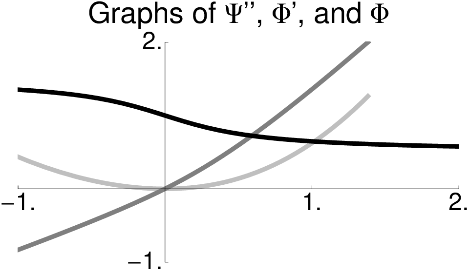


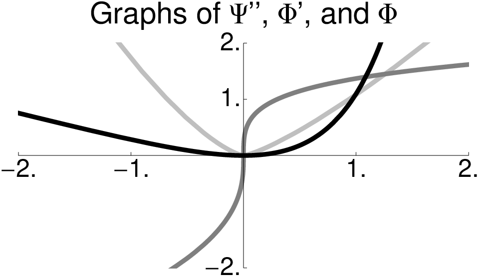
| Example (23) | Example (24) | Example (25) |
|---|---|---|

|

|

|

|

|

|

|

|

|

|

|

|

|

|

|
- 1.
We sample the periodicity cell by grid points with .
- 2.
We approximate by and replace all integrals with respect to by Riemann sums.
- 3.
After each update step according to (20), we enforce the conservation of by a scaling , where the factor is computed by a single Newton step.
- 4.
For given and , we initialize the scheme with , where the amplitude determines via .
Although this numerical scheme is rather simple it shows good convergence properties, provided that is sufficiently large and the time step is sufficiently small. All simulation presented below are performed with and .
The first example concerns the data
| (23) |
where is determined by as described above. The numerical results are presented in Figure 6, which shows the dual profile as function of for several values of . We also refer to Figure 9, which illustrates how the wavetrains appear in snapshots against . A special feature of this example is that is even for , and this implies that (7) is invariant under . We therefore find that the profiles are the same for and , and exhibit the further symmetry .
The second example is computed with
| (24) |
and illustrates the generic case that is not even. In Figure 8 we therefore observe that the profiles do not satisfy anymore, and are no longer the same for and .
Appendix A Lagrangian and Hamiltonian structures for scalar conservation laws
For the readers convenience we summarize some basic fact about the Lagrangian and Hamiltonian structures of discrete scalar conservation laws. Both structures are very similar to the respective structures for the KdV equation, compare for instance [1], and originate from the skew-symmetry of centred difference operators. Specifically, for with the identity
holds for all sequences for which the series are well-defined. Notice that the one-sided difference operators with are not skew-symmetric but satisfy .
To derive the Lagrangian structure we assume that there exists such that . This transform (1) into
| (26) |
and reveals that the action integral is given by
| (27) |
where is a given final time. In fact, computing the variational derivatives and we easily check that (26) is just the Euler-Lagrange equation .
A special feature of is that the canonical momenta do not depend on , and therefore we cannot apply the standard procedure to derive the Hamiltonian structure. There is, however, a non-canonical Hamiltonian structure. Using the Hamiltonian
the discrete scalar conservation law (1) can be written as
This is indeed a Hamiltonian equation, where acts as non-canonical symplectic operator that corresponds to the symplectic product
The PDE (2) has the same Lagrangian and Hamiltonian structures in the sense that all formulas from above remain valid provided that we apply the scaling (3), replace sums over by integrals with respect to , and employ the differential operator instead of . In other words, the scalar conservation law (2) is the Euler-Lagrange equation to the action integral
It is moreover equivalent to
which has Hamiltonian and symplectic product . The analogies between the structures of lattice and PDE are – in view of the skew-symmetry of both and – not surprising and exemplify the more general principles laid out in [10]. Moreover, if we replace by the macroscopic difference operator
we easily recover the scaled version of (1). In this sense the lattice (1) is just a variational integrator of the scalar conservation law (2), i.e., a semi-discrete scheme that respects the underlying variational and symplectic structures.
The very same idea also allows to derive variational integrators for the time discretization. If we replace the continuous time derivative in (27) by , where is the time step size and the index refers to the time step, we obtain the discrete action integral
which depends on all the ’s. Evaluating the Euler-Lagrange equation , and replacing by , yields the fully discrete scheme
| (28) |
which also served to compute the numerical examples from §1.
Acknowledgements
This work was supported by the EPSRC Science and Innovation award to the Oxford Centre for Nonlinear PDE (EP/E035027/1).
References
- [1] R. Abraham and J.E. Marsden, Foundations of Mechanics, 2. ed., Perseus books, Cambridge Massachusetts, 1978, Updated 1985 Printing.
- [2] P. Deift and T.-R. McLaughlin, A continuum limit of the Toda lattice, Mem. Americ. Math. Soc., vol. 131/624, American Mathematical Society, 1998.
- [3] E. DiBenedetto, Real Analysis, Birkhäuser Advanced Texts: Basler Lehrbücher, Birkhäuser Boston, 2002.
- [4] W. Dreyer and M. Herrmann, Numerical experiments on the modulation theory for the nonlinear atomic chain, Physica D 237 (2008), no. 2, 255–282.
- [5] W. Dreyer, M. Herrmann, and J. Rademacher, Pulses, traveling waves and modulational theory in oscillator chains, Analysis, Modeling and Simulation of Multiscale Problems (A. Mielke, ed.), Springer, 2006.
- [6] G.A. El, Resolution of a shock in hyperbolic systems modified by weak dispersion, Chaos 15 (2005), 037103.
- [7] A.-M. Filip and S. Venakides, Existence and modulation of traveling waves in particle chains, Comm. Pure Appl. Math. 51 (1999), no. 6, 693–735.
- [8] G. Friesecke and R.L. Pego, Solitary waves on FPU lattices. I. Qualitative properties, renormalization and continuum limit, Nonlinearity 12 (1999), no. 6, 1601–1627.
- [9] G. Friesecke and J.A.D. Wattis, Existence theorem for solitary waves on lattices, Comm. Math. Phys. 161 (1994), no. 2, 391–418.
- [10] J. Giannoulis, M. Herrmann, and A. Mielke, Lagrangian and Hamiltonian two-scale reduction, J. Math. Phys. 49 (2008), no. 10, 103505, 42.
- [11] J. Goodman and P. Lax, On dispersive difference schemes, Comm. Pure. Appl. Math. 41 (1988), 591–613.
- [12] M. Herrmann, Periodic travelling waves in convex Klein-Gordon chains, Nonlinear Anal.-Theory Methods Appl. 71 (2009), no. 11, 5501–5508.
- [13] , Heteroclinic standing waves in defocussing DNLS equations, to appear in Applicable Analysis, 2010.
- [14] , Unimodal wavetrains and solitons in convex Fermi-Pasta-Ulam chains, Proc. R. Soc. Edinb. Sect. A-Math. 140 (2010), no. 04, 753–785.
- [15] M. Herrmann and J. D. M. Rademacher, Heteroclinic travelling waves in convex FPU-type chains, SIAM J. Math. Anal. 42 (2010), no. 4, 1483–1504.
- [16] , Riemann solvers and undercompressive shocks of convex FPU chains, Nonlinearity 23 (2010), no. 2, 277–304.
- [17] T.Y. Hou and P. Lax, Dispersive approximations in fluid dynamics, Comm. Pure Appl. Math. 44 (1991), 1–40.
- [18] G. Iooss, Travelling waves in the Fermi-Pasta-Ulam lattice, Nonlinearity 13 (2000), 849–866.
- [19] G. Iooss and G. James, Localized waves in nonlinear oscillator chains, Chaos 15 (2005), 015113.
- [20] M. Kac and P. van Moerbeke, On an explicitly soluble system of nonlinear differential equations related to certain Toda lattices, Advances in Math. 16 (1975), 160–169.
- [21] S. Kamvissis, On the long time behavior of the double infinite toda chain under shock initial data, Ph.D. thesis, New York University, 1991.
- [22] P.D. Lax, On dispersive difference schemes, Physica D 18 (1986), 250–254.
- [23] P.D. Lax and C.D. Levermore, The small dispersion limit of the Korteweg-de Vries equation, I, II, III, Comm. Pure Appl. Math. 36 (1983), no.3, 253–290; no.5, 571–593; no.6, 809–830.
- [24] P.D. Lax, C.D. Levermore, and S. Venakides, The generation and propagation of oscillations in dispersive initial value problems and their limiting behavior, Important developments in soliton theory (A.S. Fokas and V.E. Zakharov, eds.), Springer, 1993, pp. 205–241.
- [25] P.D. Miller and Zh. Xu, On the zero-dispersion limit of the Benjamin-Ono Cauchy problem for positive initial data, preprint, see arXiv:1002.3278, 2010.
- [26] A. Pankov and K. Pflüger, Traveling Waves in Lattice Dynamical Systems, Math. Meth. Appl. Sci. 23 (2000), 1223–1235.
- [27] H. Schwetlick and J. Zimmer, Solitary waves for nonconvex FPU lattices, J. Nonlinear Sci. 17 (2007), no. 1, 1–12.
- [28] D. Smets and M. Willem, Solitary waves with prescribed speed on infinite lattices, J. Funct. Anal. 149 (1997), 266–275.
- [29] G. Strang, Accurate partial difference methods. II. Non-linear problems, Numer. Math. 6 (1964), 37–46.
- [30] G.B. Whitham, Non-linear dispersive waves, Proc. Roy. Soc. Ser. A 283 (1965), 238–261.
- [31] , Linear and Nonlinear Waves, Pure And Applied Mathematics, vol. 1237, Wiley Interscience, New York, 1974.