Casimir Energies of Cylinders: Universal Function
Abstract
New exact results are given for the interior Casimir energies of infinitely long waveguides of triangular cross section (equilateral, hemiequilateral, and isosceles right triangles). Results for cylinders of rectangular cross section are rederived. In particular, results are obtained for interior modes belonging to Dirichlet and Neumann boundary conditions (TM and TE modes). These results are expressed in rapidly convergent series using the Chowla-Selberg formula, and in fact may be given in closed form, except for general rectangles. The energies are finite because only the first three heat-kernel coefficients can be nonzero for the case of polygonal boundaries. What appears to be a universal behavior of the Casimir energy as a function of the shape of the regular or quasi-regular cross-sectional figure is presented. Furthermore, numerical calculations for arbitrary right triangular cross sections suggest that the universal behavior may be extended to waveguides of general polygonal cross sections. The new exact and numerical results are compared with the proximity force approximation (PFA).
pacs
03.70.+k,11.10.Gh,42.50.Lc,42.50.PqI Introduction
Casimir’s seminal 1948 paper [1], demonstrating that two perfectly conducting parallel plates placed in vacuum attract, created something of a stir in the physics community because of its unexpected nature. In principle, it was verified experimentally in 1958 by Sparnaay [2], although conclusive measurements had to wait until the end of the 20th century [3, 4, 5]. Even more sensational was Boyer’s 1969 [6] calculation for the Casimir energy of a perfectly conducting spherical shell, which produced a repulsive force, rather than the attractive force that Casimir had postulated earlier [7] for a model of the electron. Since then, the question of how the sign and magnitude of the Casimir energy depend on the geometry of the system has been a constant leitmotif in Casimir energy studies.
In this paper, we attempt to elucidate this question by calculating the Casimir energies for the interiors of infinitely long cylinders of various cross sections. Such calculations have long been available for waveguides of rectangular [8, 9] and circular [10, 11] cross sections, but it apparently was not widely appreciated that energies for certain triangular cross sections were equally well calculable. We will work with triangular (equilateral, hemiequilateral, and isosceles right triangles), square, and rectangular cross sections. The triangular and rectangular cylinders are ideal since their eigenvalues are known explicitly. We obtain results in a very efficient form extremely amenable to numerical evaluation by use of the Chowla-Selberg formula [12, 13, 14], which is far more rapidly convergent than the direct evaluation of Epstein zeta functions. Even better, we are able to obtain closed-form results for the interior Casimir energies by use of a convenient representation found by many authors [15, 16, 17, 18, 19, 20, 21, 22]. These powerful methods supersede the previous method of directly summing the Epstein zeta function. With the obtained data, we can then relate Casimir energies for these cross sections with their distinguishing geometrical properties, notably the perimeter and the cross-sectional area . Our chief result is the discovery that there appears to be universal functional dependence for the Casimir energy per length multiplied by the area, , due to the interior fluctuations inside an infinitely long waveguide, in terms of a dimensionless quantity expressing the waveguide’s cross-sectional attributes, . This universality class applies to figures based on regular polygons; for a rectangle, for example, of sides and a different dependence obtains, which changes sign, as expected, when the rectangle becomes sufficiently elongated.
It is interesting to note that the square and circular waveguides have been extensively studied [8, 9, 23, 24, 25, 26, 10, 11, 27], in contrast to the triangular case which has only partially been examined. As far as the authors can tell, this paper is the first with explicit numerical results for the interior Casimir energy for infinitely long waveguides of triangular cross sections. Earlier work has, however, been done on plane equilateral triangular geometries [28]. For other work on equilateral triangular domains see Refs. [20, 21, 22, 29, 30]. There has been recent work in which explicit eigenvalues for the equilateral triangle have been used in computing numerical values for a piston of such a cross section [31].
Probably the reason why these Casimir energies were never evaluated, although the explicit eigenvalues appear in textbooks [33, 32], is that most authors considered interior calculations suspect. It is, of course, not possible by these methods to extract exterior eigenvalues or the corresponding Casimir energies. For smooth surfaces, such as a circular cylinder, only the sum of the interior and exterior Casimir energies of an infinitesimally thin boundary shell can be calculated unambiguously. In the language of heat kernels, the heat kernel coefficient is proportional to the cube of the curvature, and cancels only when both interior and exterior modes are included. When and only the interior is considered, there is a logarithmic divergence that cannot be removed, leaving an ambiguous Casimir energy. But, for polygonal boundaries, there is no such coefficient, and the interior Casimir energies seem well defined. There are divergences associated with the corners, but they do not contribute to the global Casimir energy of the waveguide, because they may be unambiguously subtracted off. For a review of the state of the art for self-energies of smoothly bounded regions, see Ref. [34]
The outline of this paper is as follows. In Sec. II we formulate Casimir energies in terms of mode summations, which we regulate either by dimensional continuation or by a temporal point-splitting cutoff. The former approach leads naturally to the use of the Chowla-Selberg formula, while the latter produces an expression that is summed through use of the Poisson summation formula; either approach can lead to a result that can, in special cases, be expressed in closed form. These machineries are applied to cylinders with equilateral triangular cross sections in Sec. III, for both Dirichlet and Neumann scalar modes, and hence for interior electromagnetic modes for a perfectly conducting boundary. The same is done in Sec. IV for a bisected equilateral triangular cross section, that is, a hemiequilateral or 30∘-60∘-90∘ triangle. A square cylinder is reconsidered in Sec. V, as is a rectangular cylinder in Sec. VI. The bisection of a square waveguide, one formed by a right isosceles triangle, is treated in Sec. VII. General right triangular cross sections are considered numerically in Sec. VIII, showing that a finite Casimir energy is obtained even when the eigenvalues are not explicitly available. All the energies for triangular Dirichlet boundaries found in this paper lie on a universal curve, which smoothly joins the proximity force approximation. Why the interior modes of a continuous curved cross section, such as that of a circle, cannot yield a finite Casimir energy is discussed in Sec. IX. The corner divergences are reflected only in the heat-kernel coefficient, unlike the curvature divergences which show up also in the coefficient. Again, unlike for continuously curved figures in a plane, Casimir energies for squares and equilateral triangles, and figures obtained from these by bisection, are likewise unambiguously calculable, and given in Sec. X, along with numerical results for right triangles. Results for the cylindrical geometries considered are summarized in the Conclusions in Sec. XI. The Appendix sketches the derivation of the Chowla-Selberg summation formula from the Abel-Plana formula.
II Casimir Energy of a Cylinder
II.1 Mode summation
The Casimir energy per length, , for infinite cylindrical geometries can generally be expressed as a sum over mode frequencies in the following form,
| (1) |
where are the eigenvalues of the two-dimensional Laplacian, , subject to satisfying appropriate boundary conditions on the cylinder’s surface. Here, denotes the two coordinates transverse to the longitudinal cylinder axis. For cases where the eigenvalues have explicit formulas, is a quadratic function of the mode numbers and .
The form of this quadratic function depends on the geometry, and the range of the mode numbers depends on the boundary conditions being applied. In the subsequent sections, we will look at the cases of Dirichlet and Neumann boundary conditions. The electromagnetic case can be obtained from these two classes of modes. Because of the cylindrical geometry, the modes of the electromagnetic field in a perfectly conducting waveguide can be expressed in terms of two scalar fields satisfying separately Dirichlet (E or TM modes) and Neumann boundary conditions (H or TE modes) [33, 32]. It follows then that the Casimir energy for an electromagnetic field is simply the sum of the Casimir energies for the E and H modes. (This breaks down if the boundaries are imperfect, for example, for a general dielectric cylinder [35].)
The expression above for the energy is formally divergent and as usual requires a regularization technique in order to obtain physically interpretable results. Out of the many ways to regularize such an expression, we choose the methods of dimensional regularization and point-splitting regularization.
II.2 Regularization methods
II.2.1 Dimensional regularization
By extending the one dimension for the longitudinal wavevector to dimensions, , we obtain the following expression for the energy per length,
| (2) |
In the limit , we obtain a divergence. However, one can surmount this problem by analytic continuation. For the cases considered in this paper, the eigenvalue expression is a simple quadratic form in and . This allows us to employ the Chowla-Selberg formula, an exact formula for a class of Epstein zeta functions [12, 13], proved in the Appendix, and thereby utilize the reflection property of the zeta function,
| (3) |
which allows us to continue to . The technique of dimensional regularization is our method of choice throughout this paper since the Chowla-Selberg formula converges exponentially faster than the Epstein zeta functions obtained by the point-splitting regularization we present below.
II.2.2 Point-splitting regularization (Cutoff)
A more physical approach is to start from the general form for the quantum vacuum energy in terms of the Green’s function for a given frequency ,
| (4) |
which for the situation of a cylindrical waveguide, gives the energy per length
| (5) |
where in the second line we have made a Euclidean rotation, , as well as introduced a time-splitting regulator, , where we are to take to zero at the end of the calculation. Assuming , we do the integration by closing it in the upper half plane, with the result
| (6) | |||||
Just as the dimensional regularization method was paired with the analytic continuation of the exponent, followed by use of the Chowla-Selberg formula, the cutoff regularization method is combined with Poisson’s sum formula. After rearranging the summations to span to , the summation is converted by Fourier transformation from one involving powers of to powers of . The final expression after simplifications is similar to the Chowla-Selberg result except for a slowly converging double sum. As noted above, in fact, that double sum can in special cases be summed into an explicit closed form; both regularizations give the same answer and thus serve as somewhat independent consistency checks. In addition, the cutoff regularization, unlike the dimensional-zeta-function regularization, exhibits the explicit divergences. We are then able to identify a “volume” and a “surface” divergence, as well as a divergent term independent of the scale of the cross section. All of these divergent terms can be regarded as contact terms, and, therefore, may be discarded. Corner divergences occur only in the constant term.
III Equilateral Cylinder

We consider an infinitely long cylinder of equilateral triangular cross section with side length and height , as shown in Fig. 1. The eigenvalues of the Laplacian on an equilateral triangular surface with Dirichlet or Neumann boundary conditions (solved by G. Lamé [36]) are of the form , where [33, 32]. Using this constraint, the previous expression can be simplified resulting in
| (7) |
Here, and are positive or negative integers; their allowed values depend on the boundary conditions, as indicated below. The eigenfunctions (which are given in Refs. [33, 32]) have degeneracy under cyclic or anticylic permutations of the three indices , , , so a factor of must be inserted before the mode sum. One would, indeed, expect only two mode numbers as it is a two-dimensional surface; however, the earlier form is more useful for counting degeneracies.
III.1 Dirichlet boundary
Dirichlet boundary conditions require the fields to vanish on the boundary , . The mode numbers are now restricted to , , and . If any index vanishes, the corresponding eigenfunction would likewise vanish. One can then use Eq. (1) with Eq. (7), and perform the appropriate sum over and to obtain the Casimir energy. The dimensionally regulated expression (2) may be evaluated by using the Chowla-Selberg formula, for :
| (8) |
However, it is valid only when the discriminant . The double prime indicates is excluded from the summation range. The divisor function, , is the sum of the -th powers of the divisors of ,
| (9) |
In the particular case of the Dirichlet equilateral triangle, . The special mode sum to be evaluated involves the explicit exclusion of the case when one of the mode labels vanishes:
| (10) | |||||
After a few manipulations such as use of the reflection property (3) we obtain
The above expression converges very fast and reaches an accuracy of twenty decimal places when just the first eight terms in the sum are included,
| (12) |
III.2 Neumann boundary
For Neumann boundary conditions, the normal derivative of the eigenfunctions must vanish on the boundary, . The restriction on the mode numbers is less severe than the Dirichlet case: here one of the mode numbers can be zero, but not two simultaneously. This gives a different summation range from that for the Dirichlet case, and after similar regularization manipulations, we obtain the result
| (13a) | |||||
| (13b) | |||||
III.3 EM perfectly conducting boundary
As discussed in the Introduction, the electromagnetic Casimir energy in the interior of perfectly conducting waveguide having an equilateral triangular cross section is simply the sum of the two previous energies,
| (14a) | |||||
| (14b) | |||||
| Note that while the Dirichlet energy is positive, the electromagnetic energy is negative, because the H mode overwhelms the E mode. | |||||
III.4 Point-splitting regularization
Poisson’s summation formula gives an expression equivalent to the original sum in terms of the summand’s Fourier transform:
| (15) |
This is useful for converting formulas most readily applicable for a large parameter to one most convenient when the parameter is small—that is, it is a duality transformation.
We will demonstrate this regularization method with the Dirichlet equilateral triangle. The mode sum in the energy (6) can be given explicit form as
| (16) |
where is given by Eq. (7), and the sums on the right hand side extend over all integer values, positive, negative, and zero. We first perform a transformation on with and . It follows that
| (17) | |||||
where now , and the and sums again extend over all integers. In a manner similar to Ref. [8], we adopt spherical coordinates and evaluate the generic Fourier transforms:
| (18) | |||||
where we have defined the vectors and . Carrying out the radial and angular integrals, we find straightforwardly
| (19b) | |||||
| (19c) | |||||
in terms of the abbreviation . With the appropriate coefficients for the Dirichlet equilateral triangle case, we isolate the divergences in the energy:
| (20) |
We note that the “volume” and “surface” divergent terms, which are respectively proportional to the area of the triangle and the perimeter , are as expected, and are presumably not of physical relevance. The last term, a constant in , certainly does not contribute to the self-stress on the cylinder. Only this term reflects the corner divergences, and for the equilateral triangle we have . For a general polygon, with interior angles , the corner coefficient is
| (21) |
The coefficients in Eq. (20) are proportional to the heat kernel coefficients discussed in Sec. IX below.
After these terms are isolated, the finite part of the energy is given by the following expression:
| (22) |
The double sum in the above expression converges slowly. Summing the first 500 terms for and , we reach a seven-decimal accuracy,
| (23) |
which agrees with Eq. (12). Because of the numerical agreement, one is convinced that both regularization methods yield exactly the same answer and we have thus shown that our calculations are correct.
III.5 Closed-form result
Remarkably, for the integrable polygonal figures we are considering, the Casimir energy can be given in closed form. Following Refs. [17, 18, 19, 20, 21], we write for the equilateral triangular cross section, from Eq. (2),
| (24) |
in terms of the single series
| (25) |
Now, this function satisfies the reflection property
| (26) |
Then, using Eq. (3), we can take the limit :
| (27) |
In fact, the remaining sum has a closed form:
| (28) |
in terms of the polygamma function. Thus
| (29) |
It is a priori remarkable that such an explicit form can be achieved for a strong-coupling problem.
IV Hemiequilateral Cylinder

The hemiequilateral triangle or -- triangle is appropriately named since it is obtained by bisecting the equilateral triangle, as shown in Fig. 2. Hence, taking an equilateral triangle of side length and height we obtain a hemiequilateral triangle of height and side lengths and . This relation between the two triangles proves very useful in realizing that the hemiequilateral modes are a subset of the equilateral modes [32]. (The proof that there are no additional modes is given in that reference.) Therefore, one simply has to select the equilateral modes that satisfy chosen boundary conditions on the bisector. It is implied that the eigenvalues are of the same form as the equilateral triangle’s, Eq. (7).
IV.1 Dirichlet boundary
To satisfy Dirichlet boundary conditions for the hemiequilateral triangle, the eigenmodes must vanish on all three sides of the hemiequilateral triangle. The Dirichlet modes for the equilateral triangle already satisfy that condition on two sides, so we are to select the ones that vanish on the bisector. After a few manipulations, the Casimir energy for the Dirichlet hemiequilateral triangle is related to the equilateral Dirichlet result with the formula,
| (31) |
a positive energy again.
IV.2 Neumann boundary
Similarly, the Neumann modes for the hemiequilateral triangle have to be chosen from the Neumann equilateral modes such that their normal derivative on the bisector vanishes. With this new restriction on the mode numbers, the relation between Neumann hemiequilateral and equilateral Casimir energies is established,
| (32) |
which is again negative.
IV.3 EM perfectly conducting boundary
Straightforwardly, we obtain the electromagnetic Casimir energy in the interior of an infinitely long cylinder of hemiequilateral triangular cross section by adding the E and H modes,
| (33) |
which is, remarkably, exactly one-half that of the energy of equilateral triangle, as might have been anticipated naively.
V Square Cylinder

For completeness, we consider a square of side length , as illustrated in Fig. 3. Of course, this is the geometry originally considered by Lukosz [8], and by Ambjørn and Wolfram [9]. The form for the eigenvalues is [33, 32]. It is of a simpler quadratic form than the previous two geometries, which makes the counting of degeneracies somewhat simpler.
V.1 Dirichlet boundary
The Dirichlet modes for the square must vanish on all four sides, and so are products of two sine functions, a classic result in most electricity and magnetism books. The eigenvalues must therefore both be positive, and . With the appropriate summation range and dimensional regularization, we obtain a result consistent with that found in Refs. [8, 9], where we also display the result found by the alternative cut-off method:
| (34a) | |||||
| (34b) | |||||
| (34c) | |||||
The Chowla-Selberg formula (34a) is extraordinarily convergent.
V.2 Neumann boundary
The Neumann modes for the square must have their normal derivative vanish on the boundary. Such modes are the products of two cosine functions, which implies that and cannot both be zero. The Neumann energy in relation to the Dirichlet energy is
| (38) |
which again reproduces the known result.
V.3 EM perfectly conducting boundaries
Summing Dirichlet and Neumann energies, we obtain the following electromagnetic Casimir energy for the interior of a perfectly conducting square waveguide, expressed only in terms of one transcendental number :
| (39) |
VI Rectangular cross section
The more general expression for a Dirichlet rectangle is easily obtained by the above methods. Again we display the result in the two forms,
| (40a) | |||||
| (40b) | |||||
For , a square, the Dirichlet energy is positive, but when one side is much larger than the other, the sign of the energy must change, for that situation corresponds to the classic case of Casimir attraction. Indeed, the Dirichlet Casimir energy vanishes for , and is negative for larger values of . See Fig. 9 below. Note that for a general rectangle, , a closed-form expression for the energy is apparently not achievable [19].
The corresponding Neumann result is simply
| (41) |
which again shows from Eq. (40b) that the electromagnetic Casimir energy is always negative.
VII Isosceles right cylinder

The relation of the isosceles right triangle to the square is analogous to that of the hemiequilateral triangle to the equilateral triangle. Bisecting a square produces an isosceles right triangle, as seen in Fig. 4. The eigenmodes of the isosceles right triangle are a subset of the square eigenmodes satisfying the extra condition that they obey given boundary conditions on the corresponding square’s diagonal. The eigenfrequencies are therefore of the same form as the square’s, , with different ranges for and [33, 32].
VII.1 Dirichlet boundary
Dirichlet boundary conditions on the isosceles right triangle translate into the constraint , and . Just as in previous cases, the result follows seamlessly. The Casimir energy can be related to that of the Dirichlet square,
| (42) |
a positive number again.
VII.2 Neumann boundary
By imposing Neumann boundary conditions, the mode numbers must now satisfy , and . The relation to the Neumann case for the square is then,
| (43) |
again a negative number.
VII.3 EM perfectly conducting boundary
We combine both results to obtain the electromagnetic Casimir energy for a perfectly conducting waveguide of right isosceles triangular cross section,
| (44) |
again a remarkably simple and unexpected result.
VIII General right triangular cylinders
As a generalization of the hemiequilateral triangular cylinder and isosceles right triangular cylinder, we may consider cylinders having as their cross sections arbitrary right triangles with hypotenuse and angles , , and . Of course, away from the special values , , or , it is not possible to obtain explicit expressions for the triangle eigenfrequencies . Instead, we may employ the efficient scaling method introduced by Vergini and Saraceno [37] and further developed by Barnett [38] to obtain numerically all Dirichlet eigenfrequencies for a given triangle with high accuracy, up to some desired maximum frequency . The sum over eigenfrequencies is then evaluated numerically using point-splitting regularization as in Eq. (6),
| (45) |
where the error associated with terminating the sum at is proportional to , and thus we must consider .
To extract a physical Casimir energy at small , we must first subtract off the known divergences associated with the first three terms in the Weyl expansion for the spectral density, associated with the area, perimeter, and corners of the triangular cross section,
| (46) |
where for the right triangle , , and the corner coefficient is given by Eq. (21), . For at fixed , the divergent term recovers the form given earlier in Eq. (20).
We notice that even after subtracting the divergent terms, the limit may not be taken numerically due to the constraint , imposed by the fact that we have included only a finite part of the eigenfrequency spectrum. Instead we fix and fit
| (47) |
over a range , where , and where on the right hand side of Eq. (47) we have listed all non-divergent terms that may appear for a generic cavity, through order . The finite term is the Casimir energy per unit length for the cylindrical waveguide of chosen cross section.
For the numerical results shown in Fig. 5, we have set , , , and . With these parameters, the numerical approach reproduces exact results for the hemiequilateral and right isosceles triangles to better than 1%. Clearly, the numerical method briefly discussed here is not restricted in any way to right triangular cylinders or to Dirichlet boundary conditions, but may be applied to arbitrary cavities in any dimension, provided that a reliable method of numerically evaluating the spectrum is available. A very similar approach was used in Ref. [39] to evaluate the vacuum energy in quantum graphs where no explicit solution is available.
The graph shows the comparison of the exact and numerical data to the proximity force approximation (PFA) for the triangles, in which the energy is computed as though each opposite element of a right triangle, with the acute angle , has the interaction energy given by that for parallel plates. This gives the formula
| (48) |
This result closely matches the numerical data for very acute triangles.

IX Circular cylinder and divergences
We have considered cylinders of polygonal shapes in this paper; we believe that we have covered all cases in which the eigenvalues can be explicitly given.11 1 We believe that the analysis in Ref. [29] is in error. Furthermore, we have given numerical results for Dirichlet boundary conditions for a variety of right triangles. It would, of course, be of great interest to consider general polygons, in particular regular polygons, but that is not possible analytically with the exception of the equilateral triangle and the square. (For example, only some of the eigenmodes of a hexagon are known.) Instead, one may use the method described in Sec. VIII to obtain good numerical approximations for polygons of arbitrary shape.
Of course, there are well-known analytic results for circular cylinders [10, 27, 40, 11]. In these cases, however, both interior and exterior contributions to the cylindrical shell are included, which is necessary, because otherwise a finite energy cannot be calculated. Put another way, the heat kernel coefficient proportional to the cube of the curvature cancels only when interior and exterior modes are included [41, 42]. If , the Casimir energy cannot be unambiguously computed, because an arbitrary logarithmic scale will add to it.
Why does this problem not arise here, where it is impossible to compute the exterior modes? Let us consider the heat kernel for the square, where the mode sum is especially simple. The heat kernel, which lies at the root of the analytic approach followed here, is expressed in terms of the operator
| (49) |
The Poisson summation formula (15) converts the latter sum into a form suitable for small expansion:
| (50) |
The latter sum represents exponentially small corrections as , so by squaring this, we get the heat-kernel expansion
| (51) |
where the omitted terms are exponentially small. The three nonzero heat kernel coefficients, of course, are proportional to the area, the perimeter, and a constant (this is the generalized Weyl theorem):
| (52) |
There is no coefficient. Carrying out the same calculation for the equilateral triangular waveguide, we obtain the same result except that . These heat kernel coefficients reflect the divergences found in the energy, Eq. (20), as explained in Ref. [42]. Somewhat mysteriously, the corner divergences, which are physically present, appear in the heat-kernel machinery only in the coefficient, and not in the coefficient. Because the surfaces are flat, there are no curvature divergences as are present in the circular case. In general, the corner angles appear in the coefficient as
| (53) |
See Eq. (21) and Refs. [43, 44, 45]. Thus, the same remarks apply to the other polygonal shapes considered here. For a regular -polygonal cross section,
| (54) |
which reduces to the expected result for a circle, , as .
X Plane figures
Perhaps it is even more surprising that finite values are obtained for Casimir energies for polygons in a plane, since the corresponding results for a circle are divergent, even when interior and exterior contributions are included [46, 47]. Indeed, Ambjørn and Wolfram gave Casimir energies for rectangles in a plane [9].
The version of the Casimir energy (2) is of course
| (55) |
which may be immediately evaluated for the four figures considered in this paper via the Chowla-Selberg formula, or from the Dirichlet -series formulæ. The results are given in Table 1. (Note there appears to be a transcription error in the formula given in Ref. [28].)
| Cross section | Dirichlet | Neumann | |
|---|---|---|---|
| Hemiequilateral Tr. | 0.038675 | ||
| Isosceles Right Tr. | 0.042893 | ||
| Equilateral Tr. | 0.048113 | ||
| Square | 0.0625 |
These results are plotted versus in Fig. 6. In Fig. 7 we contrast the PFA, given here by
| (56) |
with the Dirichlet Casimir energies found both analytically, and, for general right triangles, numerically using the method of Sec. VIII.


XI Analysis and conclusions
Our results are summarized in Table 2.
| Cross section | Dirichlet | Neumann | EM | |
|---|---|---|---|---|
| Hemiequilateral Tr. | 0.0163745 | 0.038675 | ||
| Isosceles Right Tr. | 0.0131650 | 0.042893 | ||
| Equilateral Tr. | 0.0102705 | 0.048113 | ||
| Square | 0.00483155 | 0.0625 | ||
| Circle | 0.00193145 | 0.079577 |

We plot the results in Fig. 8. In both the E and H mode, the results follow a smooth curve for all four polygonal cross sections. Even the circle seems to follow the same pattern for the E modes, but deviates significantly for H modes, which is hardly surprising since exterior physics is included for the circular boundary. We would speculate that if Casimir energies for other regular polygonal cross sections could be evaluated numerically, they would lie on this universal curve. As we have seen, for the E or Dirichlet modes, the numerical results for arbitrary right triangles lie on the same universal curve, which closely approaches that expected from the proximity force approximation for small angles.
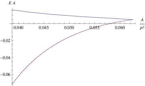
Of course, not all cross sections will do so, as illustrated in Fig. 9. This shows the trajectory of the Casimir energy for cylinders of rectangular cross section, written as a function of the variable . Here, the ratio of the sides of the rectangles can be written as
| (57) |
where , which takes on the maximum value of for a square. It will be noted that compared to what was found above for the triangles, the behavior of the rectangle energies is very different, changing from positive to negative at , which corresponds to .
Acknowledgements.
We thank the US Department of Energy (grant number DE-FG02-04ER41305) and the US National Science Foundation (grants number PHY-0968492 and PHY-0545390) for partial support of this research. We thank Steven Armour, Prachi Parashar, Nima Pourtolami, and Jef Wagner for collaborative assistance, and Steve Fulling for helpful comments.Appendix A Chowla-Selberg formula
Since it is relatively unfamiliar, in this appendix we sketch the derivation of the Chowla-Selberg formula from the Abel-Plana formula,
| (58) |
which requires that be analytic in the right half-plane. If is analytic in the left half-plane, we can derive the identical formula for
Now consider the sum
| (59) |
where the double prime means that the single term is omitted. We take
| (60) |
where so the sum exists. It is easy to show that
| (61) |
We apply the Abel-Plana formula to the two sums in Eq. (61), with the result
| (62) |
where
| (63a) | |||
| and | |||
| (63b) | |||
where the different terms have branch points in the 2nd, 3rd, 1st, and 4th quadrants, respectively.
It is rather easy to evaluate the integral II in terms of the integral
| (64) |
The end-point contributions cancel, with the result
| (65) |
where .
The final integral III is evaluated by shifting the contour by an imaginary amount (the shifts along the imaginary axis vanish) and encircling the branch point, so that we obtain
| III | (66) | ||||
which uses the representation of the modified Bessel function,
| (67) |
Using Eqs. (65) and (66) in Eq. (62), we find the Chowla-Selberg formula (8) with .
References
- [1] H. B. G. Casimir, Proc. Kon. Ned. Akad. Wetensch. 51, 793 (1948).
- [2] M. Y. Sparnaay, Physica 24, 751 (1958).
- [3] S. K. Lamoreaux, Phys. Rev. Lett. 78, 5 (1997).
- [4] U. Mohideen and A. Roy, Phys. Rev. Lett. 81, 4549 (1998).
- [5] R. S. Decca, D. Lopez, E. Fischbach, G. L. Klimchitskaya, D. E. Krause, and V. M. Mostepanenko, Ann. Phys. (NY) 318, 37 (2005).
- [6] T. H. Boyer, Phys. Rev. 174, 1764 (1968).
- [7] H. B. G. Casimir, Physica 19, 846 (1956).
- [8] W. Lukosz, Physica 56, 109 (1971).
- [9] J. Ambjørn and S. Wolfram, Ann. Phys. (NY) 147, 1 (1983).
- [10] L. L. DeRaad, Jr. and K. A. Milton, Ann. Phys. (NY) 136, 229 (1981).
- [11] P. Gosdzinsky and A. Romeo, Phys. Lett. B 441, 265 (1998).
- [12] E. Elizalde, S. D. Odintsov, A. Romeo, A. A. Bytsenko, and S. Zerbini, Zeta Regularization Techniques with Applications (World Scientific, 1994).
- [13] S. Chowla and A. Selberg, J. reine u. angewandte Math. 227, 86 (1967).
- [14] M. Lerch, Bull. sci. math. 21, 290 (1897).
- [15] L. Lorenz, Matematisk Tidsskrift 1, 97 (1871).
- [16] G. H. Hardy, Messenger Math. 49, 85 (1919).
- [17] A. Fletcher, J. C. P. Miller, L. Rosenhead, and L. J. Comrie, An Index of Mathematical Tables (Blackwell, London, 1962), Vol. 1, p. 95.
- [18] I. J. Zucker, J. Math. Phys. 15, 187 (1974).
- [19] M. L. Glasser and I. J. Zucker, Theoretical Chemistry: Advances and Perspectives (Academic, New York, 1980), Vol. 5, p. 67.
- [20] C. Itzykson and J. M. Luck, J. Phys. A 19, 211 (1986).
- [21] C. Itzykson, P. Moussa, and J. M. Luck, J. Phys. A 19, L111 (1986).
- [22] A. A. Kvitsinsky, J. Phys. A 29, 6379 (1996).
- [23] W. Lukosz, Z. Phys. 258, 99 (1973).
- [24] W. Lukosz, Z. Phys. 262, 327 (1973).
- [25] J. R. Ruggiero, A. H. Zimerman, and A. Villani, Rev. Bras. Fis. 7, 663 (1977).
- [26] J. R. Ruggiero, A. H. Zimerman, and A. Villani, J. Phys. A 13, 761 (1980).
- [27] K. A. Milton, A. V. Nesterenko, and V. V. Nesterenko, Phys. Rev. D59 105009 (1999).
- [28] N. Inui, J. Phys. Soc. Jap. 76, 11 (2007).
- [29] H. Ahmedov and I. H. Duru, J. Math. Phys. 45, 3 (2004).
- [30] R. D. Hazlett and D. K. Babu, Quart. Appl. Math. 67, 579 (2009).
- [31] E. Álvarez, F. D. Mazzitelli, A. G. Monastra, and D. A. Wisniacki, arXiv:1007.4742.
- [32] K. A. Milton and J. Schwinger, Electromagnetic Radiation: Variational Methods, Waveguides and Accelerators (Springer, 2006).
- [33] J. Schwinger, L. L. DeRaad, Jr., K. A. Milton, and W.-y. Tsai, Classical Electrodynamics (Westview Press, 1998).
- [34] K. A. Milton, arXiv:1005.0031 [hep-th].
- [35] J. A. Stratton, Electromagnetic Theory (McGraw-Hill, New York, 1941).
- [36] M. G. Lamé, Leçons sur la théorie mathématique de l’élasticité des corps solides (Bachelier, Paris, 1852).
- [37] E. Vergini and M. Saraceno, Phys. Rev. E 52, 2204 (1995).
- [38] A. H. Barnett, Comm. Pure Appl. Math. 59, 1457 (2006).
- [39] S. A. Fulling, L. Kaplan, and J. H. Wilson, Phys. Rev. A 76, 012118 (2007).
- [40] I. Cavero-Peláez, K. A. Milton, and K. Kirsten, J. Phys. A 40, 3607 (2007).
- [41] K. Kirsten, Spectral Functions in Mathematics and Physics (Chapman & Hall/CRC, Boca Raton, FL, 2001).
- [42] S. A. Fulling, J. Phys. A 36, 6857 (2003).
- [43] A. Pleijel, Ark. Mat. 2, 663 (1954).
- [44] M. Kac, Am. Math. Mon. 73, 1 (1966).
- [45] H. P. McKean and I. M. Singer, J. Diff. Geom. 1, 43 (1967).
- [46] S. Sen, Phys. Rev. D 24, 869 (1981).
- [47] S. Sen, J. Math. Phys. 22, 2968 (1981).