Fundamental Results on Fluid Approximations of Stochastic Process Algebra Models

Journal: Performance Evaluation

Jie Ding Email: jieding@yzu.edu.cn Address: School of Information Engineering, The University of Yangzhou, Yangzhou, China Jane Hillstion Email: jane.hillston@ed.ac.uk Address: Laboratory for Foundations of Computer Science, School of Informatics, The University of Edinburgh, Edinburgh, UK.

Abstract

In order to avoid the state space explosion problem encountered in the quantitative analysis of large scale PEPA models, a fluid approximation approach has recently been proposed, which results in a set of ordinary differential equations (ODEs) to approximate the underlying continuous time Markov chain (CTMC). This paper presents a mapping semantics from PEPA to ODEs based on a numerical representation scheme, which extends the class of PEPA models that can be subjected to fluid approximation. Furthermore, we have established the fundamental characteristics of the derived ODEs, such as the existence, uniqueness, boundedness and nonnegativeness of the solution. The convergence of the solution as time tends to infinity for several classes of PEPA models, has been proved under some mild conditions. For general PEPA models, the convergence is proved under a particular condition, which has been revealed to relate to some famous constants of Markov chains such as the spectral gap and the Log-Sobolev constant. This thesis has established the consistency between the fluid approximation and the underlying CTMCs for PEPA, i.e. the limit of the solution is consistent with the equilibrium probability distribution corresponding to a family of underlying density dependent CTMCs.

Keywords:

Fluid Approximation; PEPA; Convergence

1 Introduction

Stochastic process algebras, such as PEPA [1], TIPP [2], EMPA [3], IMC [4], are powerful modelling formalisms for concurrent systems which have enjoyed considerable success over the last decade. Such modeling can help designers and system managers by allowing aspects of a system which are not readily tested, such as scalability, to be analysed before a system is deployed. However, both model construction and analysis can be challenged by the size and complexity of large scale systems. This problem, called state space explosion, is inherent in the discrete state approach employed in stochastic process algebras and many other formal modelling approaches. To overcome this problem, many work devoted exploiting the compositionality of the process algebra to decompose or simplify the underlying CTMC e.g. [5, 6, 7, 8, 9, 10]. Another technique is the use of Kronecker algebra [11, 12, 13, 14]. In addition, abstract Markov chains and stochastic bounds techniques have also been used to analyse large scale PEPA models [15, 16].

The techniques reported above are based on the discrete state space. Therefore as the size of the state space is extremely large, these techniques are not always strong enough to handle the state space explosion problem. For example, in the modelling of biochemical mechanisms using the stochastic $\pi$ -calculus [17, 18] and PEPA [19, 20], the state space explosion problem becomes almost insurmountable. Consequently in many cases models are analysed by discrete event simulation rather than being able to abstractly consider all possible behaviours.

To avoid this problem Hillston proposed a radically different approach in [21] from the following two perspectives: choosing a more abstract state representation in terms of state variables, quantifying the types of behaviour evident in the model; and assuming that these state variables are subject to continuous rather than discrete change. This approach results in a set of ODEs, leading to the evaluation of transient, and in the limit, steady state measures.

However, there are not many discussions on the fundamental problems, such as the existence, uniqueness, boundedness and nonnegativeness of the solution, as well as the its asymptotic behaviour as time tends to infinity, and the relationship between the derived ODEs and the underlying CTMCs for general PEPA models. Solving these problems can not only bring confidence in the new approach, but can also provide new insight into, as well as a profound understanding of, performance formalisms. This paper will focus on these topics and give answers to these problems.

The remainder of this paper is structured as follows. Section 2 will give a brief introduction to PEPA as well as a numerical representation scheme developed for PEPA. Based on this scheme, the fluid approximation of PEPE models will be introduced in Section 3. In this section, the existence and uniqueness of solutions of the derived ODEs will be presented. In addition, we will show that for a PEPA model without synchronisations, the solution of the ODEs converges as time goes to infinity and the limit coincides with the steady-state probability distribution of the underlying CTMC. In Section 4, we demonstrate the consistency between the fluid approximation and the Markov chains underlying the same PEPA model. This relationship will be utilised to investigate the long-time behaviour of the ODEs’ solutions in Section 5. The convergence of the solutions will be proved under a particular condition, which relates the convergence problem to some well-known constants of Markov chains such as the spectral gap and the Log-Sobolev constant. Section 6 and 7 present an analytic approach to analyse the fluid approximation. For several classes of PEPA models, the convergence will be demonstrated under some mild conditions, and the coefficient matrices of the derived ODEs have been exposed to have the following property: all eigenvalues are either zeros or have negative real parts. In addition, the structural property of invariance in PEPA models will be shown to play an important role in the proof of convergence. Finally, after presenting some related work in Section 8, we conclude the paper in Section 9.

2 The PEPA modelling formalism

This section will briefly introduce the PEPA language and its numerical representation scheme. The numerical representation scheme for PEPA was developed by Ding in his thesis [22], and represents a model numerically rather than syntactically supporting the use of mathematical tools and methods to analyse the model.

2.1 Introduction to PEPA

PEPA (Performance Evaluation Process Algebra) [1], developed by Hillston in the 1990s, is a high-level model specification language for low-level stochastic models, and describes a system as an interaction of the components which engage in activities. In contrast to classical process algebras, activities are assumed to have a duration which is a random variable governed by an exponential distribution. Thus each activity in PEPA is a pair $(\alpha,r)$ where $\alpha$ is the action type and $r$ is the activity rate. The language has a small number of combinators, for which we provide a brief introduction below; the structured operational semantics can be found in [1]. The grammar is as follows:

	$\displaystyle S$	$\displaystyle::=$	$\displaystyle(\alpha,r).S\mid S+S\mid C_{S}$
	$\displaystyle P$	$\displaystyle::=$	$\displaystyle P\raisebox{-4.30554pt}{$\;\stackrel{{\scriptstyle\mbox{\large$\rhd\!\!\!\lhd$}}}{{\scriptscriptstyle L}}\,$}P\mid P/L\mid C$

where $S$ denotes a sequential component and $P$ denotes a model component which executes in parallel. $C$ stands for a constant which denotes either a sequential component or a model component as introduced by a definition. $C_{S}$ stands for constants which denote sequential components. The effect of this syntactic separation between these types of constants is to constrain legal PEPA components to be cooperations of sequential processes.

Prefix: The prefix component $(\alpha,r).S$ has a designated first activity $(\alpha,r)$ , which has action type $\alpha$ and a duration which satisfies exponential distribution with parameter $r$ , and subsequently behaves as $S$ .

Choice: The component $S+T$ represents a system which may behave either as $S$ or as $T$ . The activities of both $S$ and $T$ are enabled. Since each has an associated rate there is a race condition between them and the first to complete is selected. This gives rise to an implicit probabilistic choice between actions dependent of the relative values of their rates.

Hiding: Hiding provides type abstraction, but note that the duration of the activity is unaffected. In $P/L$ all activities whose action types are in $L$ appear as the “private” type $\tau$ .

Cooperation: $P\raisebox{-4.30554pt}{$\;\stackrel{{\scriptstyle\mbox{\large$\rhd\!\!\!\lhd$}}}{{\scriptscriptstyle L}}\,$}Q$ denotes cooperation between $P$ and $Q$ over action types in the cooperation set $L$ . The cooperands are forced to synchronise on action types in $L$ while they can proceed independently and concurrently with other enabled activities (individual activities). The rate of the synchronised or shared activity is determined by the slower cooperation (see [1] for details). We write $P\parallel Q$ as an abbreviation for $P\raisebox{-4.30554pt}{$\;\stackrel{{\scriptstyle\mbox{\large$\rhd\!\!\!\lhd$}}}{{\scriptscriptstyle L}}\,$}Q$ when $L=\emptyset$ and $P[N]$ is used to represent $N$ copies of $P$ in a parallel, i.e. $P[3]=P\parallel P\parallel P$ .

Constant: The meaning of a constant is given by a defining equation such as $A\stackrel{{\scriptstyle\mbox{{\tiny def}}}}{{=}}P$ . This allows infinite behaviour over finite states to be defined via mutually recursive definitions.

On the basis of the operational semantic rules (please refer to [1] for details), a PEPA model may be regarded as a labelled multi-transition system

\left(\mathcal{C},\mathcal{A}ct,\left\{\mathop{\longrightarrow}\limits^{(\alpha,r)}|(\alpha,r)\in\mathcal{A}ct\right\}\right)

where $\mathcal{C}$ is the set of components, $\mathcal{A}ct$ is the set of activities and the multi-relation $\mathop{\longrightarrow}\limits^{(\alpha,r)}$ is given by the rules. If a component $P$ behaves as $Q$ after it completes activity $(\alpha,r)$ , then denote the transition as $P\mathop{\longrightarrow}\limits^{(\alpha,r)}Q$ .

The memoryless property of the exponential distribution, which is satisfied by the durations of all activities, means that the stochastic process underlying the labelled transition system has the Markov property. Hence the underlying stochastic process is a CTMC. Note that in this representation the states of the system are the syntactic terms derived by the operational semantics. Once constructed the CTMC can be used to find steady state or transient probability distributions from which quantitative performance can be derived.

2.2 Numerical Representation of PEPA Models

As explained above there have been two key steps in the use of fluid approximation for PEPA models: firstly, the shift to a numerical vector representation of the model, and secondly, the use of ordinary differential equations to approximate the dynamic behaviour of the underlying CTMC. In this paper we are only concerned with the former modification.

This section presents the numerical representation of PEPA models developed in [22]. For convenience, we may represent a transition $P\stackrel{{\scriptstyle(\alpha,r)}}{{\longrightarrow}}Q$ as $P\stackrel{{\scriptstyle(\alpha,r_{\alpha}^{P\rightarrow Q})}}{{\longrightarrow}}Q$ , or often simply as $P\stackrel{{\scriptstyle\alpha}}{{\longrightarrow}}Q$ since the rate is not pertinent to structural analysis, where $P$ and $Q$ are two local derivatives. Following [21], hereafter the term local derivative refers to the local state of a single sequential component. In the standard structured operational semantics of PEPA used to derive the underlying CTMC, the state representation is syntactic, keeping track of the local derivative of each component in the model. In the alternative numerical vector representation some information is lost as states only record the number of instances of each local derivative:

Definition 1.

(Numerical Vector Form [21]). For an arbitrary PEPA model $\mathcal{M}$ with $n$ component types ${C}_{i},i=1,2,\cdots,n$ , each with $d_{i}$ distinct local derivatives, the numerical vector form of $\mathcal{M}$ , $\mathbf{m}(\mathcal{M})$ , is a vector with $d=\sum_{i=1}^{n}d_{i}$ entries. The entry $\mathbf{m}[{C}_{i_{j}}]$ records how many instances of the $j$ th local derivative of component type ${C}_{i}$ are exhibited in the current state.

In the following we will find it useful to distinguish derivatives according to whether they enable an activity, or are the result of that activity:

Definition 2.

(Pre and post local derivative)

1.

If a local derivative $P$ can enable an activity $\alpha$ , that is $P\mathop{\longrightarrow}\limits^{\alpha}\cdot$ , then $P$ is called a pre local derivative of $\alpha$ . The set of all pre local derivatives of $\alpha$ is denoted by $\mathrm{pre}(\alpha)$ , called the pre set of $\alpha$ .
2.

If $Q$ is a local derivative obtained by firing an activity $\alpha$ , i.e. $\cdot\mathop{\longrightarrow}\limits^{\alpha}Q$ , then $Q$ is called a post local derivative of $\alpha$ . The set of all post local derivatives is denoted by $\mathrm{post}(\alpha)$ , called the post set of $\alpha$ .
3.

The set of all the local derivatives derived from $P$ by firing $\alpha$ , i.e.

$\mathrm{post}(P,\alpha)=\{Q\mid P\stackrel{{\scriptstyle\alpha}}{{\longrightarrow}}Q\},$

is called the post set of $\alpha$ from $P$ .

Within a PEPA model there may be many instances of the same activity type but we will wish to identify those that have exactly the same effect within the model. In order to do this we additionally label activities according to the derivatives to which they relate, giving rise to labelled activities:

Definition 3.

(Labelled Activity).

1.

For any individual activity $\alpha$ , for each $P\in\mathrm{pre}(\alpha),Q\in\mathrm{post}(P,\alpha)$ , label $\alpha$ as $\alpha^{P\rightarrow Q}$ .

For a shared activity $\alpha$ , for each $(Q_{1},Q_{2},\cdots,Q_{k})$ in

\mathrm{post}(\mathrm{pre}(\alpha)[1],\alpha)\times\mathrm{post}(\mathrm{pre}(\alpha)[2],\alpha)\times\cdots\times\mathrm{post}(\mathrm{pre}(\alpha)[k],\alpha),

label $\alpha$ as $\alpha^{w}$ , where

w=(\mathrm{pre}(\alpha)[1]\rightarrow Q_{1},\mathrm{pre}(\alpha)[2]\rightarrow Q_{2},\cdots,\mathrm{pre}(\alpha)[k]\rightarrow Q_{k}).

Each $\alpha^{P\rightarrow Q}$ or $\alpha^{w}$ is called a labelled activity. The set of all labelled activities is denoted by $\mathcal{A}_{\mbox{\small label }}$ . For the above labelled activities $\alpha^{P\rightarrow Q}$ and $\alpha^{w}$ , their respective pre and post sets are defined as

\mathrm{pre}(\alpha^{P\rightarrow Q})=\{P\},\;\mathrm{post}(\alpha^{P\rightarrow Q})=\{Q\},

\mathrm{pre}(\alpha^{w})=\mathrm{pre}(\alpha),\;\mathrm{post}(\alpha^{w})=\{Q_{1},Q_{2},\cdots,Q_{k}\}.

In the numerical representation scheme, the transitions between states of the model are represented by a matrix, termed the activity matrix — this records the impact of the labelled activities on the local derivatives.

Definition 4.

(Activity Matrix, Pre Activity Matrix, Post Activity Matrix). For a model with $N_{\mathcal{A}_{\mbox{\small label }}}$ labelled activities and $N_{\mathcal{D}}$ distinct local derivatives, the activity matrix $\mathbf{C}$ is an $N_{\mathcal{D}}\times N_{\mathcal{A}_{\mbox{\small label }}}$ matrix, and the entries are defined as following

\mathbf{C}(P_{i},\alpha_{j})=\left\{\begin{array}[]{ll}+1&\mbox{if }\;\;P_{i}\in\mathrm{post}(\alpha_{j})\\ -1&\mbox{if }\;\;P_{i}\in\mathrm{pre}(\alpha_{j})\\ 0&\mbox{otherwise}\end{array}\right.

where $\alpha_{j}$ is a labelled activity. The pre activity matrix $\mathbf{C^{pre}}$ and post activity matrix $\mathbf{C^{post}}$ are defined as

\mathbf{C^{Pre}}(P_{i},\alpha_{j})=\left\{\begin{array}[]{ll}+1&\mbox{if }\;\;P_{i}\in\mathrm{pre}(\alpha_{j})\\ 0&\mbox{otherwise}.\end{array}\right.,

\mathbf{C^{Post}}(P_{i},\alpha_{j})=\left\{\begin{array}[]{ll}+1&\mbox{if }\;\;P_{i}\in\mathrm{post}(\alpha_{j})\\ 0&\mbox{otherwise}.\end{array}\right.

From Definitions 3 and 4, each column of the activity matrix corresponds to a system transition and each transition can be represented by a column of the activity matrix. The activity matrix equals the difference between the pre and post activity matrices, i.e. $\mathbf{C=C^{Post}-C^{Pre}}$ . The rate of the transition between states is specified by a transition rate function, but we omit this detail here since we are concerned with qualitative analysis. See [22] for details.

We first give the definition of the apparent rate of an activity in a local derivative.

Definition 5.

(Apparent Rate of $\alpha$ in $P$ ) Suppose $\alpha$ is an activity of a PEPA model and $P$ is a local derivative enabling $\alpha$ (i.e. $P\in\mathrm{pre}(\alpha)$ ). Let $\mathrm{post}(P,\alpha)$ be the set of all the local derivatives derived from $P$ by firing $\alpha$ , i.e. $\mathrm{post}(P,\alpha)=\{Q\mid P\stackrel{{\scriptstyle(\alpha,r_{\alpha}^{P\rightarrow Q})}}{{\longrightarrow}}Q\}.$ Let

r_{\alpha}(P)=\sum_{Q\in\mathrm{post}(P,\alpha)}r_{\alpha}^{P\rightarrow Q}.

(1)

The apparent rate of $\alpha$ in $P$ in state $\mathbf{x}$ , denoted by $r_{\alpha}(\mathbf{x},P)$ , is defined as

r_{\alpha}(\mathbf{x},P)=\mathbf{x}[P]r_{\alpha}(P).

(2)

The above definition is used to define the following transition rate function.

Definition 6.

(Transition Rate Function) Suppose $\alpha$ is an activity of a PEPA model and $\mathbf{x}$ denotes a state vector.

1.

If $\alpha$ is individual, then for each $P\stackrel{{\scriptstyle(\alpha,r^{P\rightarrow Q})}}{{\longrightarrow}}Q$ , the transition rate function of labelled activity $\alpha^{P\rightarrow Q}$ in state $\mathbf{x}$ is defined as

$f(\mathbf{x},\alpha^{P\rightarrow Q})=\mathbf{x}[P]r_{\alpha}^{P\rightarrow Q}.$ (3)

If $\alpha$ is synchronised, with $\mathrm{pre}(\alpha)=\{P_{1},P_{2},\cdots,P_{k}\}$ , then for each

(Q_{1},Q_{2},\cdots,Q_{k})\in\mathrm{post}(P_{1},\alpha)\times\mathrm{post}(P_{2},\alpha)\times\cdots\times\mathrm{post}(P_{k},\alpha),

let $w=(P_{1}\rightarrow Q_{1},P_{2}\rightarrow Q_{2},\cdots,P_{k}\rightarrow Q_{k})$ . Then the transition rate function of labelled activity $\alpha^{w}$ in state $\mathbf{x}$ is defined as

f(\mathbf{x},\alpha^{w})=\left(\prod_{i=1}^{k}\frac{r_{\alpha}^{P_{i}\rightarrow Q_{i}}}{r_{\alpha}(P_{i})}\right)\min_{i\in\{1,\cdots,k\}}\{r_{\alpha}(\mathbf{x},P_{i})\},

where $r_{\alpha}(\mathbf{x},P_{i})=\mathbf{x}[P_{i}]r_{\alpha}(P_{i})$ is the apparent rate of $\alpha$ in $P_{i}$ in state $\mathbf{x}$ . So

f(\mathbf{x},\alpha^{w})=\left(\prod_{i=1}^{k}\frac{r_{\alpha}^{P_{i}\rightarrow Q_{i}}}{r_{\alpha}(P_{i})}\right)\min_{i\in\{1,\cdots,k\}}\{\mathbf{x}[P_{i}]r_{\alpha}(P_{i})\}.

(4)

Note that Definition 6 accommodates the passive or unspecified rate $\top$ . An algorithm for automatically deriving the numerical representation of a PEPA model was presented in [22].

Remark 1.

Definition 6 accommodates the passive or unspecified rate $\top$ . If there are some $r^{U\rightarrow V}_{l}$ which are $\top$ , then the relevant calculation in the rate functions (3) and (4) can be made according to the following inequalities and equations that define the comparison and manipulation of unspecified activity rates (see Section 3.3.5 in [1]):

\begin{array}[]{cl}r<w\top&\emph{\mbox{for all $r\in\mathbb{R}^{+}$ and for all $w\in\mathbb{N}$}}\\ w_{1}\top<w_{2}\top&\emph{\mbox{if $w_{1}<w_{2}$ for all $w_{1},w_{2}\in\mathbb{N}$}}\\ w_{1}\top+w_{2}\top=(w_{1}+w_{2})\top&\emph{\mbox{for all $w_{1},w_{2}\in\mathbb{N}$}}\\ \frac{w_{1}\top}{w_{2}\top}=\frac{w_{1}}{w_{2}}&\emph{\mbox{for all $w_{1},w_{2}\in\mathbb{N}$}}\end{array}

Moreover, we assume that $0\cdot\top=0$ . So the terms such as “ $\min\{A\top,rB\}$ ” are interpreted as [23]:

\min\{A\top,rB\}=\left\{\begin{array}[]{cc}rB,&A>0,\\ 0,&A=0.\end{array}\right.

The transition rate function has the following properties [22]:

Proposition 1.

The transition rate function is nonnegative; if $P$ is a pre local derivative of $l$ , i.e. $P\in\mathrm{pre}(l)$ , then the transition rate function of $l$ in a state $\mathbf{x}$ is less than the apparent rate of $l$ in $U$ in this state, that is

0\leq f(\mathbf{x},l)\leq r_{l}(\mathbf{x},P)=\mathbf{x}[P]r_{l}(P),

where $r_{l}(P)$ is the apparent rate of $l$ in $P$ for a single instance of $P$ .

Proposition 2.

Let $l$ be an labelled activity, and $\mathbf{x,y}$ be two states. The transition rate function $f(\mathbf{x},l)$ defined in Definition 6 satisfies:

1.

For any $H>0$ , $Hf(\mathbf{x}/H,l)=f(\mathbf{x},l)$ .
2.

There exists $M>0$ such that $|f(\mathbf{x},l)-f(\mathbf{y},l)|\leq M\|\mathbf{x}-\mathbf{y}\|$ for any $\mathbf{x},\mathbf{y}$ and $l$ .

Hereafter $\|\cdot\|$ denotes any matrix norm since all finite matrix norms are equivalent. The first term of this proposition illustrates a homogenous property of the rate function, while the second indicates the Lipschtiz continuous property, both with respect to states.

3 Fluid approximations for PEPA models

The section will introduce the fluid-flow approximations for PEPA models, which leads to some kind of nonlinear ODEs. The existence and uniqueness of the solutions of the ODEs will be established. Moreover, a conservation law satisfied by the ODEs will be shown.

3.1 State space explosion problem: an illustration by a tiny example

Let us first consider the following tiny example.

Model 1.

\begin{split}User_{1}\stackrel{{\scriptstyle\mbox{{\tiny def}}}}{{=}}&(task_{1},a).User_{2}\\ User_{2}\stackrel{{\scriptstyle\mbox{{\tiny def}}}}{{=}}&(task_{2},b).User_{1}\\ Provider_{1}\stackrel{{\scriptstyle\mbox{{\tiny def}}}}{{=}}&(task_{1},a).Provider_{2}\\ Provider_{2}\stackrel{{\scriptstyle\mbox{{\tiny def}}}}{{=}}&(reset,d).Provider_{1}\\ \underbrace{User_{1}||\cdots||User_{1}}_{\mbox{$M$ copies}}&\raisebox{-4.30554pt}{$\;\stackrel{{\scriptstyle\mbox{\large$\rhd\!\!\!\lhd$}}}{{\scriptscriptstyle\{task1\}}}\,$}\underbrace{Provider_{1}||\cdots||Provider_{1}}_{\mbox{$N$ copies}}\end{split}

According to the semantics of PEPA originally defined in [1], the size of the state space of the CTMC underlying Model 1 is $2^{M+N}$ . That is, the size of the state space increases exponentially with the numbers of the users and providers in the system. Consequently, the dimension of the infinitesimal generator of the CTMC is $2^{M+N}\times 2^{M+N}$ . The computational complexity of solving the global balance equation to get the steady-state probability distribution and thus derive the system performance, is therefore exponentially increasing with the numbers of the components. When $M$ and/or $N$ are large, the calculation of the stationary probability distribution will be infeasible due to limited resources of memory and time. The problem encountered here is the so-called state-space explosion problem.

A model aggregation technique, i.e. representing the states by numerical vector forms, which is introduced by Gilmore et al. in [24] and by Hillston in [21], can help to relieve the state-space explosion problem. It has been proved in [22] that by employing numerical vector forms the size of the state space can be reduced to $2^{M}\times 2^{N}$ to $(M+1)\times(N+1)$ , without relevant information and accuracy loss. However, this does not imply there is no complexity problem. The following table, Table 1, gives the runtimes of deriving the state space in several different scenarios. All experiments were carried out using the PEPA Plug-in (v0.0.19) for Eclipse Platform (v3.4.2), on a 2.66GHz Xeon CPU with 4Gb RAM running Scientific Linux 5. The runtimes here are elapsed times reported by the Eclipse platform.

Table 1: Elapsed time of state pace derivation

$(M,N)$	(300,300)	(350,300)	(400,300)	(400,400)
time	$2879$ ms	4236 ms	“Java heap space"	“GC overhead limit exceeded"

If there are 400 users and 300 providers in the system, the Eclipse platform reports the error message of “Java heap space", while 400 users and 400 providers result in the error information of “GC overhead limit exceeded". These experiments show that the state-space explosion problem cannot be completely solved by just using the technique of numerical vector form, even for a tiny PEPA model. That is, in order to do practical analysis for large scale PEPA models we need new approaches.

3.2 Fluid approximation of PEPA models

In the numerical representation of PEPA presented in Section 2.2, a numerical vector form is introduced to capture the state information of models with repeated components. In this vector form there is one entry for each local derivative of each component type in the model. The entries in the vector are no longer syntactic terms representing the local derivative of the sequential component, but the number of components currently exhibiting this local derivative. Each numerical vector represents a single state of the system. The rates of the transitions between states are specified by the transition rate functions. For example, the transition from state $\mathbf{x}$ to $\mathbf{x}+l$ can be written as

\mathbf{x}\mathop{\longrightarrow}\limits^{(l,f(\mathbf{x},l))}\mathbf{x}+l,

where $l$ is a transition vector corresponding to the labelled activity $l$ (for convenience, hereafter each pair of transition vectors and corresponding labelled activities shares the same notation), and $f(\mathbf{x},l)$ is the transition rate function, reflecting the intensity of the transition from $\mathbf{x}$ to $\mathbf{x}+l$ .

The state space is inherently discrete with the entries within the numerical vector form always being non-negative integers and always being incremented or decremented in steps of one. As pointed out in [21], when the numbers of components are large these steps are relatively small and we can approximate the behaviour by considering the movement between states to be continuous, rather than occurring in discontinuous jumps. In fact, let us consider the evolution of the numerical state vector. Denote the state at time $t$ by $\mathbf{x}(t)$ . In a short time $\Delta t$ , the change to the vector $\mathbf{x}(t)$ will be

\mathbf{x}(\cdot,t+\Delta t)-\mathbf{x}(\cdot,t)=F(\mathbf{x}(\cdot,t))\Delta t=\Delta t\sum_{l\in\mathcal{A}_{\mathrm{label}}}lf(\mathbf{x}(\cdot,t),l).

Dividing by $\Delta t$ and taking the limit, $\Delta t\rightarrow 0$ , we obtain a set of ordinary differential equations (ODEs):

\frac{\mathrm{d}\mathbf{x}}{\mathrm{d}t}=F(\mathbf{x}),

(5)

where

F(\mathbf{x})=\sum_{l\in\mathcal{A}_{\mathrm{label}}}lf(\mathbf{x},l).

(6)

Once the activity matrix and the transition rate functions are generated, the ODEs are immediately available. All of them can be obtained automatically by a derivation algorithm presented in [22].

Let $U$ be a local derivative. For any transition vector $l$ , $l[U]$ is either $\pm 1$ or $0$ . If $l[U]=-1$ then $U$ is in the pre set of $l$ , i.e. $U\in\mathrm{pre}(l)$ , while $l[U]=1$ implies $U\in\mathrm{post}(l)$ . According to (5) and (6),

\begin{split}\frac{\mathrm{d}\mathbf{x}(U,t)}{\mathrm{d}t}&=\sum_{l}l[U]f(\mathbf{x},l)\\ &=-\sum_{l:l[U]=-1}f(\mathbf{x},l)+\sum_{l:l[U]=1}f(\mathbf{x},l)\\ &=-\sum_{\{l\mid U\in\mathrm{pre}(l)\}}\!\!\!\!f(\mathbf{x},l)+\sum_{\{l\mid U\in\mathrm{post}(l)\}}\hskip-8.53581ptf(\mathbf{x},l).\end{split}

(7)

The term $\sum_{\{l\mid U\in\mathrm{pre}(l)\}}\hskip 0.0ptf(\mathbf{x},l)$ represents the “exit rates” in the local derivative $U$ , while the term $\sum_{\{l\mid U\in\mathrm{post}(l)\}}\hskip 0.0ptf(\mathbf{x},l)$ reflects the “entry rates” in $U$ . The formulae (5) and (6) are activity centric while (7) is local derivative centric. Our approach to derive ODEs has extended previous results presented in the literature [21, 23, 25], by relaxing restrictions such as allowing shared activities may have different local rates, each action name may appear in different local derivatives within the definition of a sequential component, and may occur multiple times with that derivative definition, etc.

For an arbitrary CTMC, the evolution of probabilities distributed on each state can be described by a set of linear ODEs ([26], page 52). For example, for the (aggregated) CTMC underlying a PEPA model, the corresponding differential equations describing the evolution of the probability distributions are

\frac{\mathrm{d}\mathbf{\pi}}{\mathrm{d}t}=Q^{T}\mathbf{\pi},

(8)

where each entry of $\mathbf{\pi}(t)$ represents the probability of the system being in each state at time $t$ , and $Q$ is an infinitesimal generator matrix corresponding to the CTMC. Clearly, the dimension of the coefficient matrix $Q$ is the square of the size of the state space, which increases as the number of components increases.

The derived ODEs (5) describe the evolution of the population of the components in each local derivative, while (8) reflects the the probability evolution at each state. Since the scale of (5), i.e. the number of the ODEs, is only determined by the number of local derivatives and is unaffected by the size of the state space, so it avoids the state-space explosion problem. But the scale of (8) depends on the size of the state space, so it suffers from the explosion problem. The price paid is that the ODEs (5) are generally nonlinear due to synchronisations, while (8) is linear. However, if there is no synchronisation contained then (5) becomes linear, and there is some correspondence and consistency between these two different types of ODEs, which will be demonstrated in Section 3.4.

3.3 Existence and uniqueness of ODEs’ solution

For any set of ODEs, it is important to consider if the equations have a solution, and if so whether that solution is unique.

Theorem 1.

For a given PEPA model without passive rates, the derived ODEs from this model have a unique solution in the time interval $[0,\mathchar 561\relax)$ .

Proof.

Notice that each entry of $F(\mathbf{x})=\sum_{l}lf(\mathbf{x},l)$ is a linear combination of the transition rate functions $f(\mathbf{x},l)$ , so $F(\mathbf{x})$ is globally Lipschitz continuous since each $f(\mathbf{x},l)$ is globally Lipschitz continuous. That is, there exits $M>0$ such that $\forall\mathbf{x},\mathbf{y}$ ,

||F(\mathbf{x})-F(\mathbf{y})||\leq M||\mathbf{x}-\mathbf{y}||.

(9)

By the classical theory in ODEs (e.g. Theorem 6.2.3 in [27], page 14), the derived ODEs have a unique solution in $[0,\mathchar 561\relax)$ . ∎

As we have mentioned, in the formula (7), the term $\sum_{\{l\mid U\in\mathrm{pre}(l)\}}\hskip 0.0ptf(\mathbf{x},l)$ represents the exit rates in the local derivative $U$ , while the term $\sum_{\{l\mid U\in\mathrm{post}(l)\}}\hskip 0.0ptf(\mathbf{x},l)$ reflects the entry rates in $U$ . For each type of component at any time, the sum of all exit activity rates must be equal to the sum of all entry activity rates, since the system is closed and there is no exchange with the environment. This leads to the following proposition.

Proposition 3.

Let $C_{i_{j}}$ be a local derivative of component type $C_{i}$ . Then for any $i$ and $t$ , $\displaystyle\sum_{j}\frac{\mathrm{d}\mathbf{x}\left(C_{i_{j}},t\right)}{\mathrm{d}t}=0$ , and $\sum_{j}\mathbf{x}\left(C_{i_{j}},t\right)=\sum_{j}\mathbf{x}\left(C_{i_{j}},0\right).$

Proof.

In the definition of activity matrix, the numbers of $-1$ and $1$ appearing in the entries of any transition vector $l$ (i.e. a column of the activity matrix), which correspond to the component type $C_{i}$ , are the same [22], i.e.

\#\{j:l[C_{i_{j}}]=-1\}=\#\{j:l[C_{i_{j}}]=1\}.

(10)

Let $\mathbf{y}$ be an indicator vector with the same dimension as $l$ satisfying:

\mathbf{y}[{C}_{i_{j}}]=\left\{\begin{array}[]{cl}1,&\mathrm{if}\;l[{C}_{i_{j}}]=\pm 1,\\ 0,&\mathrm{otherwise.}\end{array}\right.

So $\mathbf{y}^{T}l=0$ by (10). Thus

\mathbf{y}^{T}\frac{\mathrm{d}\mathbf{x}}{\mathrm{d}t}=\mathbf{y}^{T}\sum_{l}lf(\mathbf{x},l)=\sum_{l}\mathbf{y}^{T}lf(\mathbf{x},l)=0.

That is, $\displaystyle\sum_{j}\frac{\mathrm{d}\mathbf{x}\left(C_{i_{j}},t\right)}{\mathrm{d}t}=\mathbf{y}^{T}\frac{\mathrm{d}\mathbf{x}}{\mathrm{d}t}=0.$ So $\sum_{j}\mathbf{x}\left(C_{i_{j}},t\right)$ is a constant and equal to $\sum_{j}\mathbf{x}\left(C_{i_{j}},0\right)$ , i.e. the number of the copies of component type $C_{i}$ in the system initially. ∎

Proposition 3 means that the ODEs satisfy a Conservation Law, i.e. the number of each kind of component remains constant at all times.

3.4 Convergence and consistence of ODEs’ solution: nonsynchronised models

Now we consider PEPA models without synchronisation. For this special class of PEPA models, we will show that the solutions of the derived ODEs have finite limits. Moreover, the limits coincide with the steady-state probability distributions of the underlying CTMCs.

3.4.1 Features of ODEs without synchronisations

Suppose the PEPA model has no synchronisations. Without loss of generality, we suppose that there is only one kind of component $C$ in the system. In fact, if there are several types of component in the system, the ODEs related to the different types of component can be separated and treated independently since there are no interactions between them. Thus, we assume there is only one kind of component $C$ and that $C$ has $k$ local derivatives: $C_{1},C_{2},\cdots,C_{k}$ . Then (5) is

\begin{split}\frac{\mathrm{d}\left(\mathbf{x}(C_{1},t),\cdots,\mathbf{x}(C_{k},t)\right)^{T}}{\mathrm{d}t}=\sum_{l}lf(\mathbf{x},l).\end{split}

(11)

Since (11) are linear ODEs, we may rewrite (11) as the following matrix form:

\frac{\mathrm{d}\left(\mathbf{x}(C_{1},t),\cdots,\mathbf{x}(C_{k},t)\right)^{T}}{\mathrm{d}t}=Q^{T}\left(\mathbf{x}(C_{1},t),\cdots,\mathbf{x}(C_{k},t)\right)^{T},

(12)

where $Q=\left(q_{ij}\right)$ is a $k\times k$ matrix.

$Q$ has many good properties.

Proposition 4.

$Q=\left(q_{ij}\right)_{k\times k}$ in (12) is an infinitesimal generator matrix, that is, $\left(q_{ij}\right)_{k\times k}$ satisfies

1.

$0\leq-q_{ii}<\mathchar 561\relax$ for all $i$ ;
2.

$q_{ij}\geq 0$ for all $i\neq j$ ;
3.

$\sum_{j=1}^{k}q_{ij}=0$ for all $i$ .

Proof.

According to (12), we have

\frac{\mathrm{d}\mathbf{x}(C_{i},t)}{\mathrm{d}t}=\sum_{j=1}^{k}\mathbf{x}(C_{j},t)q_{ji}.

(13)

Notice by (7),

\frac{\mathrm{d}\mathbf{x}(C_{i},t)}{\mathrm{d}t}=-\sum_{\{l\mid C_{i}\in\mathrm{pre}(l)\}}\!\!\!\!f(\mathbf{x},l)+\sum_{\{l\mid C_{i}\in\mathrm{post}(l)\}}\hskip-8.53581ptf(\mathbf{x},l).

\sum_{j=1}^{k}\mathbf{x}(C_{j},t)q_{ji}=-\sum_{\{l\mid C_{i}\in\mathrm{pre}(l)\}}\!\!\!\!f(\mathbf{x},l)+\sum_{\{l\mid C_{i}\in\mathrm{post}(l)\}}\hskip-8.53581ptf(\mathbf{x},l).

(14)

Since there is no synchronisation in the system, the transition function $f(\mathbf{x},l)$ is linear with respect to $\mathbf{x}$ and therefore there is no nonlinear term,“ $\min$ ”, in it. In particular, if $C_{i}\in\mathrm{pre}(l)$ , then $f(\mathbf{x},l)=r_{l}(C_{i})\mathbf{x}[C_{i}]$ , which is the apparent rate of $l$ in $C_{i}$ in state $\mathbf{x}$ defined in Definition 5. We should point out that according to our semantics of mapping PEPA models to ODEs, the fluid approximation-version of $f(\mathbf{x},l)$ also holds, i.e. $f(\mathbf{x}(t),l)=r_{l}(C_{i})\mathbf{x}(C_{i},t)$ . So (14) becomes

\mathbf{x}(C_{i},t)q_{ii}+\sum_{j\neq i}\mathbf{x}(C_{j},t)q_{ji}=\mathbf{x}(C_{i},t)\sum_{\{l\mid C_{i}\in\mathrm{pre}(l)\}}\hskip-8.53581pt\left(-r_{l}(C_{i})\right)+\sum_{\{l\mid C_{i}\in\mathrm{post}(l)\}}\hskip-8.53581ptf(\mathbf{x},l).

(15)

Moreover, as long as $f(\mathbf{x},l)=r_{l}(C_{i})\mathbf{x}(C_{i})$ for some $l$ and some positive constants $r_{l}(C_{i})$ , which implies that $l$ can be fired at $C_{i}$ , we must have $C_{i}\in\mathrm{pre}(l)$ . That is to say, if $C_{i}\in\mathrm{post}(l)$ then $f(\mathbf{x},l)$ cannot be of the form of $r\mathbf{x}(C_{i},t)$ for any constant $r>0$ . Otherwise, we have $C_{i}\in\mathrm{pre}(l)$ , which results a contradiction¹¹ 1 In this paper we do not allow a self-loop in the considered model. That is, any PEPA definition like “ $C\stackrel{{\scriptstyle\mbox{{\tiny def}}}}{{=}}(\alpha,r).C$ ” which results in $C\in\mathrm{pre}(\alpha)$ and $C\in\mathrm{post}(\alpha)$ simultaneously, is not allowed. to $C_{i}\in\mathrm{post}(l)$ . So according to (15), we have

\mathbf{x}(C_{i},t)q_{ii}=\mathbf{x}(C_{i},t)\sum_{\{l\mid C_{i}\in\mathrm{pre}(l)\}}\hskip-8.53581pt\left(-r_{l}(C_{i})\right),

(16)

\sum_{j\neq i}\mathbf{x}(C_{j},t)q_{ji}=\sum_{\{l\mid C_{i}\in\mathrm{post}(l)\}}\hskip-8.53581ptf(\mathbf{x},l).

(17)

Thus by (16), $q_{ii}=\sum_{\{l\mid C_{i}\in\mathrm{pre}(l)\}}\left(-r_{l}(C_{i})\right)$ , and $0\leq-q_{ii}<\mathchar 561\relax$ for all $i$ . Item 1 is proved.

Similarly, for any $C_{j},\;j\neq i$ , if $f(\mathbf{x},l)=r\mathbf{x}(C_{j},t)$ for some $l$ and positive constant $r$ , then clearly $C_{j}$ is in the pre set of $l$ . That is $C_{j}\in\mathrm{pre}(l)$ . So by (17),

\mathbf{x}(C_{j},t)q_{ji}=\sum_{\{l\mid C_{j}\in\mathrm{pre}(l),C_{i}\in\mathrm{post}(l)\}}\hskip-8.53581ptf(\mathbf{x},l)=\mathbf{x}(C_{j},t)\sum_{l}r_{l}^{C_{j}\rightarrow C_{i}},

(18)

which implies $q_{ji}=\sum_{l}r_{l}^{C_{j}\rightarrow C_{i}}\geq 0$ for all $i\neq j$ , i.e. item 2 holds.

We now prove item 3. By Proposition 3,

\frac{\mathbf{x}(C_{1},t)}{dt}+\frac{\mathbf{x}(C_{2},t)}{dt}+\cdots+\frac{\mathbf{x}(C_{k},t)}{dt}=0.

(19)

Then by (13) and (19), for all $t$ ,

\begin{split}&\mathbf{x}(C_{1},t)\sum_{j=1}^{k}q_{1j}+\mathbf{x}(C_{2},t)\sum_{j=1}^{k}q_{2j}+\cdots+\mathbf{x}(C_{k},t)\sum_{j=1}^{k}q_{kj}\\ =&\sum_{i=1}^{k}\mathbf{x}(C_{i},t)\sum_{j=1}^{k}q_{ij}=\sum_{j=1}^{k}\sum_{i=1}^{k}\mathbf{x}(C_{i},t)q_{ij}=\sum_{j=1}^{k}\frac{\mathrm{d}\mathbf{x}(C_{j},t)}{\mathrm{d}t}=0.\end{split}

This implies $\sum_{j=1}^{k}q_{ij}=0$ for all $i$ . ∎

In the proof of Proposition 4, we have shown the relationship between the coefficient matrix $Q$ and the activity rates:

q_{ii}=-\sum_{\{l\mid C_{i}\in\mathrm{pre}(l)\}}r_{l}(C_{i}),\quad q_{ij}=\sum_{l}r_{l}^{C_{i}\rightarrow C_{j}}\;(i\neq j).

We point out that this infinitesimal generator matrix $Q_{k\times k}$ may not be the infinitesimal generator matrix of the CTMC derived via the usual semantics of PEPA (we call it the “original" CTMC for convenience). In fact, the original CTMC has a state space with $k^{N}$ states and the dimension of its infinitesimal generator matrix is $k^{N}\times k^{N}$ , where $N$ is the total number of components in the system. However, this $Q_{k\times k}$ is the infinitesimal generator matrix of a CTMC underlying the PEPA model in which there is only one copy of the component, i.e. $N=1$ . To distinguish this from the original one, we refer to this CTMC as the “singleton” CTMC.

3.4.2 Convergence and consistency for the ODEs

Proposition 4 illustrates that the coefficient matrix of the derived ODEs is an infinitesimal generator. If there is only one component in the system, then equation (12) captures the probability distribution evolution equations of the original CTMC. Based on this proposition, we can furthermore determine the convergence of the solutions.

Theorem 2.

Suppose $\mathbf{x}\left(C_{j},t\right)\;(j=1,2,\cdots,k)$ satisfy (11), then for any given initial values $\mathbf{x}\left(C_{j},0\right)\geq 0\;(j=1,2,\cdots,k)$ , there exist constants $\mathbf{x}(C_{j},\mathchar 561\relax)$ , such that

\lim_{t\rightarrow\mathchar 561\relax}\mathbf{x}(C_{j},t)=\mathbf{x}(C_{j},\mathchar 561\relax),\quad j=1,2,\cdots,k.

(20)

Proof.

By Proposition 4, the matrix $Q$ in (12) is an infinitesimal generator matrix. Consider a “singleton” CTMC which has the state space $S=\{C_{1},C_{2},\cdots,C_{k}\}$ , the infinitesimal generator matrix $Q$ in (12) and the initial probability distribution $\mathbf{\pi}(C_{j},0)=\frac{\mathbf{x}(C_{j},0)}{N}\;(j=1,2,\cdots,k)$ . Then according to Markov theory ([26], page 52), $\mathbf{\pi}(C_{j},t)\;(j=1,2,\cdots,k)$ , the probability distribution of this new CTMC at time $t$ , satisfies

\frac{\mathrm{d}\left(\mathbf{\pi}(C_{1},t),\cdots,\mathbf{\pi}(C_{k},t)\right)}{\mathrm{d}t}=\left(\mathbf{\pi}(C_{1},t),\cdots,\mathbf{\pi}(C_{k},t)\right)Q

(21)

Since the singleton CTMC is assumed irreducible and positive-recurrent, it has a steady-state probability distribution $\{\mathbf{\pi}(C_{j},\mathchar 561\relax)\}_{j=1}^{k}$ , and

\lim_{t\rightarrow\mathchar 561\relax}\mathbf{\pi}(C_{j},t)=\mathbf{\pi}(C_{j},\mathchar 561\relax),\quad j=1,2,\cdots,k.

(22)

Note that $\frac{\mathbf{x}(C_{j},t)}{N}$ also satisfies (21) with the initial values $\frac{\mathbf{x}(C_{j},0)}{N}$ equal to $\mathbf{\pi}(C_{j},0)$ , where $N$ is the population of the components. By the uniqueness of the solutions of (21), we have

\frac{\mathbf{x}(C_{j},t)}{N}=\mathbf{\pi}(C_{j},t),\quad j=1,2,\cdots,k,

(23)

and hence by (22),

\lim_{t\rightarrow\mathchar 561\relax}\mathbf{x}(C_{j},t)=\lim_{t\rightarrow\mathchar 561\relax}N\mathbf{\pi}(C_{j},t)=N\mathbf{\pi}(C_{j},\mathchar 561\relax),\quad j=1,2,\cdots,k.

∎

Clearly, if there are multiple types of component in the system, then Theorem 2 holds for each each component type, since there is no cooperation between different component types and they can be treated independently.

It is shown in [28] that for some special examples the equilibrium solutions of the ODEs coincide with the steady state probability distributions of the underlying original CTMC. This theorem states that this holds for all for PEPA models without synchronisations. Moreover, it is also exposed by this theorem that the fluid approximation is consistent with the CTMC underlying the same nonsynchronised PEPA model.

4 Relating to density dependent CTMCs

A general PEPA model may have synchronisations, which result in the nonlinearity of the derived ODEs. However, it is difficult to rely on pure analytical methods to explore the asymptotic behaviour of the solution of the derived ODEs from an arbitrary PEPA model (except for some special classes of models, see the next two sections).

Fortunately, Kurtz’s theorem [29, 30] establishes the relationship between a sequence of Markov chains and a corresponding set of ODEs: the complete solution of some ODEs is the limit of a sequence of Markov chains. In the context of PEPA, the derived ODEs can be considered as the limit of pure jump Markov processes, as first exposed in [25] for a special case. Thus we may investigate the convergence of the ODEs’ solutions by alternatively studying the corresponding property of the Markov chains through this consistency relationship. This approach leads to the result presented in the next section: under a particular condition the solution will converge and the limit is consistent with the limit steady-state probability distribution of a family of CTMCs underlying the given PEPA model. Let us first introduce the concept of density dependent Markov chains underlying PEPA models.

4.1 Density dependent Markov chains underlying PEPA models

In the numerical state vector representation scheme, each vector is a single state and the rates of the transitions between states are specified by the rate functions. For example, the transition from state $\mathbf{x}$ to $\mathbf{x}+l$ can be written as

\mathbf{x}\mathop{\longrightarrow}\limits^{(l,f(\mathbf{x},l))}\mathbf{x}+l.

Since all the transitions are only determined by the current state rather than the previous ones, given any starting state a CTMC can be obtained. More specifically, the state space of the CTMC is the set of all reachable numerical state vectors $\mathbf{x}$ . The infinitesimal generator is determined by the transition rate function,

q_{\mathbf{x},\mathbf{x}+l}=f(\mathbf{x},l).

(24)

Because the transition rate function is defined according to the semantics of PEPA, the CTMC mentioned above is in fact the aggregated CTMC underlying the given PEPA model. In other words, the transition rate of the aggregated CTMC is specified by the transition rate function in Definition 6.

It is obvious that the aggregated CTMC depends on the starting state of the given PEPA model. By altering the population of components presented in the model, which can be done by varying the initial states, we may get a sequence of aggregated CTMCs. Moreover, Proposition 2 indicates that the transition rate function has the homogenous property: $Hf(\mathbf{x}/H,l)=f(\mathbf{x},l),\linebreak\forall H>0$ . This property identifies the aggregated CTMC to be density dependent.

Definition 7.

[29]. A family of CTMCs $\{X_{n}\}_{n}$ is called density dependent if and only if there exists a continuous function $f(\mathbf{x},l),\;\mathbf{x}\in\mathbb{R}^{d},\;l\in\mathbb{Z}^{d}$ , such that the infinitesimal generators of $X_{n}$ are given by:

q^{(n)}_{\mathbf{x},\mathbf{x}+l}=nf(\mathbf{x}/n,l),\quad l\neq 0,

where $q^{(n)}_{\mathbf{x},\mathbf{x}+l}$ denotes an entry of the infinitesimal generator of $X_{n}$ , $\mathbf{x}$ a numerical state vector and $l$ a transition vector.

This allows us to conclude the following proposition.

Proposition 5.

Let $\{X_{n}\}$ be a sequence of aggregated CTMCs generated from a given PEPA model (by scaling the initial state), then $\{X_{n}\}$ is density dependent.

Proof.

For any $n$ , the transition between states is determined by

q^{(n)}_{\mathbf{x},\mathbf{x}+l}=f(\mathbf{x},l),

where $\mathbf{x},\mathbf{x}+l$ are state vectors, $l$ corresponds to an activity, $f(\mathbf{x},l)$ is the rate of the transition from state $\mathbf{x}$ to $\mathbf{x}+l$ . By Proposition 2,

nf(\mathbf{x}/n,l)=f(\mathbf{x},l).

So the infinitesimal generator of $X_{n}$ is given by:

q^{(n)}_{\mathbf{x},\mathbf{x}+l}=f(\mathbf{x},l)=nf(\mathbf{x}/n,l),\quad l\neq 0.

Therefore, $\{X_{n}\}$ is a sequence of density dependent CTMCs. ∎

In particular, the family of density dependent CTMCs, $\{X_{n}(t)\}$ , derived from a given PEPA model with the starting condition $X_{n}(0)=n\mathbf{x}_{0}\;(\forall n)$ , is called the density dependent CTMCs associated with $\mathbf{x}_{0}$ . The CTMCs $\frac{X_{n}(t)}{n}$ are called the concentrated density dependent CTMCs. Here $n$ is called the concentration level, indicating that the entries within the numerical vector states (of $\frac{X_{n}(t)}{n}$ ) are incremented and decremented in steps of $\frac{1}{n}$ .

For example, Consider the following PEPA model, which is Model 1 presented previously:

\begin{split}User_{1}\stackrel{{\scriptstyle\mbox{{\tiny def}}}}{{=}}&(task_{1},a).User_{2}\\ User_{2}\stackrel{{\scriptstyle\mbox{{\tiny def}}}}{{=}}&(task_{2},b).User_{1}\\ Provider_{1}\stackrel{{\scriptstyle\mbox{{\tiny def}}}}{{=}}&(task_{1},a).Provider_{2}\\ Provider_{2}\stackrel{{\scriptstyle\mbox{{\tiny def}}}}{{=}}&(reset,d).Provider_{1}\\ (User_{1}[M])&\raisebox{-4.30554pt}{$\;\stackrel{{\scriptstyle\mbox{\large$\rhd\!\!\!\lhd$}}}{{\scriptscriptstyle\{task1\}}}\,$}(Provider_{1}[N]).\end{split}

The activity matrix and transition rate functions have been specified in Table 2. In this table, $U_{i},P_{i}\;(i=1,2)$ are the local derivatives representing $User_{i}$ and $Provider_{i}$ respectively. For convenience, the labelled activities or transition vectors ${task_{1}}^{(U_{1}\rightarrow U_{2},P_{1}\rightarrow P_{2})}$ , $task_{2}^{U_{2}\rightarrow U_{1}}$ , ${reset}^{P_{2}\rightarrow P_{1}}$ will subsequently be denoted by $l^{task_{1}},l^{task_{2}},l^{reset}$ respectively.

Table 2: Activity matrix and transition rate function of Model 1

$l$	${task_{1}}^{(U_{1}\rightarrow U_{2},P_{1}\rightarrow P_{2})}$	$task_{2}^{U_{2}\rightarrow U_{1}}$	${reset}^{P_{2}\rightarrow P_{1}}$
$U_{1}$	$-1$	1	0
$U_{2}$	1	$-1$	0
$P_{1}$	$-1$	0	1
$P_{2}$	1	0	$-1$
$f(\mathbf{x},l)$	$a\min(\mathbf{x}[U_{1}],\mathbf{x}[P_{1}])$	$b\mathbf{x}[U_{2}]$	$d\mathbf{x}[P_{2}]$

Suppose $\mathbf{x}_{1}=(M,0,N,0)^{T}=(1,0,1,0)^{T}$ . Let $X_{1}(t)$ be the aggregated CTMC underlying Model 1 with initial state $\mathbf{x}_{1}$ . Then the state space of $X_{1}(t)$ , denoted by $S_{1}$ , is composed of

\begin{split}\begin{array}[]{ll}\mathbf{x}_{1}=(1,0,1,0)^{T},&\mathbf{x}_{2}=(0,1,0,1)^{T},\\ \mathbf{x}_{3}=(1,0,0,1)^{T},&\mathbf{x}_{4}=(0,1,1,0)^{T}.\\ \end{array}\end{split}

(25)

According to the transition rate functions presented in Table 2, we have, for instance,

q^{(1)}_{\mathbf{x}_{1},\mathbf{x}_{2}}=q_{\mathbf{x}_{1},\mathbf{x}_{1}+l^{task_{1}}}=f(\mathbf{x}_{1},l^{task_{1}})=a\min(\mathbf{x}_{1}[U_{1}],\mathbf{x}_{1}[P_{1}])=a.

Varying the initial states we may get other aggregated CTMCs. For example, let $X_{2}(t)$ be the aggregated CTMC corresponding to the initial state $X_{2}(0)=2\mathbf{x}_{0}=(2,0,2,0)^{T}$ . Then the state space $S_{2}$ of $X_{2}(t)$ has the states

\begin{split}\begin{array}[]{lll}\mathbf{x}_{1}=(2,0,2,0)^{T},&\mathbf{x}_{2}=(1,1,1,1)^{T},&\mathbf{x}_{3}=(1,1,2,0)^{T},\\ \mathbf{x}_{4}=(1,1,0,2)^{T},&\mathbf{x}_{5}=(0,2,1,1)^{T},&\mathbf{x}_{6}=(2,0,1,1)^{T},\\ \mathbf{x}_{7}=(0,2,0,2)^{T},&\mathbf{x}_{8}=(0,2,2,0)^{T},&\mathbf{x}_{9}=(2,0,0,2)^{T}.\end{array}\end{split}

(26)

The rate of transition from $\mathbf{x}_{1}$ to $\mathbf{x}_{2}$ is determined by

q^{(2)}_{\mathbf{x}_{1},\mathbf{x}_{2}}=q_{\mathbf{x}_{1},\mathbf{x}_{1}+l^{task_{1}}}=f(\mathbf{x}_{1},l^{task_{1}})=2a=2f(\mathbf{x}_{1}/2,l^{task_{1}}).

Similarly, let $X_{n}(t)$ be the aggregated CTMC corresponding to the initial state $X_{n}(0)=n\mathbf{x}_{0}$ . Then the transition from $\mathbf{x}$ to $\mathbf{x}+l$ is determined by

q^{(n)}_{\mathbf{x},\mathbf{x}+l}=f(\mathbf{x},l)=nf(\mathbf{x}/n,l).

Thus a family of aggregated CTMCs, i.e. $\{X_{n}(t)\}$ , has been obtained from Model 1. These derived $\{X_{n}(t)\}$ are density dependent CTMCs associated with $\mathbf{x}_{0}$ . As illustrated by this example, the density dependent CTMCs are obtained by scaling the starting state $\mathbf{x}_{0}$ . So the starting state of each CTMC is different, because $X_{n}(0)=n\mathbf{x}_{0}$ , i.e. $X_{n}(0)=n(M,0,N,0)^{T}$ .

4.2 Fluid approximation as the limit of the CTMCs

As discussed above, a set of ODEs and a sequence of density dependent Markov chains can be derived from the same PEPA model. The former one is deterministic while the latter is stochastic. However, both of them are determined by the same activity matrix and the same rate functions that are uniquely generated from the given PEPA model. Therefore, it is natural to believe that there is some kind of consistency between them.

As we have mentioned, the complete solution of some ODEs can be the limit of a sequence of Markov chains according to Kurtz’s theorem [29, 30]. Such consistency in the context of PEPA has been previously illustrated for a particular PEPA model [25]. Here we give a modified version of this result for general PEPA models, in which the convergence is in the sense of almost surely rather than probabilistically as in [25].

Theorem 3.

Let $X(t)$ be the solution of the ODEs (5) derived from a given PEPA model with initial condition $\mathbf{x}_{0}$ , and let $\{X_{n}(t)\}$ be the density dependent CTMCs associated with $\mathbf{x}_{0}$ underlying the same PEPA model. Let $\hat{X}_{n}(t)=\frac{X_{n}(t)}{n}$ , then for any $t>0$ ,

\lim_{n\rightarrow\mathchar 561\relax}\sup_{u\leq t}\|\hat{X}_{n}(u)-X(u)\|=0\quad\quad a.s.

(27)

Proof.

According to Kurtz’s theorem, which is listed in A, it is sufficient to prove: for any compact set $K\subset\mathbb{R}^{N_{d}}$ ,

1.

$\exists M_{K}>0$ such that $\|F(\mathbf{x})-F(\mathbf{y})\|\leq M_{K}\|\mathbf{x}-\mathbf{y}\|$ ;
2.

$\sum_{l}\|l\|\sup_{\mathbf{x}\in K}f(\mathbf{x},l)<\mathchar 561\relax$ .

Clearly, above term 1 is satisfied. Since $f(\mathbf{x},l)$ is continuous by Proposition 2, it is bounded on any compact $K$ . Notice that any entry of $l$ takes values in $\{1,-1,0\}$ , so $\|l\|$ is bounded. Thus term 2 is satisfied, which completes the proof. ∎

Theorem 3 allows us to investigate the properties of $X(t)$ through studying the characteristics of the family of CTMCs $\hat{X}_{n}(t)=\frac{X_{n}(t)}{n}$ . Notice that $X_{n}(t)$ takes values in the state space which corresponds to the starting state $n\mathbf{x}_{0}$ . Clearly, each state of $\hat{X}_{n}(t)$ is bounded and nonnegative (more precisely, each entry in any numerical state vector is nonnegative, and bounded by $\|\mathbf{x}_{0}\|$ according to the conservative law). So the ODEs’ solution $X(t)$ inherits these characteristics since $X(t)$ is the limit of $\hat{X}_{n}(t)$ as $n$ goes to infinity. That is, $X(t)$ is bounded and nonnegative. The proof is trivial and omitted here. Instead, a purely analytic proof of these properties will be given in Section 6.1.

4.3 Consistency between the fluid approximation and the CTMCs

As shown in Theorem 3, for a given PEPA model with synchronisations, the derived ODEs can be taken as the underlying density dependent CTMC with the concentration level infinity. If the given model has no synchronisations, then by Proposition 4 and the proof of Theorem 2, the ODEs coincide the probability distribution evolution equations of the CTMC with the concentration level one, except for a scaling factor. These two conclusions embody the consistency between the fluid approximation and the CTMCs for PEPA models. Moreover, as we will see in the next section, the limit of the ODEs’ solution as time tends to infinity (if it exists) is consistent with the limit of the expectations of the corresponding CTMCs.

However, it is natural to ask such a question: for a PEPA model with synchronisations, since the ODEs corresponds the CTMC with the concentration level infinity and our performance evaluation is based on the usual underlying CTMC, i.e. the CTMC with the concentration level one, what is the loss brought by using the fluid approximation approach? Although in the sense of concentration level there is a gap between one and infinity, but in practice for large scale synchronised models (i.e. models with a large number of repetitive components), the relative errors of performance measure such as throughput and average response time between the concentration level one and infinity are usually small enough to be ignored (i.e. less than $5\%$ ) [22]. Therefore, it is safe to employ the fluid approximation for large scale models.

This paper more likely concentrates on the long-time behaviour the ODEs’ solution. In the following sections, we focus on the problem of whether the ODEs’ solution converges as time goes to problem will be presented in the next section, which is based on the consistency relationship between the derived ODEs and the CTMCs revealed in Theorem 3.

5 Convergence of ODEs’ solution: a probabilistic approach

Analogous to the steady-state probability distributions of the Markov chains underlying PEPA models, upon which performance measures such as throughput and utilisation can be derived, we expect the solution of the generated ODEs to have similar equilibrium conditions. In particular, if the solution has a limit as time goes to infinity we will be able to similarly obtain the performance from the steady state, i.e. the limit. Therefore, whether the solution of the derived ODEs converges becomes an important problem.

We should point out that Kurtz’s theorem cannot directly apply to the problem of whether or not the solution the derived ODEs converges. This is because Kurtz’s theorem only deals with the approximation between the ODEs and Markov chains during any finite time, rather than considering the asymptotic behaviour of the ODEs as time goes to infinity. This section will present our investigation and results about this problem.

5.1 Convergence under a particular condition

We follow the assumptions in Theorem 3. Denote the expectation of $\hat{X}_{n}(t)$ as $\hat{M}_{n}(t)$ , i.e. $\hat{M}_{n}(t)=E[\hat{X}_{n}(t)]$ . For any $t$ , the stochastic processes $\{\hat{X}_{n}(t)\}_{n}$ converge to the deterministic $X(t)$ when $n$ tends to infinity, as Theorem 3 shows. It is not surprising to see that $\{\hat{M}_{n}(t)\}_{n}$ , the expectations of $\{\hat{X}_{n}(t)\}_{n}$ , also converge to $X(t)$ as $n\rightarrow\mathchar 561\relax$ :

Lemma 1.

For any $t$ ,

\lim_{n\rightarrow\mathchar 561\relax}\hat{M}_{n}(t)=X(t).

Proof.

Since $X(t)$ is deterministic, then $E[X(t)]=X(t)$ . By Theorem 3, for all $t$ , $\hat{X}_{n}(t)$ converges to $X(t)$ almost surely as $n$ goes to infinity. Notice that $\hat{X}_{n}(t)$ is bounded (see the discussion in the previous section), then by Lebesgue’s dominant convergence theorem, we have

\lim_{n\rightarrow\mathchar 561\relax}E\|\hat{X}_{n}(t)-X(t)\|=0.

\begin{split}\lim_{n\rightarrow\mathchar 561\relax}\|\hat{M}_{n}(t)-X(t)\|&=\lim_{n\rightarrow\mathchar 561\relax}\|E[\hat{X}_{n}(t)]-E[X(t)]\|\\ &\leq\lim_{n\rightarrow\mathchar 561\relax}E\|\hat{X}_{n}(t)-X(t)\|\\ &=0.\end{split}

∎

Lemma 1 states that the ODEs’ solution $X(t)$ is just the limit function of the sequence of the expectation functions of the corresponding density dependent Markov chains. This provides some clues: the characteristics of the limit $X(t)$ depend on the properties of $\{\hat{M}_{n}(t)\}_{n}$ . Therefore, we expect to be able to investigate $X(t)$ by studying $\{\hat{M}_{n}(t)\}_{n}$ .

Since $\hat{M}_{n}(t)$ is the expectation of the Markov chain $\hat{X}_{n}(t)$ , $\hat{M}_{n}(t)$ can be expressed by a formula in which the transient probability distribution is involved. That is,

\hat{M}_{n}(t)=E[\hat{X}_{n}(t)]=\sum_{\mathbf{x}\in\hat{S}_{n}}\mathbf{x}\hat{\mathbf{\pi}}^{n}_{t}(\mathbf{x}),

where $\hat{S}_{n}$ is the state space, $\hat{\mathbf{\pi}}^{n}_{t}(\cdot)$ is the probability distribution of $\hat{X}_{n}$ at time $t$ . Let ${S}_{n}$ and $\mathbf{\pi}^{n}_{t}(\cdot)$ be the state space and the probability distribution of $X_{n}(t)$ respectively²² 2 We should point out that the probability distributions of $X_{n}(t)$ and $\hat{X}_{n}(t)$ are the same, i.e. $\mathbf{\pi}^{n}_{t}(\mathbf{x})=\hat{\mathbf{\pi}}^{n}_{t}(\mathbf{x}/n)$ .. Then

\hat{M}_{n}(t)=E[\hat{X}_{n}(t)]=E\left[\frac{X_{n}(t)}{n}\right]=\sum_{\mathbf{x}\in S^{n}}\frac{\mathbf{x}}{n}\mathbf{\pi}^{n}_{t}(\mathbf{x}).

We have assumed the Markov chains underlying PEPA models to be irreducible and positive-recurrent. Then the transient probability distributions of these Markov chains will converge to the corresponding steady-state probability distributions. We denote the steady-state probability distributions of $X_{n}(t)$ and $\hat{X}_{n}(t)$ as $\mathbf{\pi}^{n}_{\mathchar 561\relax}(\cdot)$ and $\hat{\mathbf{\pi}}^{n}_{\mathchar 561\relax}(\cdot)$ respectively. Then, we have a lemma.

Lemma 2.

For any $n$ , there exists a $\hat{M}_{n}(\mathchar 561\relax)$ , such that

\lim_{t\rightarrow\mathchar 561\relax}\hat{M}_{n}(t)=\hat{M}_{n}(\mathchar 561\relax).

Proof.

\begin{split}&\lim_{t\rightarrow\mathchar 561\relax}\hat{M}_{n}(t)\\ =&\lim_{t\rightarrow\mathchar 561\relax}\sum_{\mathbf{x}\in{S}_{n}}\frac{\mathbf{x}}{n}\mathbf{\pi}^{n}_{t}(\mathbf{x})=\sum_{\mathbf{x}\in{S}_{n}}\lim_{t\rightarrow\mathchar 561\relax}\frac{\mathbf{x}}{n}\mathbf{\pi}^{n}_{t}(\mathbf{x})=\sum_{\mathbf{x}\in{S}_{n}}\frac{\mathbf{x}}{n}\mathbf{\pi}^{n}_{\mathchar 561\relax}(\mathbf{x})\equiv\hat{M}_{n}(\mathchar 561\relax).\end{split}

∎

Clearly, we also have $\hat{M}_{n}(\mathchar 561\relax)=\sum_{\mathbf{x}\in\hat{S}_{n}}\mathbf{x}\hat{\mathbf{\pi}}^{n}_{\mathchar 561\relax}(\mathbf{x})$ .

Remark 2.

Currently, we do not know whether the sequence $\{\hat{M}_{n}(\mathchar 561\relax)\}_{n}$ converges as $n\rightarrow\mathchar 561\relax$ . But since $\{\hat{M}_{n}(\mathchar 561\relax)\}_{n}$ is bounded which is due to the conservation law that PEPA models satisfy, there exists $\{n^{\prime}\}\subset\{n\}$ such that $\{\hat{M}_{n^{\prime}}(\mathchar 561\relax)\}$ converges to a limit, namely $\hat{M}_{\mathchar 561\relax}(\mathchar 561\relax)$ . That is

\lim_{n^{\prime}\rightarrow\mathchar 561\relax}\hat{M}_{n^{\prime}}(\mathchar 561\relax)=\hat{M}_{\mathchar 561\relax}(\mathchar 561\relax).

Thus,

\lim_{n^{\prime}\rightarrow\mathchar 561\relax}\lim_{t\rightarrow\mathchar 561\relax}\hat{M}_{n^{\prime}}(t)=\lim_{n^{\prime}\rightarrow\mathchar 561\relax}\hat{M}_{n^{\prime}}(\mathchar 561\relax)=\hat{M}_{\mathchar 561\relax}(\mathchar 561\relax).

(28)

At the moment, there are two questions:

1.

Whether $\lim_{t\rightarrow\mathchar 561\relax}\lim_{n^{\prime}\rightarrow\mathchar 561\relax}\hat{M}_{n^{\prime}}(t)$ exists?

If $\lim_{t\rightarrow\mathchar 561\relax}\lim_{n^{\prime}\rightarrow\mathchar 561\relax}\hat{M}_{n^{\prime}}(t)$ exists, whether

\lim_{t\rightarrow\mathchar 561\relax}\lim_{n^{\prime}\rightarrow\mathchar 561\relax}\hat{M}_{n^{\prime}}(t)=\lim_{n^{\prime}\rightarrow\mathchar 561\relax}\lim_{t\rightarrow\mathchar 561\relax}\hat{M}_{n^{\prime}}(t)?

If the answer to the first question is yes, then the solution of the ODEs converges, since by Lemma 2, $\lim_{t\rightarrow\mathchar 561\relax}X(t)=\lim_{t\rightarrow\mathchar 561\relax}\lim_{n^{\prime}\rightarrow\mathchar 561\relax}\hat{M}_{n^{\prime}}(t).$ If the answer to the second question is yes, then the limit of $X(t)$ is consistent with the stationary distributions of the Markov chains since

\lim_{t\rightarrow\mathchar 561\relax}X(t)=\lim_{t\rightarrow\mathchar 561\relax}\lim_{n^{\prime}\rightarrow\mathchar 561\relax}\hat{M}_{n^{\prime}}(t)=\lim_{n^{\prime}\rightarrow\mathchar 561\relax}\lim_{t\rightarrow\mathchar 561\relax}\hat{M}_{n^{\prime}}(t)=\hat{M}_{\mathchar 561\relax}(\mathchar 561\relax).

In short, the positive answers to these two questions determine the convergence and consistency for the ODEs’s solution, see Figure 1. Fortunately, the two answers can be guaranteed by the condition (29) in the following Proposition 6.

Figure 1: Convergence and consistency diagram for derived ODEs

\begin{CD}\hat{M}_{n^{\prime}}(t)@>{n^{\prime}\rightarrow\mathchar 561\relax}>{\text{ \hskip 8.92513ptLemma~\ref{lem:Mn(t)=X(t)} \hskip 8.92513pt}}>X(t)(=\hat{M}_{\mathchar 561\relax}(t))\\ @V{t\rightarrow\mathchar 561\relax}V{\text{Lemma~\ref{lem:ChFP-Mn(t)Converges-Tconverges}}}V@V{{\Huge\color[rgb]{1,0,0}???}}V{t\rightarrow\mathchar 561\relax}V\\ \hat{M}_{n^{\prime}}(\mathchar 561\relax)@>{\text{\hskip 8.92513ptRemark~\ref{remark:M_{nk}limits} \hskip 8.92513pt}}>{n^{\prime}\rightarrow\mathchar 561\relax}>\hat{M}_{\mathchar 561\relax}(\mathchar 561\relax)\end{CD}

Proposition 6.

(A particular condition) If there exist $A,B>0$ , such that

\sup_{n^{\prime}}\left\|\hat{M}_{n^{\prime}}(t)-\hat{M}_{n^{\prime}}(\mathchar 561\relax)\right\|<Be^{-At},

(29)

then $\lim_{t\rightarrow\mathchar 561\relax}X(t)=\hat{M}_{\mathchar 561\relax}(\mathchar 561\relax)$ .

Proof.

$\displaystyle\left\\|X(t)-\hat{M}_{\mathchar 561\relax}(\mathchar 561\relax)\right\\|$	$\displaystyle=$	$\displaystyle\left\\|\lim_{n^{\prime}\rightarrow\mathchar 561\relax}[\hat{M}_{n^{\prime}}(t)-\hat{M}_{n^{\prime}}(\mathchar 561\relax)]\right\\|$
	$\displaystyle\leq$	$\displaystyle\limsup_{n^{\prime}\rightarrow\mathchar 561\relax}\left\\|\hat{M}_{n^{\prime}}(t)-\hat{M}_{n^{\prime}}(\mathchar 561\relax)\right\\|$
	$\displaystyle\leq$	$\displaystyle\limsup_{n^{\prime}\rightarrow\mathchar 561\relax}\left[\sup_{n^{\prime}}\left\\|\hat{M}_{n^{\prime}}(t)-\hat{M}_{n^{\prime}}(\mathchar 561\relax)\right\\|\right]$
	$\displaystyle\leq$	$\displaystyle\limsup_{n^{\prime}\rightarrow\mathchar 561\relax}Be^{-At}$
	$\displaystyle=$	$\displaystyle Be^{-At}\longrightarrow 0,\mbox{as }t\longrightarrow\mathchar 561\relax.$

So $\lim_{t\rightarrow\mathchar 561\relax}X(t)=\hat{M}_{\mathchar 561\relax}(\mathchar 561\relax)$ . ∎

Notice that $\displaystyle\hat{M}_{n}(t)=\sum_{\mathbf{x}\in S^{n}}\frac{\mathbf{x}}{n}\mathbf{\pi}^{n}_{t}(\mathbf{x})$ and $\displaystyle\hat{M}_{n}(\mathchar 561\relax)=\sum_{\mathbf{x}\in S^{n}}\frac{\mathbf{x}}{n}\mathbf{\pi}^{n}_{\mathchar 561\relax}(\mathbf{x})$ , so in order to estimate $\left\|\hat{M}_{n}(t)-\hat{M}_{n}(\mathchar 561\relax)\right\|$ in (29), we need first to estimate the difference between $\mathbf{\pi}^{n}_{t}$ and $\mathbf{\pi}^{n}_{\mathchar 561\relax}$ .

Lemma 3.

If there exists $A>0$ and $B_{1}>0$ , such that for any $n^{\prime}$ and all $\mathbf{x}\in S^{n^{\prime}}$ ,

|\mathbf{\pi}^{n^{\prime}}_{t}(\mathbf{x})-\mathbf{\pi}^{n^{\prime}}_{\mathchar 561\relax}(\mathbf{x})|\leq\mathbf{\pi}^{n^{\prime}}_{\mathchar 561\relax}(\mathbf{x})B_{1}e^{-At},

(30)

then there exists $B>0$ such that $\sup_{n^{\prime}}\left\|\hat{M}_{n^{\prime}}(t)-\hat{M}_{n^{\prime}}(\mathchar 561\relax)\right\|<Be^{-At}$ holds.

Proof.

We know that $\displaystyle\hat{X}_{n}(0)=\frac{{X}_{n}(0)}{n}=\mathbf{x}_{0}$ for any $n$ . By the conservation law, the population of each entity in any state is determined by the starting state. So for any $n^{\prime}$ and all $\mathbf{x}\in S^{n^{\prime}}$ , $||\mathbf{x}/{n^{\prime}}||\leq C_{1}\sum_{P\in\mathcal{D}}\mathbf{x}_{0}[P]<\mathchar 561\relax$ , where $\mathcal{D}$ is the set of all local derivatives and $C_{1}$ is a constant independent of $n^{\prime}$ . Let $C=\sup_{n^{\prime}}\max_{\mathbf{x}\in S^{n^{\prime}}}||\mathbf{x}/{n^{\prime}}||$ , then $C<\mathchar 561\relax$ .

$\displaystyle\left\\|\hat{M}_{n^{\prime}}(t)-\hat{M}_{n^{\prime}}(\mathchar 561\relax)\right\\|$	$\displaystyle=$	$\displaystyle\left\\|\sum_{\mathbf{x}\in S^{n^{\prime}}}\frac{\mathbf{x}}{n^{\prime}}\mathbf{\pi}^{n^{\prime}}_{t}(\mathbf{x})-\sum_{\mathbf{x}\in S^{n^{\prime}}}\frac{\mathbf{x}}{n^{\prime}}\mathbf{\pi}^{n^{\prime}}_{\mathchar 561\relax}(\mathbf{x})\right\\|$
	$\displaystyle=$	$\displaystyle\left\\|\sum_{\mathbf{x}\in S^{n^{\prime}}}\frac{\mathbf{x}}{n^{\prime}}(\mathbf{\pi}^{n^{\prime}}_{t}(\mathbf{x})-\mathbf{\pi}^{n^{\prime}}_{\mathchar 561\relax}(\mathbf{x}))\right\\|$
	$\displaystyle\leq$	$\displaystyle\sup_{n^{\prime}}\max_{\mathbf{x}\in S^{n^{\prime}}}\left\\|\frac{\mathbf{x}}{n^{\prime}}\right\\|\sum_{\mathbf{x}\in S^{n^{\prime}}}\|\mathbf{\pi}^{n^{\prime}}_{t}(\mathbf{x})-\mathbf{\pi}^{n^{\prime}}_{\mathchar 561\relax}(\mathbf{x})\|$
	$\displaystyle=$	$\displaystyle C\sum_{\mathbf{x}\in S^{n^{\prime}}}\|\mathbf{\pi}^{n^{\prime}}_{t}(\mathbf{x})-\pi^{n^{\prime}}_{\mathchar 561\relax}(\mathbf{x})\|$
	$\displaystyle\leq$	$\displaystyle C\sum_{\mathbf{x}\in S^{n^{\prime}}}\mathbf{\pi}^{n^{\prime}}_{\mathchar 561\relax}(\mathbf{x})B_{1}e^{-tA}$
	$\displaystyle=$	$\displaystyle CB_{1}e^{-tA}.$

Let $B=CB_{1}$ . Then $\sup_{n^{\prime}}\left\|\hat{M}_{n^{\prime}}(t)-\hat{M}_{n^{\prime}}(\mathchar 561\relax)\right\|<Be^{-At}$ . ∎

5.2 Investigation of the particular condition

This section will present the study of the particular condition (29). We will expose that the condition is related to well-known constants of Markov chains such as the spectral gap and the Log-Sobolev constant. The methods and results developed in the field of functional analysis of Markov chains are utilised to investigate the condition.

5.2.1 Important estimation for Markov kernel

We first give an estimation for the Markov kernel which is defined below. Let $Q$ be the infinitesimal generator of a Markov chain $X$ on a finite state $S$ . Let

K_{ij}=\left\{\begin{array}[]{cc}\frac{Q_{ij}}{m},&i\neq j\\ 1+\frac{Q_{ii}}{m},&i=j\\ \end{array}\right.\quad\mbox{where }m=\sup_{i}(-Q_{ii}).

$K$ is a transition probability matrix, satisfying

K(\mathbf{x},\mathbf{y})\geq 0,\quad\quad\sum_{\mathbf{y}}K(\mathbf{x},\mathbf{y})=1.

$K$ is called an Markov kernel ( $K$ is also called the uniformisation of the CTMC in some literature). A Markov chain on a finite state space $S$ can be described through its kernel $K$ . The continuous time semigroup associated with $K$ is defined by

H_{t}=\exp(-t(I-K)).

Let $\mathbf{\pi}$ be the unique stationary measure of the Markov chain. Then $H_{t}(\mathbf{x},\mathbf{y})\rightarrow\mathbf{\pi}(\mathbf{y})$ as $t$ tends to infinity. Following the convention in the literature we will also use $(K,\mathbf{\pi})$ to represent a Markov chain.

Notice

Q=m(K-I),\quad\quad K=\frac{Q}{m}+I.

Clearly,

P_{t}=e^{tQ}=e^{mt(K-I)}=e^{-mt(I-K)}=H_{mt},

and thus $H_{t}=P_{\frac{t}{m}}$ , where $P_{t}$ is called the semigroup associated with the infinitesimal generator $Q$ . An estimation of $H_{t}$ is given below.

Lemma 4.

(Corollary 2.2.6, [32]) Let $(K,\mathbf{\pi})$ be a finite Markov chain, and $\displaystyle\mathbf{\pi}(*)=\min_{\mathbf{x}\in S}{\mathbf{\pi}(\mathbf{x})}$ . Then

\sup_{\mathbf{x},\mathbf{y}}\left|\frac{H_{t}(\mathbf{x},\mathbf{y})}{\mathbf{\pi}(\mathbf{y})}-1\right|\leq e^{2-c}\;\quad\mbox{for }\;t=\frac{1}{\alpha}\log\log\frac{1}{\mathbf{\pi}(*)}+\frac{c}{\lambda},

(31)

where $\lambda>0,\alpha>0$ are the spectral gap and the Log-Sobolev constant respectively, which are defined and interpreted in B.

It can be implied from (31) that $\forall\mathbf{x},\mathbf{y}\in S$ ,

\left|{H_{t}(\mathbf{x},\mathbf{y})}-{\mathbf{\pi}(\mathbf{y})}\right|\leq\mathbf{\pi}(\mathbf{y})\left[e^{2+\frac{\lambda}{\alpha}\log\log\frac{1}{\mathbf{\pi}(*)}}\right]e^{-\lambda t}.

(32)

Since $H_{t}=P_{\frac{t}{m}}$ , so

\left|{P_{\frac{t}{m}}(\mathbf{x},\mathbf{y})}-{\mathbf{\pi}(\mathbf{y})}\right|\leq\mathbf{\pi}(\mathbf{y})\left[e^{2+\frac{\lambda}{\alpha}\log\log\frac{1}{\mathbf{\pi}(*)}}\right]e^{-\lambda t},

(33)

and thus (replacing “ $t$ ” by “ $mt$ ” on the both sides of (33)),

\left|{P_{t}(\mathbf{x},\mathbf{y})}-{\mathbf{\pi}(\mathbf{y})}\right|\leq\mathbf{\pi}(\mathbf{y})\left[e^{2+\frac{\lambda}{\alpha}\log\log\frac{1}{\mathbf{\pi}(*)}}\right]e^{-m\lambda t}.

(34)

The investigation and utilisation of the formulae (34) will be presented in the next subsection.

5.2.2 Study of the particular condition

For each $n$ , let $Q^{n}$ be the infinitesimal generator of the density dependent Markov chain $X_{n}(t)$ underlying a given PEPA model and thus the transition probability matrix is $P^{n}_{t}=e^{tQ^{n}}$ . For each $X_{n}(t)$ , the initial state of the corresponding system is $n\mathbf{x}_{0}$ , so the initial probability distribution of $X_{n}(t)$ is $\mathbf{\pi}^{n}_{0}(n\mathbf{x}_{0})=1$ and $\mathbf{\pi}^{n}_{0}(\mathbf{x})=0,\;\forall\mathbf{x}\in{S^{n}},\mathbf{x}\neq n\mathbf{x}_{0}$ . So $\forall\mathbf{y}\in{S^{n}}$ ,

\begin{split}\mathbf{\pi}^{n}_{t}(\mathbf{y})=\sum_{\mathbf{x}\in S^{n}}\mathbf{\pi}^{n}_{0}(\mathbf{x})P^{n}_{t}(\mathbf{x},\mathbf{y})=\mathbf{\pi}^{n}_{0}(n\mathbf{x}_{0})P^{n}_{t}(n\mathbf{x}_{0},\mathbf{y})=P^{n}_{t}(n\mathbf{x}_{0},\mathbf{y}).\end{split}

(35)

The formula (34) in the context of $X_{n}(t)$ is

\left|P^{n}_{t}(\mathbf{x},\mathbf{y})-\mathbf{\pi}^{n}_{\mathchar 561\relax}(\mathbf{y})\right|\leq\mathbf{\pi}^{n}_{\mathchar 561\relax}(\mathbf{y})\left[e^{2+\frac{\lambda_{n}}{\alpha_{n}}\log\log\frac{1}{\mathbf{\pi}^{n}_{\mathchar 561\relax}(*)}}\right]e^{-m_{n}\lambda_{n}t},

(36)

where $\lambda_{n},\lambda_{n},m_{n},\mathbf{\pi}^{n}_{\mathchar 561\relax}(*)$ are the respective parameters associated with $X_{n}(t)$ .

Let $\mathbf{x}=n\mathbf{x}_{0}$ in (36), and notice $P^{n}_{t}(n\mathbf{x}_{0},\mathbf{y})=\mathbf{\pi}^{n}_{t}(\mathbf{y})$ by (35), then we have

\left|{\mathbf{\pi}^{n}_{t}(\mathbf{y})}-{\mathbf{\pi}^{n}_{\mathchar 561\relax}(\mathbf{y})}\right|\leq\mathbf{\pi}^{n}_{\mathchar 561\relax}(\mathbf{y})\left[e^{2+\frac{\lambda_{n}}{\alpha_{n}}\log\log\frac{1}{\mathbf{\pi}^{n}_{\mathchar 561\relax}(*)}}\right]e^{-m_{n}\lambda_{n}t},\quad\quad\forall\mathbf{y}\in S^{n}.

(37)

From the comparison of (37) and (30), we know that if there are some conditions imposed on $\frac{\lambda_{n}}{\alpha_{n}}\log\log\frac{1}{\mathbf{\pi}^{n}_{\mathchar 561\relax}(*)}$ and $-m_{n}\lambda_{n}t$ , then (30) can be induced from (37). See the following Lemma.

Lemma 5.

If there exists $T>0,B_{2}>0,A>0$ such that

\sup_{n}\left\{-m_{n}\lambda_{n}T+\frac{\lambda_{n}}{\alpha_{n}}\log\log\frac{1}{\mathbf{\pi}^{n}_{\mathchar 561\relax}(*)}\right\}\leq B_{2},

(38)

and

\inf_{n}\{m_{n}\lambda_{n}\}\geq A,

(39)

then

|\mathbf{\pi}^{n}_{t}(\mathbf{x})-\mathbf{\pi}^{n}_{\mathchar 561\relax}(\mathbf{x})|\leq\mathbf{\pi}^{n}_{\mathchar 561\relax}(\mathbf{x})B_{1}e^{-At},\quad\quad\forall\mathbf{x}\in S^{n},

(40)

where $B_{1}=e^{A_{1}T+B_{2}+2}$ , and the “particular condition” (29) holds.

Proof.

\begin{split}\left[e^{2+\frac{\lambda_{n}}{\alpha_{n}}\log\log\frac{1}{\mathbf{\pi}^{n}_{\mathchar 561\relax}(*)}}\right]e^{-m_{n}\lambda_{n}t}&=\left[e^{-m_{n}\alpha_{n}T+2+\frac{\lambda_{n}}{\alpha_{n}}\log\log\frac{1}{\mathbf{\pi}^{n}_{\mathchar 561\relax}(*)}}\right]e^{-m_{n}\lambda_{n}(t-T)}\\ &\leq e^{B_{2}+2}e^{-A(t-T)}\\ &=B_{1}e^{-At}.\end{split}

Then by (37), (40) holds. Thus by Lemma 3, (29) holds. ∎

Remark 3.

When $n$ tends to infinity, the discrete space is approximating a continuous space and thus the probability of any single point is tending to $0$ , that is, $\mathbf{\pi}^{n}_{\mathchar 561\relax}(*)$ tends to $0$ . So $\log\log\frac{1}{\mathbf{\pi}^{n}_{\mathchar 561\relax}(*)}\rightarrow\mathchar 561\relax$ as $n$ goes to infinity. Notice that by Lemma 15 in B,

\frac{\lambda_{n}}{\alpha_{n}}\leq\log(1/\mathbf{\pi}^{n}_{\mathchar 561\relax}(*)).

Therefore, in order to have

-m_{n}\lambda_{n}T+\frac{\lambda_{n}}{\alpha_{n}}\log\log\frac{1}{\mathbf{\pi}^{n}_{\mathchar 561\relax}(*)}\leq B_{2},

it is sufficient to let

Tm_{n}\lambda_{n}\geq O([\log(1/\mathbf{\pi}^{n}_{\mathchar 561\relax}(*))]^{2}).

(41)

Moreover, (41) can imply both (38) and (39).

According to the above analysis, our problem is simplified to checking that whether (41) is satisfied by the density dependent Markov chains $\{X_{n}(t)\}$ .

By Remark 8 in B, $\lambda_{n}$ is the smallest non-zero eigenvalue of $I-\frac{K^{n}+K^{*,n}}{2}$ , where

K^{n}=\frac{Q^{n}}{m_{n}}+I

and $K^{*,n}$ is adjoint to $K^{n}$ . A matrix $Q^{*,n}$ is said to be adjoint to the generator $Q^{n}$ , if $Q^{n}(\mathbf{x},\mathbf{y})\mathbf{\pi}^{n}_{\mathchar 561\relax}(\mathbf{x})$ equals $Q^{*,n}(\mathbf{y},\mathbf{x})\mathbf{\pi}^{n}_{\mathchar 561\relax}(\mathbf{y})$ . Clearly, $Q^{*,n}=m_{n}(K^{*,n}-I)$ , or equivalently,

K^{*,n}=\frac{Q^{*,n}}{m_{n}}+I.

m_{n}\left(I-\frac{K^{n}+K^{*,n}}{2}\right)=-\frac{Q^{n}+Q^{*,n}}{2}.

(42)

Denote the smallest non-zero eigenvalue of $-\frac{Q^{n}+Q^{*,n}}{2}$ by $\sigma_{n}$ . Then by (42),

m_{n}\lambda_{n}=\sigma_{n}.

(43)

Now we state our main result in this section.

Theorem 4.

Let $\{X_{n}(t)\}$ be the density dependent Markov chain derived from a given PEPA model. For each $n\in\mathbb{N}$ , let $S^{n}$ and $\mathbf{\pi}^{n}_{\mathchar 561\relax}$ be the state space and steady-state probability distribution of $X_{n}(t)$ respectively. $Q^{n}$ is the infinitesimal generator of $X_{n}(t)$ and $\sigma_{n}$ is the smallest non-zero eigenvalue of $-\frac{Q^{n}+Q^{*,n}}{2}$ , where $Q^{*,n}$ is adjoint to $Q^{n}$ in terms of $\mathbf{\pi}^{n}_{\mathchar 561\relax}$ . If

\mathbf{\pi}^{n}_{\mathchar 561\relax}(*)\stackrel{{\scriptstyle\mbox{{\tiny def}}}}{{=}}\min_{\mathbf{x}\in S^{n}}\mathbf{\pi}^{n}_{\mathchar 561\relax}(\mathbf{x})\geq\frac{1}{\exp({O(\sqrt{\sigma_{n}}))}}

(44)

for sufficiently large $n$ , then $X(t)$ has a finite limit as time tends to infinity, where $X(t)$ is the solution of the corresponding derived ODEs from the same PEPA model.

Proof.

By the given condition of $\mathbf{\pi}^{n}_{\mathchar 561\relax}(*)\geq\frac{1}{\exp(O(\sqrt{\sigma_{n}}))},$

\log\left[\frac{1}{\mathbf{\pi}^{n}_{\mathchar 561\relax}(*)}\right]\leq\log[\exp(O(\sqrt{\sigma_{n}}))]=O(\sigma_{n}^{1/2}).

Thus

\left(\log\left[\frac{1}{\mathbf{\pi}^{n}_{\mathchar 561\relax}(*)}\right]\right)^{2}\leq O(\sigma_{n}).

Choose a large $T$ such that

Tm_{n}\lambda_{n}=T\sigma_{n}\geq O(\sigma_{n})\geq\left(\log\left[\frac{1}{\mathbf{\pi}^{n}_{\mathchar 561\relax}(*)}\right]\right)^{2}.

By Remark 3 and Lemma 5, the particular condition holds. Therefore

\lim_{t\rightarrow\mathchar 561\relax}X(t)=\hat{M}_{\mathchar 561\relax}(\mathchar 561\relax).

∎

According to the above theorem, our problem is simplified to checking that whether (44) is satisfied by the density dependent Markov chains $\{X_{n}(t)\}$ . In (44) both the spectral gap $\lambda_{n}\;(=\frac{\sigma_{n}}{m_{n}})$ and $\mathbf{\pi}^{n}_{\mathchar 561\relax}(*)$ are unknown. In fact, due to the state space explosion problem, $\mathbf{\pi}^{n}_{\mathchar 561\relax}$ cannot be easily solved from $\mathbf{\pi}^{n}_{\mathchar 561\relax}Q^{n}=0$ or equivalently $\mathbf{\pi}^{n}_{\mathchar 561\relax}K^{n}=\mathbf{\pi}^{n}_{\mathchar 561\relax}$ . Moreover, the estimation of the spectral gap for a given Markov chain in current literature (e.g. [32]) is heavily based on the known stationary distribution. Thus, the current results cannot provide a practical check for (44).

The convergence and consistency are supported by many numerical experiments, so we believe that (44) is unnecessary. In other words, we believe that (44) always holds in the context of PEPA, although at this moment we cannot prove it. Before concluding this section, we leave an open problem:

Conjecture 1.

The formula (44) in Theorem 4 holds for any PEPA model.

6 Fluid analysis: an analytic approach (I)

The previous sections have demonstrated the fluid approximation and relevant analysis for PEPA. Some fundamental results about the derived ODEs such as the boundedness, nonnegativeness and convergence of the solutions, have been established through a probabilistic approach. In this section we will discuss the boundedness and nonnegativeness again, and prove them by a purely analytical argument. The convergence presented in the previous section is proved under a particular condition that cannot currently be easily checked. This section will present alternative approaches to deal with the convergence problem. In particular, for an interesting model with two synchronisations, its structural invariance as revealed in [22], will be shown to play an important role in the proof of the convergence. Moreover, for a class of PEPA models which have two component types and one synchronisation, an analytical proof of the convergence under some mild conditions on the populations will be presented. These discussions and investigations will provide a new insight into the fluid approximation of PEPA.

6.1 Analytical proof of boundedness and nonnegativeness

Recall that the set of derived ODEs from a general PEPA model is

\begin{split}\frac{\mbox{d}\mathbf{x}(U,t)}{\mbox{d}t}=-\sum_{\{l\mid U\in\mbox{pre}(l)\}}\!\!\!\!f(\mathbf{x},l)+\sum_{\{l\mid U\in\mbox{post}(l)\}}\hskip-8.53581ptf(\mathbf{x},l).\end{split}

(45)

As mentioned, in this formula the term $\sum_{\{l\mid U\in\mbox{pre}(l)\}}\hskip 0.0ptf(\mathbf{x},l)$ represents the exit rates in the local derivative $U$ . An important fact to note is: the exit rates in a local derivative $C_{i_{j}}$ in state $\mathbf{x}$ are bounded by all the apparent rates in this local derivative. In fact, according to Proposition 1 in Section 2.2, if $C_{i_{j}}\in\mbox{pre}(l)$ where $l$ is a labelled activity, then the transition rate function $f(\mathbf{x},l)$ is bounded by $r_{l}(\mathbf{x},C_{i_{j}})$ , the apparent rates of $l$ in $C_{i_{j}}$ in state $\mathbf{x}$ . That is,

f(\mathbf{x},l)\leq r_{l}(\mathbf{x},C_{i_{j}})=\mathbf{x}[C_{i_{j}}]r_{l}(C_{i_{j}}).

(46)

We should point out that (46) is based on the discrete state space underlying the given model. According to our semantics of mapping PEPA model to ODEs, the fluid approximation-version of (46) also holds, i.e. $f(\mathbf{x}(t),l)\leq\mathbf{x}(C_{i_{j}},t)r_{l}(C_{i_{j}})$ . Hereafter the notation $\mathbf{x}[\cdot]$ indicates a discrete state $\mathbf{x}$ , while $\mathbf{x}(\cdot)$ or $\mathbf{x}(\cdot,t)$ reflects a continuous state $\mathbf{x}$ at time $t$ . Therefore, we have the following

Proposition 7.

For any local derivative $C_{i_{j}}$ ,

\sum_{\{l\mid C_{i_{j}}\in\mbox{pre}(l)\}}\hskip-8.53581ptf(\mathbf{x}(t),l)\leq\mathbf{x}(C_{i_{j}},t)\sum_{\{l\mid C_{i_{j}}\in\mbox{pre}(l)\}}\hskip-8.53581ptr_{l}(C_{i_{j}}),

(47)

where $r_{l}(C_{i_{j}})$ is the apparent rate of $l$ in $C_{i_{j}}$ for a single instance of $C_{i_{j}}$ defined in Definition 5.

Proposition 7 and Propositions 3 can guarantee the boundedness and nonnegativeness of the solutions. In the following, we will present an analytical proof of these properties, based on the two propositions. Suppose the initial values $\mathbf{x}\left(C_{i_{j}},0\right)$ are given, and we denote $\sum_{j}\mathbf{x}\left(C_{i_{j}},0\right)$ by $N_{C_{i}}$ . We have a theorem:

Theorem 5.

If $\mathbf{x}\left(C_{i_{j}},t\right)$ satisfies (45) with nonnegative initial values, then

0\leq\mathbf{x}\left(C_{i_{j}},t\right)\leq N_{C_{i}},\quad\mbox{for any }t\geq 0.

(48)

Moreover, if the initial values are positive, then the solutions are always positive, i.e.,

0<\mathbf{x}\left(C_{i_{j}},t\right)<N_{C_{i}},\quad\mbox{for any }t\geq 0.

(49)

Proof.

By Proposition 3, $\sum_{j}\mathbf{x}\left(C_{i_{j}},t\right)=N_{C_{i}}$ for all $t$ . All that is left to do is to prove that $\mathbf{x}(C_{i_{j}},t)$ is positive or nonnegative. The proof is divided into two cases.

Case 1: Suppose all the initial values are positive, i.e. $\mathop{\min}_{i_{j}}\left\{\mathbf{x}(C_{i_{j}},0)\right\}>0$ . We will show that $\mathop{\min}_{i_{j}}\left\{\mathbf{x}(C_{i_{j}},t)\right\}>0$ for all $t\geq 0$ . Otherwise, if there exists a $t>0$ such that $\mathop{\min}_{i_{j}}\left\{\mathbf{x}(C_{i_{j}},t)\right\}\leq 0$ , then there exists a point $t^{\prime}>0$ such that $\mathop{\min}_{i_{j}}\left\{\mathbf{x}(C_{i_{j}},t^{\prime})\right\}=0$ . Let $t^{*}$ be the first such point, i.e.

t^{*}=\inf\left\{t>0\mid\mathop{\min}_{i_{j}}\left\{\mathbf{x}(C_{i_{j}},t)\right\}=0\right\},

then $0<t^{*}<\mathchar 561\relax$ . Without loss of generality, we assume $\mathbf{x}(C_{1_{1}},t)$ reaches zero at $t^{*}$ , i.e.,

\mathbf{x}(C_{1_{1}},t^{*})=0,\quad\mathbf{x}(C_{i_{j}},t^{*})\geq 0\;\;(i\neq 1\vee j\neq 1)

and

\mathbf{x}(C_{i_{j}},t)>0,\quad t\in[0,t^{*}),\quad\forall i,j.

Thus, for $t\in[0,t^{*}]$ , by Proposition 7,

$\displaystyle\frac{\mathrm{d}\mathbf{x}(C_{1_{1}},t)}{\mathrm{d}t}$	$\displaystyle=$	$\displaystyle-\sum_{\{l\mid C_{1_{1}}\in\mbox{pre}(l)\}}\hskip-8.53581ptf(\mathbf{x},l)+\sum_{\{l\mid C_{1_{1}}\in\mbox{post}(l)\}}\hskip-8.53581ptf(\mathbf{x},l)$
	$\displaystyle\geq$	$\displaystyle-\sum_{\{l\mid C_{1_{1}}\in\mbox{pre}(l)\}}\hskip-8.53581ptf(\mathbf{x},l)$
	$\displaystyle\geq$	$\displaystyle-\mathbf{x}(C_{1_{1}},t)\sum_{\{l\mid C_{1_{1}}\in\mbox{pre}(l)\}}\hskip-8.53581ptr_{l}(C_{1_{1}}).$

Set $R=\sum_{\{l\mid C_{1_{1}}\in\mbox{pre}(l)\}}r_{l}(C_{1_{1}})$ , then

\frac{\mathrm{d}\mathbf{x}(C_{1_{1}},t)}{\mathrm{d}t}\geq-R\mathbf{x}(C_{1_{1}},t).

(50)

By Lemma 14 in A, (50) implies

\mathbf{x}(C_{1_{1}},t^{*})\geq\mathbf{x}(C_{1_{1}},0)e^{-Rt^{*}}>0.

This is a contradiction to $\mathbf{x}(C_{1_{1}},t^{*})=0$ . Therefore $0<\mathbf{x}\left(C_{i_{j}},t\right)$ , and thus by Proposition 3,

0<\mathbf{x}\left(C_{i_{j}},t\right)<N_{C_{0}},\quad\forall t.

Case 2: Suppose $\mathop{\min}_{i_{j}}\left\{\mathbf{x}(C_{i_{j}},0)\right\}=0$ . Let $u_{\delta}(i_{j},0)=\mathbf{x}(C_{i_{j}},0)+\delta$ where $\delta>0$ . Let $u_{\delta}(i_{j},t)$ be the solution of (45), given the initial value $u_{\delta}(i_{j},0)$ . By the proof of Case 1, $u_{\delta}(i_{j},t)>0\;(\forall t\geq 0)$ . Noticing $\min(\cdot)$ is a Lipschitz function, by the Fundamental Inequality in A, we have

|u_{\delta}(i_{j},t)-\mathbf{x}(C_{i_{j}},t)|\leq\delta e^{Kt},

(51)

where $K$ is a constant. Thus, for any given $t\geq 0$ ,

\mathbf{x}(C_{i_{j}},t)\geq u_{\delta}(i_{j},t)-\delta e^{Kt}>-\delta e^{Kt}.

(52)

Let $\delta\downarrow 0$ in (52), then we have $\mathbf{x}(C_{i_{j}},t)\geq 0$ . The proof is completed. ∎

6.2 A case study on convergence with two synchronisations

If a model has synchronisations, then the derived ODEs are nonlinear. The nonlinearity results in the complexity of the dynamic behaviour of fluid approximations. However, for some special models, we can still determine the convergence of the solutions. What follows is a case study for an interesting PEPA model, in which the structural property of invariance will be shown to play an important role in the proof of the convergence.

6.2.1 Theoretical study of convergence

The model considered here is given below,

Model 2.

\begin{array}[]{rcl}\mathit{X_{1}}&\stackrel{{\scriptstyle\mbox{{\tiny def}}}}{{=}}&(\mathit{action1},\mathit{a_{1}}).\mathit{X_{2}}\\ \mathit{X_{2}}&\stackrel{{\scriptstyle\mbox{{\tiny def}}}}{{=}}&(\mathit{action2},\mathit{a_{2}}).\mathit{X_{1}}\\ \mathit{Y_{1}}&\stackrel{{\scriptstyle\mbox{{\tiny def}}}}{{=}}&(\mathit{action1},\mathit{a_{1}}).\mathit{Y_{3}}+(\mathit{job1},\mathit{c_{1}}).\mathit{Y_{2}}\\ \mathit{Y_{2}}&\stackrel{{\scriptstyle\mbox{{\tiny def}}}}{{=}}&(\mathit{job2},\mathit{c_{2}}).\mathit{Y_{1}}\\ \mathit{Y_{3}}&\stackrel{{\scriptstyle\mbox{{\tiny def}}}}{{=}}&(\mathit{job3},\mathit{c_{3}}).\mathit{Y_{4}}\\ \mathit{Y_{4}}&\stackrel{{\scriptstyle\mbox{{\tiny def}}}}{{=}}&(\mathit{action2},\mathit{a_{2}}).\mathit{Y_{2}}+(\mathit{job4},\mathit{c_{4}}).\mathit{Y_{3}}\\ \mathit{\left(X_{1}[M_{1}]||X_{2}[M_{2}]\right)}&\raisebox{-4.30554pt}{$\;\stackrel{{\scriptstyle\mbox{\large$\rhd\!\!\!\lhd$}}}{{\scriptscriptstyle action1,action2}}\,$}&\mathit{\left(Y_{1}[N_{1}]||Y_{2}[N_{2}]||Y_{3}[N_{3}]||Y_{4}[N_{4}]\right).}\end{array}

Refer to caption — Figure 2: Transition systems of the components of Model 2

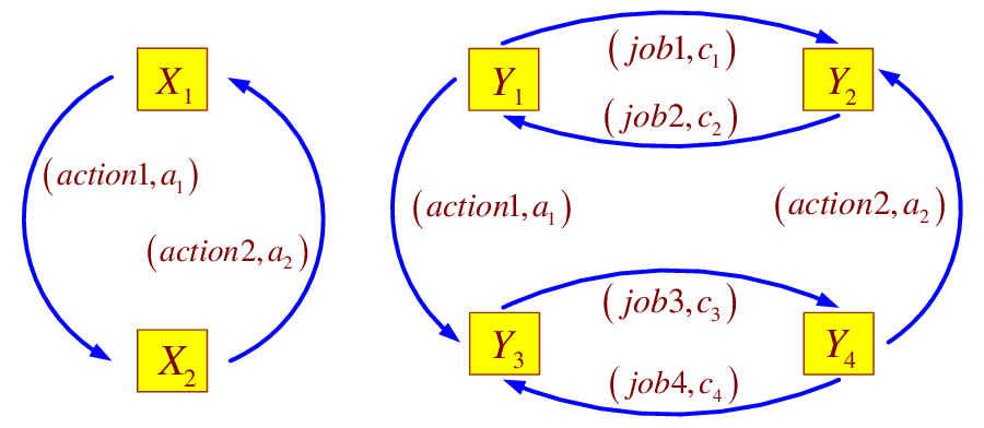
The operations of $X$ and $Y$ are illustrated in Figure 2. According to the mapping semantics, the derived ODEs from this model are

\left\{\begin{split}\frac{\mathrm{d}x_{1}}{\mathrm{d}t}&=-a_{1}\min\{x_{1},y_{1}\}+a_{2}\min\{x_{2},y_{4}\}\\ \frac{\mathrm{d}x_{2}}{\mathrm{d}t}&=a_{1}\min\{x_{1},y_{1}\}-a_{2}\min\{x_{2},y_{4}\}\\ \frac{\mathrm{d}y_{1}}{\mathrm{d}t}&=-a_{1}\min\{x_{1},y_{1}\}-c_{1}y_{1}+c_{2}y_{2}\\ \frac{\mathrm{d}y_{2}}{\mathrm{d}t}&=-c_{2}y_{2}+a_{2}\min\{x_{2},y_{4}\}+c_{1}y_{1}\\ \frac{\mathrm{d}y_{3}}{\mathrm{d}t}&=-c_{3}y_{3}+c_{4}y_{4}+a_{1}\min\{x_{1},y_{1}\}\\ \frac{\mathrm{d}y_{4}}{\mathrm{d}t}&=-a_{2}\min\{x_{2},y_{4}\}-c_{4}y_{4}+c_{3}y_{3}\end{split}\right.,

(53)

where $x_{i},y_{j}\;(i=1,2,\;j=1,2,\cdots,4)$ denote the populations of $X$ and $Y$ in the local derivatives $X_{i},Y_{j}$ respectively. Now we state an interesting assertion for the specific PEPA model: the difference between the number of $Y$ in their local derivatives $Y_{3}$ and $Y_{4}$ , and the number of $X$ in the local derivative $X_{2}$ , i.e. $y_{3}+y_{4}-x_{2}$ , is a constant in any state. This fact can be explained as follows. Notice that there is only one way to increase $y_{3}+y_{4}$ , i.e. enabling the activity $action1$ . As long as $action1$ is activated, then there is a copy of $Y$ entering the $Y_{3}$ from $Y_{1}$ . Meanwhile, since $action1$ is shared by $X$ , a corresponding copy of $X$ will go to $X_{2}$ from $X_{1}$ . In other words, $y_{3}+y_{4}$ and $x_{2}$ increase equally and simultaneously. On the other hand, there is also only one way to decrease $y_{3}+y_{4}$ and $x_{2}$ , i.e. enabling the cooperated activity $action2$ . This also allows $y_{3}+y_{4}$ and $x_{2}$ to decrease both equally and simultaneously. So, the difference $y_{3}+y_{4}-x_{2}$ will remain constant in any state and thus at any time. The assertion indicates that each state and therefore the whole state space of underlying CTMC may have some interesting structure properties, such as invariants. The techniques and applications of structural analysis of PEPA models have been developed in [22].

Throughout this section, let $M$ and $N$ be the total populations of the $X$ and $Y$ respectively, i.e. $M=M_{1}+M_{2}$ and $N=N_{1}+N_{2}+N_{3}+N_{4}$ . Notice $y_{1}+y_{2}+y_{3}+y_{4}=N$ and $x_{1}+x_{2}=M$ by the conservation law, so $y_{1}+y_{2}-x_{1}=N-M-(y_{3}+y_{4}-x_{2})$ is another invariant because $y_{3}+y_{4}-x_{2}$ is a constant. The fluid-approximation version of these two invariants also holds, which is illustrated by the following Lemma 6.

Lemma 6.

For any $t\geq 0$ ,

\begin{split}y_{1}(t)+y_{2}(t)-x_{1}(t)&=y_{1}(0)+y_{2}(0)-x_{1}(0),\\ y_{3}(t)+y_{4}(t)-x_{2}(t)&=y_{3}(0)+y_{4}(0)-x_{2}(0).\end{split}

Proof.

According to (53), for any $t\geq 0$ ,

\frac{\mathrm{d}(y_{1}(t)+y_{2}(t)-x_{1}(t))}{\mathrm{d}t}=\frac{\mathrm{d}y_{1}}{\mathrm{d}t}+\frac{\mathrm{d}y_{2}}{\mathrm{d}t}-\frac{\mathrm{d}x_{1}}{\mathrm{d}t}=0.

So $y_{1}(t)+y_{2}(t)-x_{1}(t)=y_{1}(0)+y_{2}(0)-x_{1}(0)$ , $\forall t\geq 0$ . By a similar argument, we also have $y_{3}(t)+y_{4}(t)-x_{2}(t)=y_{3}(0)+y_{4}(0)-x_{2}(0)$ , $\forall t\geq 0$ . ∎

In the following we show how to use this kind of invariance to prove the convergence of the solution of (53) as time goes to infinity. Before presenting the results and the proof, we first rewrite (53) as follows:

\begin{split}\left(\begin{array}[]{c}\frac{\mathrm{d}x_{1}}{\mathrm{d}t}\\ \frac{\mathrm{d}x_{2}}{\mathrm{d}t}\\ \frac{\mathrm{d}y_{1}}{\mathrm{d}t}\\ \frac{\mathrm{d}y_{2}}{\mathrm{d}dt}\\ \frac{\mathrm{d}y_{3}}{\mathrm{d}t}\\ \frac{\mathrm{d}y_{4}}{\mathrm{d}t}\end{array}\right)=&I_{\{x_{1}<y_{1},x_{2}<y_{4}\}}Q_{1}\left(\begin{array}[]{c}x_{1}\\ x_{2}\\ y_{1}\\ y_{2}\\ y_{3}\\ y_{4}\end{array}\right)+I_{\{x_{1}<y_{1},x_{2}\geq y_{4}\}}Q_{2}\left(\begin{array}[]{c}x_{1}\\ x_{2}\\ y_{1}\\ y_{2}\\ y_{3}\\ y_{4}\end{array}\right)\\ &+I_{\{x_{1}\geq y_{1},x_{2}<y_{4}\}}Q_{3}\left(\begin{array}[]{c}x_{1}\\ x_{2}\\ y_{1}\\ y_{2}\\ y_{3}\\ y_{4}\end{array}\right)+I_{\{x_{1}\geq y_{1},x_{2}\geq y_{4}\}}Q_{4}\left(\begin{array}[]{c}x_{1}\\ x_{2}\\ y_{1}\\ y_{2}\\ y_{3}\\ y_{4}\end{array}\right),\end{split}

(54)

where the matrices $Q_{i}\;(i=1,2,3,4)$ are given as below:

\displaystyle Q_{1}=\left(\begin{array}[]{cc|cccc}-a_{1}&a_{2}&&&&\\ a_{1}&-a_{2}&&&\\ \hline\cr-a_{1}&&-c_{1}&c_{2}&&\\ &a_{2}&c_{1}&-c_{2}&&\\ a_{1}&&&&-c_{3}&c_{4}\\ &-a_{2}&&&c_{3}&-c_{4}\end{array}\right),

\displaystyle Q_{2}=\left(\begin{array}[]{cc|cccc}-a_{1}&0&&&&a_{2}\\ a_{1}&0&&&&-a_{2}\\ \hline\cr-a_{1}&0&-c_{1}&c_{2}&&\\ &0&c_{1}&-c_{2}&&a_{2}\\ a_{1}&0&&&-c_{3}&c_{4}\\ &0&&&c_{3}&-(c_{4}+a_{2})\end{array}\right),

\displaystyle Q_{3}=\left(\begin{array}[]{cc|cccc}0&a_{2}&-a_{1}&&&\\ 0&-a_{2}&a_{1}&&&\\ \hline\cr 0&&-a_{1}-c_{1}&c_{2}&&\\ 0&a_{2}&c_{1}&-c_{2}&&\\ 0&&a_{1}&&-c_{3}&c_{4}\\ 0&-a_{2}&&&c_{3}&-c_{4}\end{array}\right),

\displaystyle Q_{4}=\left(\begin{array}[]{cc|cccc}0&0&-a_{1}&&&a_{2}\\ 0&0&a_{1}&&&-a_{2}\\ \hline\cr 0&0&-a_{1}-c_{1}&c_{2}&&\\ 0&0&c_{1}&-c_{2}&&a_{2}\\ 0&0&a_{1}&&-c_{3}&c_{4}\\ 0&0&&&c_{3}&-a_{2}-c_{4}\end{array}\right).

As (54) illustrates, the derived ODEs are piecewise linear and they may be dominated by $Q_{i}\;(i=1,2,3,4)$ alternately. If the system is always dominated by only one specific matrix after a time, then the ODEs become linear after this time. For linear ODEs, as long as the eigenvalues of their coefficient matrices are either zeros or have negative real parts, then bounded solutions will converge as time tends to infinity, see Corollary 3 in D. Fortunately, here the eigenvalues of the matrices $Q_{i}\;(i=1,2,3,4)$ in Model 2 satisfy this property, the proof of which is shown in C. In addition, the solution of the derived ODEs from any PEPA model is bounded, as Theorem 5 illustrated. Therefore, if we can guarantee that after a time the ODEs (54) become linear, which means that one of the four matrices $Q_{i}\;(i=1,2,3,4)$ will be the coefficient matrix of the linear ODEs, then by Corollary 3 the solution will converge. So the convergence problem is reduced to determining whether the linearity can be finally guaranteed.

It is easy to see that the comparisons between $x_{1}$ and $y_{1}$ , $x_{2}$ and $y_{4}$ determine the linearity. For instance, if after a time $T$ , we always have $x_{1}>y_{1}$ and $x_{2}>y_{4}$ , then the matrix $Q_{4}$ will dominate the system. Fortunately, the invariance in the model, as Lemma 6 reveals, can determine the comparisons in some circumstances. This is because this invariance reflects the relationship between different component types that are connected through synchronisations. This leads to several conclusions as follows.

Proposition 8.

If $y_{1}(0)+y_{2}(0)\leq x_{1}(0)$ and $y_{3}(0)+y_{4}(0)\leq x_{2}(0)$ , then the solution of (54) converges.

Proof.

By Lemma 6, $y_{1}(t)+y_{2}(t)\leq x_{1}(t)$ and $y_{3}(t)+y_{4}(t)\leq x_{2}(t)$ for all time $t$ . Since both $y_{2}(t)$ and $y_{4}(t)$ are nonnegative by Theorem 5, we have $y_{1}(t)\leq x_{1}(t)$ and $y_{4}(t)\leq x_{2}(t)$ for any $t$ . Thus, (54) becomes

\left(\frac{\mathrm{d}x_{1}}{\mathrm{d}t},\frac{\mathrm{d}x_{2}}{\mathrm{d}t},\frac{\mathrm{d}y_{1}}{\mathrm{d}t},\frac{\mathrm{d}y_{2}}{\mathrm{d}t},\frac{\mathrm{d}y_{3}}{\mathrm{d}t},\frac{\mathrm{d}y_{4}}{\mathrm{d}t}\right)^{T}=Q_{4}\left(x_{1},x_{2},y_{1},y_{2},y_{3},y_{4}\right)^{T}.

(59)

Notice that (59) is linear, and all eigenvalues of $Q_{4}$ other than zeros have negative real parts, then according to Corollary 3, the solution of (59) converges as time goes to infinity. ∎

Proposition 9.

Suppose $y_{1}(0)+y_{2}(0)>x_{1}(0)$ and $y_{3}(0)+y_{4}(0)\leq x_{2}(0)$ . If either (I). $\displaystyle N>\left(2+\frac{a_{1}+c_{1}}{c_{2}}\right)M$ , or (II). $\displaystyle N>\frac{2(c_{1}+c_{2})+a_{2}}{c_{2}}M$ , where $N>M>0$ are the populations of $Y$ and $X$ respectively, then the solution of (54) converges.

Proof.

Suppose (I) holds. According to the conservation law, $\sum_{i=1}^{4}y_{i}(t)=N$ . By the boundedness of the solution, we have $x_{2}(t)\leq M$ . Then by Lemma 6, $y_{3}(t)+y_{4}(t)\leq x_{2}(t)\leq M$ . Therefore,

y_{2}(t)=N-(y_{3}(t)+y_{4}(t))-y_{1}(t)\geq N-M-y_{1}(t).

(60)

Since $\min\{x_{1},y_{1}\}\leq y_{1}$ , so $-a\min\{x_{1},y_{1}\}\geq-a_{1}y_{1}$ . Thus

\begin{split}\frac{\mathrm{d}y_{1}}{\mathrm{d}t}&=-a_{1}\min\{x_{1},y_{1}\}-c_{1}y_{1}+c_{2}y_{2}\\ &\geq-a_{1}y_{1}-c_{1}y_{1}+c_{2}y_{2}\\ &\geq-(a_{1}+c_{1})y_{1}+c_{2}(N-M-y_{1})\\ &=-(a_{1}+c_{1}+c_{2})y_{1}+c_{2}(N-M).\end{split}

(61)

That is

\frac{\mathrm{d}y_{1}}{\mathrm{d}t}\geq-(a_{1}+c_{1}+c_{2})y_{1}+c_{2}(N-M).

Applying Lemma 14 in A to this formula, we have

y_{1}(t)\geq\left(y_{1}(0)-\frac{c_{2}(N-M)}{a_{1}+c_{1}+c_{2}}\right)e^{-(a_{1}+c_{1}+c_{2})t}+\frac{c_{2}(N-M)}{a_{1}+c_{1}+c_{2}}.

(62)

Since the first term of the right side of (62) converges to zero as time goes to infinity, i.e. $\displaystyle\lim_{t\rightarrow\mathchar 561\relax}\left(y_{1}(0)-\frac{c_{2}(N-M)}{a_{1}+c_{1}+c_{2}}\right)e^{-(a_{1}+c_{1}+c_{2})t}=0$ , and the second term $\displaystyle\frac{c_{2}(N-M)}{a_{1}+c_{1}+c_{2}}>M$ which results from the condition $\displaystyle N>\left(2+\frac{a_{1}+c_{1}}{c_{2}}\right)M$ , then there exists $T>0$ such that for any $t>T$ , $y_{1}(t)>M\geq x_{1}(t)$ . Then after time $T$ , (54) becomes linear, and is dominated by $Q_{2}$ . Because all eigenvalues of $Q_{2}$ are either zeros or have negative real parts, the solution converges as time goes to infinity.

Now we assume $(II)$ holds. Similarly, since $\min\{x_{2},y_{4}\}\leq x_{2}\leq M$ , and $y_{1}\leq N-y_{2}$ which is due to $y_{1}+y_{2}\leq N$ , we have

\begin{split}\frac{\mathrm{d}y_{2}}{\mathrm{d}t}&=-c_{2}y_{2}+a_{2}\min\{x_{2},y_{4}\}+c_{1}y_{1}\\ &\leq-c_{2}y_{2}+a_{2}M+c_{1}y_{1}\\ &\leq-c_{2}y_{2}+a_{2}M+c_{1}(N-y_{2})\\ &=-(c_{1}+c_{2})y_{2}+a_{2}M+c_{1}N.\end{split}

(63)

By Lemma 14 in A,

y_{2}\leq\left(y_{2}(0)-\frac{a_{2}M+c_{1}N}{c_{1}+c_{2}}\right)e^{-(c_{1}+c_{2})t}+\frac{a_{2}M+c_{1}N}{c_{1}+c_{2}}.

(64)

Therefore, since $e^{-(c_{1}+c_{2})t}$ in above formula converges to zero as time tends to infinity, then for any $\epsilon>0$ , there exists $T>0$ such that for any time $t>T$ ,

y_{2}\leq\frac{a_{2}M+c_{1}N}{c_{1}+c_{2}}+\epsilon.

(65)

Notice that the condition $\displaystyle N>\frac{2(c_{1}+c_{2})+a_{2}}{c_{2}}M$ implies

\displaystyle\frac{c_{2}N-a_{2}M-(c_{1}+c_{2})M}{c_{1}+c_{2}}>M,

and let $\epsilon$ be small enough that $\displaystyle\frac{c_{2}N-a_{2}M-(c_{1}+c_{2})M}{c_{1}+c_{2}}-\epsilon>M.$ Then by (60), $y_{1}\geq(N-M)-y_{2}$ . Therefore,

\begin{split}y_{1}&\geq(N-M)-y_{2}\\ &\geq(N-M)-\frac{a_{2}M+c_{1}N}{c_{1}+c_{2}}-\epsilon\\ &=\frac{c_{2}N-a_{2}M-(c_{1}+c_{2})M}{c_{1}+c_{2}}-\epsilon\\ &>M\geq x_{1}.\end{split}

(66)

So $y_{1}(t)>x_{1}(t)$ , $y_{4}(t)\leq x_{2}(t)$ , for any $t>T$ , then by a similar argument the solution of (54) converges. ∎

Both condition (I) and (II) in Proposition 9 require $N$ to be larger enough than $M$ , to guarantee that $y_{1}$ is larger than $x_{1}$ . Since our PEPA model is symmetric, Proposition 9 has a corresponding symmetric version.

Proposition 10.

Suppose $y_{1}(0)+y_{2}(0)\leq x_{1}(0)$ and $y_{3}(0)+y_{4}(0)>x_{2}(0)$ . If either (I). $\displaystyle N>\left(2+\frac{a_{2}+c_{3}}{c_{4}}\right)M$ , or (II). $\displaystyle N>\frac{2(c_{3}+c_{4})+a_{1}}{c_{1}}M$ , where $N>M>0$ are the populations of $Y$ and $X$ respectively, then the solution of (54) converges.

The proof of Proposition 10 is omitted here. We should point out that in our model the shared activity $action1$ (respectively, $action2$ ) has the same local rate $a_{1}$ (respectively, $a_{2}$ ). We have taken the advantage of this in the above proofs. If the local rates of shared activities are not set to be the same, analogous conclusions can still hold but the discussion will be more complicated. However, the structural property invariance can still play an important role.

The above three propositions have illustrated the convergence for all situations in terms of the starting state, except for the case of $y_{1}(0)+y_{2}(0)>x_{1}(0),y_{3}(0)+y_{4}(0)>x_{2}(0).$ See a summary in Table 3. If $y_{1}(0)+y_{2}(0)>x_{1}(0)$ , $y_{3}(0)+y_{4}(0)>x_{2}(0)$ , then the dynamic behaviour of the system is rather complex. A numerical study for this case will be presented in the next subsection.

Table 3: A summary for the convergence of Model 2

Starting state condition	Additional condition	Conclusion
$y_{1}(0)+y_{2}(0)\leq x_{1}(0)$ ,
$y_{3}(0)+y_{4}(0)\leq x_{2}(0)$	No	Proposition 8
$y_{1}(0)+y_{2}(0)>x_{1}(0)$ ,
$y_{3}(0)+y_{4}(0)\leq x_{2}(0)$	$N>k_{1}M$	Proposition 9
$y_{1}(0)+y_{2}(0)\leq x_{1}(0)$ ,
$y_{3}(0)+y_{4}(0)>x_{2}(0)$	$N>k_{2}M$	Proposition 10
$y_{1}(0)+y_{2}(0)>x_{1}(0)$ ,
$y_{3}(0)+y_{4}(0)>x_{2}(0)$	None identified	Explored numerically

6.2.2 Experimental study of convergence

This subsection presents a numerical study at different action rate conditions. The starting state in this subsection is always assumed as $(1,1,5,0,0,5)$ , which satisfies the condition of $y_{1}(0)+y_{2}(0)>x_{1}(0)$ and $y_{3}(0)+y_{4}(0)>x_{2}(0)$ .

If all the action rates in the model are set to one, i.e. $(a_{1},a_{2},c_{1},c_{2},c_{3},c_{4})=(1,1,1,1,1,1)$ , then the equilibrium point of the ODEs is $(x_{1}^{*},x_{2}^{*},y_{1}^{*},y_{2}^{*},y_{3}^{*},y_{4}^{*})=(1,1,2,3,3,2)$ , as the numerical solution of the ODEs illustrates. In this case, the matrix $Q_{1}$ finally dominates the system. See Figure 3. Notice that in this figure, the curves of $x_{1}$ and $x_{2}$ completely overlap, as well as the curves of $y_{1}$ and $y_{4}$ , and those of $y_{2}$ and $y_{3}$ .

In other situations, for example, if $(a_{1},a_{2},c_{1},c_{2},c_{3},c_{4})=(1,1,1,10,1,10)$ then the equilibrium point is $(0.4616,1.5384,4.0140,0.4476,5.0769,0.4615)$ , and the matrix $Q_{2}$ eventually dominates the system. See Figure 4. Moreover, the matrices $Q_{3}$ and $Q_{4}$ can also finally dominate the system as long as the action rates are appropriately specified. See Figure 5 and Figure 6. We should point out that similarly to Figure 3, in Figure 6 the curves of $x_{1}$ and $x_{2}$ , the curves of $y_{1}$ and $y_{4}$ , as well as those of $y_{2}$ and $y_{3}$ respectively, completely overlap.

In short, the system dynamics is rather complex in the situation of $y_{1}(0)+y_{2}(0)>x_{1}(0)$ and $y_{3}(0)+y_{4}(0)>x_{2}(0)$ . A summary of these numerical studies is organised in Table 4.

Table 4: Complex dynamical behaviour of Model 2: starting state (1,1,5,0,0,5)

Rates:	Equilibrium points:	Dominator	Figure
$(a_{1},a_{2},c_{1},c_{2},c_{3},c_{4})$	$(x_{1}^{},x_{2}^{},y_{1}^{},y_{2}^{},y_{3}^{},y_{4}^{})$
$(1,1,1,1,1,1)$	$(1,1,2,3,3,2)$	$Q_{1}$	Figure 3
$(1,1,1,10,1,10)$	$v_{1}$ ³³ 3 $v_{1}=(0.4616,1.5384,4.0140,0.4476,5.0769,0.4615)$	$Q_{2}$	Figure 4
$(1,1,10,1,1,1)$	$v_{2}$ ⁴⁴ 4 $v_{2}=(1.5384,0.4616,0.4615,5.0769,2.4616,2.0000)$	$Q_{3}$	Figure 5
$(20,20,1,1,1,1)$	$(1,1,0.2273,4.7727,4.7727,0.2273)$	$Q_{4}$	Figure 6

7 Fluid analysis: an analytic approach (II)

7.1 Convergence for two component types and one synchronisation (I): a special case

The problem of convergence for more general models without strict conditions, is rather complex and has not been completely solved. But for a particular class of PEPA model — a model composed of two types of component with one synchronisation between them, we can determine the convergence of the solutions of the derived ODEs.

As discussed in the previous section, the ODEs derived from PEPA are piecewise linear and may be dominated by different coefficient matrices alternately. For any PEPA model which has two component types and one synchronisation, the two corresponding coefficient matrices can be proved to have a good property: their eigenvalues are either zeros or have negative real parts. The remaining issue for convergence is to ascertain that these two matrices will not always alternately dominate the system. In fact, we will prove that under some mild conditions, there exists a time after which there is only one coefficient matrix dominating the system. This means the ODEs become linear after that time. Since the coefficient matrix of the linear ODEs satisfies the good eigenvalue property, then by Corollary 3, the bounded solution will converge as time goes to infinity.

We first utilise an example in this section to show our approach to dealing with the convergence problem for this class of PEPA models. The proof for a general case in this class is presented in the next subsection.

7.1.1 A previous model and the fluid approximation

Let us look at the following PEPA model, which is Model 1 presented previously:

\begin{split}User_{1}\stackrel{{\scriptstyle\mbox{{\tiny def}}}}{{=}}&(task_{1},a).User_{2}\\ User_{2}\stackrel{{\scriptstyle\mbox{{\tiny def}}}}{{=}}&(task_{2},b).User_{1}\\ Provider_{1}\stackrel{{\scriptstyle\mbox{{\tiny def}}}}{{=}}&(task_{1},a).Provider_{2}\\ Provider_{2}\stackrel{{\scriptstyle\mbox{{\tiny def}}}}{{=}}&(reset,d).Provider_{1}\\ (User_{1}[M])&\raisebox{-4.30554pt}{$\;\stackrel{{\scriptstyle\mbox{\large$\rhd\!\!\!\lhd$}}}{{\scriptscriptstyle\{task1\}}}\,$}(Provider_{1}[N]).\end{split}

The derived ODEs are as follows:

\left\{\begin{split}\frac{\mathrm{d}x_{1}}{\mathrm{d}t}&=-a\min\{x_{1},y_{1}\}+bx_{2}\\ \frac{\mathrm{d}x_{2}}{\mathrm{d}t}&=a\min\{x_{1},y_{1}\}-bx_{2}\\ \frac{\mathrm{d}y_{1}}{\mathrm{d}t}&=-a\min\{x_{1},y_{1}\}+dy_{2}\\ \frac{\mathrm{d}y_{2}}{\mathrm{d}t}&=a\min\{x_{1},y_{1}\}-dy_{2}\\ \end{split}\right.

(67)

where $x_{i}$ and $y_{i}$ represent the populations of $User_{i}$ and $Provider_{i}$ respectively, $i=1,2$ . Clearly, (67) is equivalent to

\left(\begin{array}[]{c}\frac{\mathrm{d}x_{1}}{\mathrm{d}t}\\ \frac{\mathrm{d}x_{2}}{\mathrm{d}t}\\ \frac{\mathrm{d}y_{1}}{\mathrm{d}t}\\ \frac{\mathrm{d}y_{2}}{\mathrm{d}t}\\ \end{array}\right)=I_{\{x_{1}\leq y_{1}\}}Q_{1}\left(\begin{array}[]{c}x_{1}\\ x_{2}\\ y_{1}\\ y_{2}\\ \end{array}\right)+I_{\{x_{1}>y_{1}\}}Q_{2}\left(\begin{array}[]{c}x_{1}\\ x_{2}\\ y_{1}\\ y_{2}\\ \end{array}\right),

(68)

where

Q_{1}=\left(\begin{array}[]{cc|cc}-a&b&0&0\\ a&-b&0&0\\ \hline\cr-a&0&0&d\\ a&0&0&-d\end{array}\right),\quad Q_{2}=\left(\begin{array}[]{cc|cc}0&b&-a&0\\ 0&-b&a&0\\ \hline\cr 0&0&-a&d\\ 0&0&a&-d\end{array}\right).

(69)

Our interest is to see if the solution of (68) will converge as time goes to infinity. As we mentioned, this convergence problem can be divided into two subproblems, i.e. whether the nonlinear equations can finally become linear and whether the eigenvalues of the coefficient matrix are either zeros or have negative real parts. If answers to these two subproblems are both positive, then the convergence will hold.

The second subproblem can be easily dealt with. By calculations, the matrix $Q_{1}$ has eigenvalues $0$ (two folds), $-d$ , and $-(a+b)$ . Similarly, $Q_{2}$ has eigenvalues $0$ (two folds), $-b,-(a+d)$ . Therefore, the eigenvalues of $Q_{1}$ and $Q_{2}$ other than zeros are negative. Moreover, for a general PEPA model which has two component types and one synchronisation, Theorem 7 in the next section shows that the corresponding coefficient matrices always have this property.

The remaining work to determine the convergence of the ODE solution, is to solve the first subproblem, i.e. to ascertain that after a time it is always the case that $x_{1}>y_{1}$ or $x_{1}\leq y_{1}$ . In this model, there is no invariance relating the two different component types, so we cannot rely on invariants to investigate this subproblem. However, we have a new way to cope with this problem.

7.1.2 Proof outline of convergence

Notice that $y_{1}(t)\leq N$ by the boundedness of solutions. If we can prove that after time $T$ , $x_{1}(t)\geq cM$ , where $c>0$ is independent of $M$ , we will get, provided $cM>N$ ,

x_{1}(t)\geq cM>N\geq y_{1}(t),\;t\geq T.

Therefore, the ODEs (67) will become linear after time $T$ . In the following, we identify that $x_{1}(t)\geq cM$ .

Let

\alpha(t)=\left\{\begin{array}[]{cc}\frac{\min\{x_{1}(t),y_{1}(t)\}}{x_{1}(t)},&x_{1}(t)\neq 0,\\ 1,&x_{1}(t)=0,\end{array}\right.

then $0\leq\alpha(t)\leq 1$ by the nonnegativity of $x_{1}(t)$ and $y_{1}(t)$ . The ODEs associated with component type $X$ can be rewritten as

\left\{\begin{split}\frac{\mathrm{d}x_{1}}{\mathrm{d}t}&=-a\alpha(t)x_{1}+bx_{2},\\ \frac{\mathrm{d}x_{2}}{\mathrm{d}t}&=a\alpha(t)x_{1}-bx_{2}.\end{split}\right.

(70)

Let

A(t)=\left(\begin{array}[]{cc}-a\alpha(t)&b\\ a\alpha(t)&-b\\ \end{array}\right),\quad X(t)=\left(\begin{array}[]{c}x_{1}(t)\\ x_{2}(t)\end{array}\right).

Then (70) can be written as

\frac{dX(t)}{dt}=A(t)X(t).

(71)

The solution of (71) is

\displaystyle{X(t)=e^{\int_{0}^{t}A(s)ds}X(0)}.

(72)

Let $\displaystyle B(t)=\frac{1}{t}\int_{0}^{t}A(s)ds$ , then

X(t)=e^{\int_{0}^{t}A(s)ds}X(0)=e^{tB(t)}X(0),

(73)

and

\begin{split}B(t)&=\frac{1}{t}\left(\begin{array}[]{cc}-a\int_{0}^{t}\alpha(s)ds&bt\\ a\int_{0}^{t}\alpha(s)ds&-bt\\ \end{array}\right)=\left(\begin{array}[]{cc}-a\beta(t)&b\\ a\beta(t)&-b\\ \end{array}\right),\end{split}

(74)

where $\displaystyle\beta(t)=\frac{\int_{0}^{t}\alpha(s)ds}{t}$ . Obviously, $0\leq\beta(t)\leq 1$ because $0\leq\alpha(s)\leq 1$ . Notice that the matrix $B(t)$ can be diagonalised as

\begin{split}B(t)&=\left(\begin{array}[]{cc}-a\beta(t)&b\\ a\beta(t)&-b\\ \end{array}\right)\\ &=\left(\begin{array}[]{cc}\frac{b}{a\beta(t)+b}&1\\ \frac{a\beta(t)}{a\beta(t)+b}&-1\\ \end{array}\right)\left(\begin{array}[]{cc}0&0\\ 0&-(a\beta(t)+b)\\ \end{array}\right)\left(\begin{array}[]{cc}1&1\\ \frac{a\beta(t)}{a\beta(t)+b}&-\frac{b}{a\beta(t)+b}\\ \end{array}\right)\\ &=U(t)\left(\begin{array}[]{cc}0&0\\ 0&-(a\beta(t)+b)\\ \end{array}\right)U^{-1}(t),\end{split}

(75)

where

U(t)=\left(\begin{array}[]{cc}\frac{b}{a\beta(t)+b}&1\\ \frac{a\beta(t)}{a\beta(t)+b}&-1\\ \end{array}\right),\quad U^{-1}(t)=\left(\begin{array}[]{cc}1&1\\ \frac{a\beta(t)}{a\beta(t)+b}&-\frac{b}{a\beta(t)+b}\\ \end{array}\right),

(76)

X(t)=e^{tB(t)}X(0)=U(t)\left(\begin{array}[]{cc}1&0\\ 0&e^{-t(a\beta(t)+b)}\\ \end{array}\right)U^{-1}(t)X(0).

(77)

In the formula (75), both $0$ and $-(a\beta(t)+b)$ are $B(t)$ ’s eigenvalues, while the columns of $U(t)$ are the corresponding eigenvectors. In particular, $\displaystyle\left(\frac{b}{a\beta(t)+b},\frac{a\beta(t)}{a\beta(t)+b}\right)^{T}$ , i.e. the first column of $U(t)$ , is the eigenvector corresponding to the eigenvalue zero.

We define a function $\hat{X}(t)$ by

\hat{X}(t)=U(t)\left(\begin{array}[]{cc}1&0\\ 0&0\\ \end{array}\right)U^{-1}(t)X(0).

(78)

By simple calculation,

\displaystyle\hat{X}(t)=(\hat{x}_{1}(t),\hat{x}_{2}(t))^{T}=\left(\frac{bM}{a\beta(t)+b},\frac{a\beta(t)M}{a\beta(t)+b}\right)^{T}.

(79)

Clearly, $\hat{X}(t)$ is the normalised eigenvector corresponding the zero eigenvalue (at the time $t$ ). Here the normalisaton is in terms of the total population $M$ of the component type $X$ . Moreover, $\hat{X}(t)$ embodies some equilibrium meaning. In fact, we have a conclusion:

\lim_{t\rightarrow\mathchar 561\relax}\|X(t)-\hat{X}(t)\|=0.

(80)

Since the explicit expression of $U(t)$ is available, the proof of (80) is easy and thus omitted. This conclusion is also included in Proposition 12, the proof of which does not rely on the explicit information of $U(t)$ and will be introduced later.

Now we discuss the benefit brought by this formula. By (80) the first entry of $X(t)$ approximates the first entry of $\hat{X}(t)$ , i.e. $x_{1}(t)$ approximates $\displaystyle\hat{x}_{1}(t)=\frac{bM}{a\beta(t)+b}$ . Thus, for any $\epsilon>0$ , there exists $T>0$ such that for any $t\geq T$ ,

x_{1}(t)>\hat{x}_{1}(t)-\epsilon=\frac{bM}{a\beta(t)+b}-\epsilon.

Since $\displaystyle\frac{bM}{a+b}\leq\frac{bM}{a\beta(t)+b}\leq M$ because $0\leq\beta(t)\leq 1$ , so $\displaystyle x_{1}(t)>\frac{bM}{a+b}-\epsilon$ . Therefore, if $\displaystyle\frac{bM}{a+b}>N$ , then by the boundedness of $y_{1}(t)$ , i.e. $y_{1}(t)\leq N$ , we have

x_{1}(t)>\frac{bM}{a+b}-\epsilon>N\geq y_{1}(t),

as long as $\epsilon$ is small enough. This means that $Q_{2}$ will dominate the system after time $T$ . So we have

Proposition 11.

If $\displaystyle\frac{bM}{a+b}>N$ , then the solution of the ODEs (68) converges as time tends to infinity.

Since the model is symmetric, this proposition has a symmetric version: if $\displaystyle\frac{dN}{a+d}>M$ , then the solution of the ODEs also converges.

As we discussed, there are two key steps in the proof of Proposition 11. The first step is to establish the approximation of $x_{1}(t)$ to $\hat{x}_{1}(t)$ , i.e. $x_{1}(t)\approx\hat{x}_{1}(t)$ . The second one is to give an estimation $\hat{x}_{1}(t)\geq cM$ . According to these two conclusions, we have $x_{1}(t)\geq c^{\prime}M$ where $c^{\prime}<c$ , and therefore can conclude that $x_{1}(t)\geq c^{\prime}M>N>y_{1}(t)$ provided the condition $c^{\prime}M>N$ . This is the main philosophy behind our proof for $x_{1}(t)>y_{1}(t)$ .

For the sake of generality, the proofs of these two conclusions should not rely on the explicit expressions of the eigenvalues and eigenvectors of $B(t)$ . This is because for general PEPA models with two component types and one synchronisation, these explicit expressions are not always available. The following subsection will present our discussions about these steps, and the proofs for the conclusions which do not rely on these explicit expressions.

7.1.3 Proof not relying on explicit expressions

This subsection will divide into two parts. In the first part, we will give a lower bound for the eigenvalues of the coefficient matrix $B(t)$ , based on which a proof of the approximation of $X(t)$ to $\hat{X}(t)$ is given. The second part will establish the estimation $\hat{x}_{1}(t)\geq cM$ . All proofs in this subsection do not require knowledge of the explicit expressions of the eigenvalues and eigenvectors of $B(t)$ .

For convenience, in this subsection we define

f(\beta)=\left(\begin{array}[]{cc}-a\beta&b\\ a\beta&-b\\ \end{array}\right),

(81)

where $f$ is a matrix-valued function defined on $\mathbb{R}$ . Then the matrix

\begin{split}B(t)=\left(\begin{array}[]{cc}-a\beta(t)&b\\ a\beta(t)&-b\\ \end{array}\right)\end{split}

can be written as $B(t)=f(\beta(t))$ . The diagonalisation of $f(\beta)$ is

\begin{split}f(\beta)=g(\beta)\left(\begin{array}[]{cc}0&0\\ 0&\lambda(\beta)\\ \end{array}\right)g^{-1}(\beta),\end{split}

where $\lambda(\beta)$ is $f(\beta)$ ’s nonzero eigenvalue, and $g(\beta)$ is a matrix whose columns are the eigenvectors of $f(\beta)$ . Here $g^{-1}(\beta)$ is the inverse of the matrix $g(\beta)$ . Notice that $\lambda(\beta)$ is real, because if $\lambda(\beta)$ is complex then its conjugation must be an eigenvalue, which is contradicted by the fact that $f(\beta)$ only has two eigenvalues, $0$ and $\lambda(\beta)$ . The following discussions in this subsection do not rely on the explicit expressions of $\lambda(\beta)$ , $g(\beta)$ and $g^{-1}(\beta)$ , although it is easy to see that $\lambda(\beta)=-a\beta+b$ and

g(\beta)=\left(\begin{array}[]{cc}\frac{b}{a\beta+b}&1\\ \frac{a\beta}{a\beta+b}&-1\\ \end{array}\right),\quad g^{-1}(\beta)=\left(\begin{array}[]{cc}1&1\\ \frac{a\beta}{a\beta+b}&-\frac{b}{a\beta+b}\\ \end{array}\right).

1. $X(t)$ approximates $\hat{X}(t)$

In the following, we will give a lower bound for the nonzero eigenvalue of $f(\beta)$ , i.e. $\lambda(\beta)$ , and based on this prove the approximation of $A(t)$ to $\hat{X}(t)$ as time tends to infinity.

If $\beta>0$ , then the transpose of $f(\beta)$ , i.e. $f(\beta)^{T}$ , is an infinitesimal generator, and thus the nonzero eigenvalue $\lambda(\beta)$ has negative real part, i.e. $\Re(\lambda(\beta))<0$ . If $\beta=0$ , then $f(\beta)$ is independent of $\beta$ and becomes a nonnegative matrix, i.e. each entry of it is nonnegative. Based on the Perron-Frobenious theorem which is presented in the next subsection, we can still have $\Re(\lambda(0))<0$ . Therefore, for any $\beta$ , $f(\beta)$ ’s eigenvalue other than zero has negative real part. This conclusion is stated in the following lemma.

Lemma 7.

For any $\beta\in[0,1]$ , $\Re(\lambda(\beta))<0$ , where $\lambda(\beta)$ is a nonzero eigenvalue of $f(\beta)$ .

The proof of Lemma 7 is presented in D.3. Lemma 7 can further lead to the following

Lemma 8.

Let

\Lambda_{1}=\inf_{\beta\in[0,1]}\{-\Re(\lambda(\beta))\mid\lambda(\beta)\;\mbox{is $f(\beta)$'s non-zero eigenvalue}\},

(82)

then $\Lambda_{1}>0$ .

Proof.

By Lemma 7, $-\Re(\lambda(\beta))>0$ for any $\beta\in[0,1]$ , so $\Lambda_{1}\geq 0$ . Suppose $\Lambda_{1}=0$ . Because the eigenvalue $\lambda(\beta)$ is a continuous function of the matrix $f(\beta)$ , where $f(\beta)$ is also continuous on $[0,1]$ with respect to $\beta$ , so $\lambda(\beta)$ is a continuous function of $\beta$ on $[0,1]$ . This is due to the fact that a composition of continuous functions is still continuous. Noticing $\Re(\cdot)$ is also a continuous function, so $-\Re(\lambda(\beta))$ is continuous with respect to $\lambda(\beta)$ , and thus with respect to $\beta$ on $[0,1]$ . Since a continuous function on a closed interval can achieve its minimum, there exists $\beta_{0}\in[0,1]$ such that $-\Re(\lambda(\beta_{0}))$ achieves the minimum $\Lambda_{1}$ , i.e. $-\Re(\lambda(\beta_{0}))=\Lambda_{1}=0$ . This is contradicted to Lemma 7. Therefore, $\Lambda_{1}>0$ . ∎

For any $t\in[0,\mathchar 561\relax)$ , $\beta(t)\in[0,1]$ . Noticing $B(t)=f(\beta(t))$ , therefore

\begin{split}&\{\lambda\mid\lambda\;\mbox{is $B(t)$'s non-zero eigenvalue},t>0\}\\ =&\{\lambda\mid\lambda\;\mbox{is $f(\beta(t))$'s non-zero eigenvalue},t>0\}\\ \subseteq&\{\lambda\mid\lambda\;\mbox{is $f(\beta)$'s non-zero eigenvalue};\beta\in[0,1]\}.\end{split}

(83)

Thus,

\begin{split}\Lambda&\triangleq\inf\{-\Re(\lambda)\mid\lambda\;\mbox{is $B(t)$'s nonzero eigenvalue},t>0\}\\ &\geq\inf\{-\Re(\lambda)\mid\lambda\;\mbox{is $f(\beta)$'s non-zero eigenvalue};\beta\in[0,1]\}=\Lambda_{1}.\end{split}

(84)

Because $\Lambda_{1}>0$ by Lemma 8, so $\Lambda>0$ . That is,

Corollary 1.

Let

\Lambda=\inf_{t\geq 0}\{-\Re(\lambda(t))\mid\lambda(t)\;\mbox{is $B(t)$'s non-zero eigenvalue}\},

then $\Lambda>0$ .

Based on this corollary, we can prove the approximation of $X(t)$ to $\hat{X}(t)$ .

Proposition 12.

Let $X(t)=(x_{1}(t),x_{2}(t))^{T}=e^{tB(t)}X(0)$ , i.e. the solution of (70). Let $\hat{X}(t)$ be defined by (78), i.e.

\hat{X}(t)=\left(\begin{array}[]{c}\hat{x}_{1}(t)\\ \hat{x}_{2}(t)\\ \end{array}\right)=U(t)\left(\begin{array}[]{cc}1&\\ &0\\ \end{array}\right)U(t)^{-1}\left(\begin{array}[]{c}x_{1}(0)\\ x_{2}(0)\\ \end{array}\right).

(85)

Then $\displaystyle\lim_{t\rightarrow\mathchar 561\relax}\|X(t)-\hat{X}(t)\|=0$ .

Proof.

Notice that eigenvectors of a matrix are continuous functions of the matrix. Since $g(\beta)$ is composed of the eigenvectors of the matrix $f(\beta)$ and $f(\beta)$ is continuous on $[0,1]$ with respect to $\beta$ , therefore $g(\beta)$ is continuous on $[0,1]$ with respect to $\beta$ . Because the inverse of a matrix is a continuous mapping, so $g^{-1}(\beta)$ , i.e. the inverse of $g(\beta)$ , is continuous with respect to $g(\beta)$ , and therefore is continuous on $[0,1]$ with respect to $\beta$ since $g(\beta)$ is continuous on $[0,1]$ . Since any continuous function is bounded on a compact set $[0,1]$ , both $g(\beta)$ and $g^{-1}(\beta)$ are bounded on $[0,1]$ . That is, there exists $K>0$ such that $\|g(\beta)\|\leq K$ and $\|g^{-1}(\beta)\|\leq K$ for all $\beta\in[0,1]$ . Because

\{U(t)\mid t\in[0,\mathchar 561\relax)\}=\{g(\beta(t))\mid t\in[0,\mathchar 561\relax)\}\subseteq\{g(\beta)\mid\beta\in[0,1]\},

we have

\displaystyle\sup_{t\geq 0}\|U(t)\|\leq\sup_{\beta\in[0,1]}\|g(\beta)\|\leq K.

Similarly, $\displaystyle\sup_{t\geq 0}\left\|U^{-1}(t)\right\|\leq K$ . Notice

\begin{split}X(t)-\hat{X}(t)=&e^{tB(t)}X(0)-U(t)\left(\begin{array}[]{cc}1&0\\ 0&0\\ \end{array}\right)U(t)^{-1}X(0)\\ =&\left[U(t)\left(\begin{array}[]{cc}1&0\\ 0&e^{t\lambda(t)}\\ \end{array}\right)U(t)^{-1}-U(t)\left(\begin{array}[]{cc}1&0\\ 0&0\\ \end{array}\right)U(t)^{-1}\right]X(0)\\ =&U(t)\left(\begin{array}[]{cc}0&0\\ 0&e^{t\lambda(t)}\\ \end{array}\right)U(t)^{-1}X(0),\end{split}

where $\lambda(t)$ is $B(t)$ ’s nonzero eigenvalue. By a similar argument to $\lambda(\beta)$ , $\lambda(t)$ is also real. Therefore,

-\lambda(t)=\Re(-\lambda(t))=-\Re(\lambda(t))\geq\Lambda>0

or $\lambda(t)\leq-\Lambda<0$ , where $\Lambda$ is defined in Corollary 1. Then

\begin{split}\|X(t)-\hat{X}(t)\|=&\left\|U(t)\left(\begin{array}[]{cc}0&0\\ 0&e^{t\lambda(t)}\\ \end{array}\right)U(t)^{-1}X(0)\right\|\\ \leq&\|U(t)\|\left\|\left(\begin{array}[]{cc}0&0\\ 0&e^{t\lambda(t)}\\ \end{array}\right)\right\|\|U(t)^{-1}\|\|X(0)\|\\ \leq&K^{2}\|X(0)\|e^{t\lambda(t)}\\ \leq&K^{2}\|X(0)\|e^{-t\Lambda}.\end{split}

Here we have used the norm property: $\|AB\|\leq\|A\|\|B\|$ . Since $\Lambda>0$ , we have $\displaystyle\lim_{t\rightarrow\mathchar 561\relax}\|X(t)-\hat{X}(t)\|=0$ . ∎

2: An lower-bound estimation on population in local derivatives

In the following, we will prove that there exists $T$ , such that $\hat{x}_{1}(t)\geq cM$ for any $t>T$ . We first define a function

h(\beta)=(h_{1}(\beta),h_{2}(\beta))^{T}=g(\beta)\left(\begin{array}[]{cc}1&0\\ 0&0\\ \end{array}\right)g^{-1}(\beta)\left(\begin{array}[]{c}x_{1}(0)\\ x_{2}(0)\\ \end{array}\right).

Clearly, we have $\hat{X}(t)=h(\beta(t))$ and $\hat{x}_{1}(t)=h_{1}(\beta(t))$ . Since $\beta(t)\in[0,1]$ for all $t$ , the following proposition can imply $\hat{x}_{1}(t)\geq cM$ .

Proposition 13.

There exists $c>0$ such that

\inf_{\beta\in[0,1]}h_{1}(\beta)\geq cM.

where $M=x_{1}(0)+x_{2}(0)$ , $c$ is independent of $M$ .

Proof.

Without loss of generality, we assume $M=1$ . We will show $\displaystyle\inf_{\beta\in[0,1]}h_{1}(\beta)=c>0$ . Since $h_{1}(\beta)$ is a continuous function of $\beta$ which is due to the continuity of $g(\beta)$ and $g^{-1}(\beta)$ , $h_{1}(\beta)$ can achieve its minimum on $[0,1]$ . That is, there exists $\beta_{0}\in[0,1]$ , such that

h_{1}(\beta_{0})=\inf_{\beta\in[0,1]}h_{1}(\beta)=c.

Consider the matrix

f(\beta_{0})=\left(\begin{array}[]{cc}-a\beta_{0}&b\\ a\beta_{0}&-b\\ \end{array}\right)

and a set of linear ODEs

\left(\begin{array}[]{c}\frac{\mathrm{d}z_{1}}{\mathrm{d}t}\\ \frac{\mathrm{d}z_{2}}{\mathrm{d}t}\\ \end{array}\right)=f(\beta_{0})\left(\begin{array}[]{c}z_{1}\\ z_{2}\\ \end{array}\right).

(86)

The solution of (86), given an initial value $Z(0)=X(0)=(x_{1}(0),x_{2}(0))^{T}$ , is $Z(t)=e^{tf(\beta_{0})}X(0)$ .

According to (75), $f(\beta_{0})$ can be diagonalised as

f(\beta_{0})=g(\beta_{0})\left(\begin{array}[]{cc}0&0\\ 0&\lambda(\beta_{0})\\ \end{array}\right)g^{-1}(\beta_{0}).

where $\lambda(\beta_{0})$ is the nonzero and real eigenvalue of $f(\beta_{0})$ . Thus

\begin{split}Z(t)=e^{tf(\beta_{0})}X(0)&=g(\beta_{0})\left(\begin{array}[]{cc}1&0\\ 0&e^{t\lambda(\beta_{0})}\\ \end{array}\right)g(\beta_{0})^{-1}\left(\begin{array}[]{c}x_{1}(0)\\ x_{2}(0)\\ \end{array}\right).\end{split}

(87)

Because $\lambda(\beta_{0})<0$ by Lemma 7, so as time goes to infinity,

\begin{split}Z(t)&=g(\beta_{0})\left(\begin{array}[]{cc}1&0\\ 0&e^{t\lambda(\beta_{0})}\\ \end{array}\right)g(\beta_{0})^{-1}\left(\begin{array}[]{c}x_{1}(0)\\ x_{2}(0)\\ \end{array}\right)\\ &\longrightarrow g(\beta_{0})\left(\begin{array}[]{cc}1&0\\ 0&0\\ \end{array}\right)g(\beta_{0})^{-1}\left(\begin{array}[]{c}x_{1}(0)\\ x_{2}(0)\\ \end{array}\right)=h(\beta_{0}).\end{split}

(88)

That is, $\displaystyle\lim_{t\rightarrow\mathchar 561\relax}Z(t)=h(\beta_{0})$ . In the following, we discuss two possible cases: $\beta_{0}>0$ and $\beta_{0}=0$ .

If $\beta_{0}>0$ , then the transpose of the matrix $f(\beta_{0})$ , i.e. $f(\beta_{0})^{T}$ , is an infinitesimal generator of an irreducible CTMC, which has two states and the transition rates between these two states are $a\beta_{0}$ and $b$ respectively. Moreover, the transient distribution of this CTMC, denoted by $Z(t)=(z_{1}(t),z_{2}(t))^{T}$ , satisfies the ODEs (86). As time goes to infinity, the transient distribution $Z(t)$ converges to the unique steady-state probability distribution. Since $\displaystyle\lim_{t\rightarrow\mathchar 561\relax}Z(t)=h(\beta_{0})$ , therefore $h(\beta_{0})=(h_{1}(\beta_{0}),h_{2}(\beta_{0}))^{T}$ is the steady-state probability distribution and thus $h_{1}(\beta_{0})>0$ . So $\inf_{\beta\in[0,1]}h_{1}(\beta)=h_{1}(\beta_{0})>0$ .

If $\beta_{0}=0$ , then

f(\beta_{0})=\left(\begin{array}[]{cc}0&b\\ 0&-b\\ \end{array}\right).

Since $\displaystyle\lim_{t\rightarrow\mathchar 561\relax}Z(t)=h(\beta_{0})$ , therefore $\displaystyle\left(\frac{\mathrm{d}z_{1}}{\mathrm{d}t},\frac{\mathrm{d}z_{2}}{\mathrm{d}t}\right)^{T}$ converges to zero. Letting time go to infinity on the both sides of (86), we obtain the following equilibrium equations,

\left(\begin{array}[]{c}0\\ 0\\ \end{array}\right)=f(\beta_{0})\left(\begin{array}[]{c}h_{1}(\beta_{0})\\ h_{2}(\beta_{0})\\ \end{array}\right).

(89)

By the conservation law, $(h_{1}(\beta_{0})+h_{2}(\beta_{0}))^{T}=M=1$ . Therefore, $(h_{1}(\beta_{0}),h_{2}(\beta_{0}))^{T}$ satisfies

\left\{\begin{array}[]{c}f(\beta_{0})(h_{1}(\beta_{0}),h_{2}(\beta_{0}))^{T}=0,\\ h_{1}(\beta_{0})+h_{2}(\beta_{0})=M=1.\end{array}\right.

(90)

Solving (90), we obtain the unique solution $(h_{1}(\beta_{0}),h_{2}(\beta_{0}))^{T}=(1,0)^{T}$ . Therefore, $h_{1}(\beta_{0})$ is one, and thus $\inf_{\beta\in[0,1]}h_{1}(\beta)=h_{1}(\beta_{0})>0$ . ∎

Remark 4.

As $\beta$ tends to $0$ ,

f(\beta)=\left(\begin{array}[]{cc}-a\beta&b\\ a\beta&-b\\ \end{array}\right)\longrightarrow f(0)=\left(\begin{array}[]{cc}0&b\\ 0&-b\\ \end{array}\right).

Correspondingly, for the equilibrium $h(\beta)=(h_{1}(\beta),h_{2}(\beta))^{T}=\left(\frac{bM}{a\beta+b},\frac{a\beta M}{a\beta+b}\right)^{T}$ satisfying $f(\beta)h(\beta)=0$ and $h_{1}(\beta)+h_{2}(\beta)=M$ , we have $\left(\frac{bM}{a\beta+b},\frac{a\beta M}{a\beta+b}\right)^{T}\rightarrow(M,0)^{T}$ as $\beta$ tends to zero. From the explicit expression, i.e. $h_{1}(\beta)=\frac{bM}{a\beta+b}$ , the minimum and maximum of $h_{1}(\beta)$ are $\frac{bM}{a+b}$ and $M$ respectively, which correspond to the matrices $f(1)$ and $f(0)$ respectively. In the context of the PEPA model, $f(1)$ corresponds to a free subsystem and there is no synchronisation effect on it, i.e. the subsystem of component type $X$ is independent of $Y$ . The matrix $f(0)$ reflects that the subsystem of $X$ has been influenced by the subsystem of $Y$ , i.e. the rates of shared activities are determined by $Y$ , that is, the term $a\min\{x_{1},y_{1}\}$ has been replaced by $ay_{1}$ . Therefore the exit rates from the local derivative $X_{1}$ correspondingly become smaller since now $ay_{1}<ax_{1}$ . In order to balance the flux, which is described by the equilibrium equation, the population of $X_{1}$ must increase. That is why the equilibrium $h_{1}(\beta)$ increases as $\beta$ decreases. In short, synchronisations can increase the populations in syncrhonised local derivatives in the steady state.

As an application of the above facts, if $h_{1}(\beta_{0})>0$ for some $\beta_{0}>0$ , then we can claim that $h_{1}(0)>0$ because $h_{1}(0)\geq h_{1}(\beta_{0})>0$ .

Obviously, Proposition 13 has a corollary:

Corollary 2.

There exists $c>0$ such that for any $t\in[0,\mathchar 561\relax)$ , $\hat{x}_{1}(t)\geq cM.$

Proposition 12 and Proposition 13 can lead to the following lemma.

Lemma 9.

There exists $c>0,T>0$ , such that $x_{1}(t)\geq cM$ for all $t\geq T$ .

Proof.

By Proposition 13 or Corollary 2, there exists $c_{1},T_{1}>0$ such that $\hat{x}_{1}(t)\geq c_{1}M$ for any $t>T_{1}$ . By Proposition 12, $\lim_{t\rightarrow\mathchar 561\relax}|x_{1}(t)-\hat{x}_{1}(t)|=0$ , which implies that for any $\epsilon$ , there exists $T_{2}>0$ such that for any $t>T_{2}$ , $x_{1}(t)>\hat{x}_{1}(t)-\epsilon$ . Choose $T_{2}>T_{1}$ , then we have

x_{1}(t)>\hat{x}_{1}(t)-\epsilon\geq c_{1}M-\epsilon.

Therefore, there exist $c,T>0$ such that such that $x_{1}(t)\geq cM$ for all $t>T$ . ∎

Because $x_{1}(t)\geq cM$ , provided $cM>N$ we have $x_{1}(t)\geq cM>N\geq y_{1}(t)$ , i.e., the system will finally become linear. In the following we will show how to apply our method to more general cases.

7.2 Convergence for two component types and one synchronisation (II): general case

This section deals with such an arbitrary PEPA model which has two component types and one synchronisation. The local action rates of the shared activity are not assumed to be the same. The main result of this section is a convergence theorem: as long as the population of one component type is sufficiently larger than the population of the other, then the solution of the derived ODEs converges as time tends to infinity.

7.2.1 Features of coefficient matrix

We assume the component types to be $X$ and $Y$ . The component type $X$ is assumed to have local derivatives $X_{1},X_{2},\cdots,X_{m}$ , while $Y$ has local derivatives $Y_{1},Y_{2},\cdots,Y_{n}$ . We use $x_{i}(t)$ to denote the population of $X$ in $X_{i}\;(i=1,\cdots,m)$ at time $t$ . Similarly, $y_{j}(t)$ denotes the population of $Y$ in $Y_{j}\;(j=1,\cdots,n)$ at time $t$ . Without loss of generality, we assume the synchronisation is associated with the local derivatives $X_{1}$ and $Y_{1}$ , i.e. the nonlinear term in the derived ODEs is $\min\{rx_{1}(t),sy_{1}(t)\}$ where $r$ and $s$ are some constants. In fact, if the synchronisation is associated with $X_{i}$ and $Y_{j}$ , by appropriately permuting their suffixes, i.e. $i\rightarrow 1,\;i+1\rightarrow 2,\;\cdots\;,i-1\rightarrow m$ , $j\rightarrow 1,\;j+1\rightarrow 2,\;\cdots\;,j-1\rightarrow n$ , the synchronisation will be associated with $X_{1}$ and $Y_{1}$ . According to the mapping semantics presented previously, the derived ODEs from this class of PEPA model are

\begin{split}\frac{\mathrm{d}\mathbf{x}}{\mathrm{d}t}=\sum_{l}lf(\mathbf{x},l)\end{split}

(91)

where $\mathbf{x}=(x_{1}(t),\cdots,x_{m}(t),y_{1}(t),\cdots,y_{n}(t))^{T}$ . For convenience, we denote

X(t)=\left(x_{1}(t),x_{2}(t),\cdots,x_{m}(t)\right)^{T},

Y(t)=\left(y_{1}(t),y_{2}(t),\cdots,y_{n}(t)\right)^{T}.

In (91) all terms are linear except for those containing “ $\min\{rx_{1}(t),sy_{1}(t)\}$ ”. Notice

\min\{rx_{1}(t),sy_{1}(t)\}=I_{\{rx_{1}(t)\leq sy_{1}(t)\}}rx_{1}(t)+I_{\{rx_{1}(t)>sy_{1}(t)\}}sy_{1}(t).

When $rx_{1}(t)\leq sy_{1}(t)$ , which is indicated by $I_{\{rx_{1}(t)\leq sy_{1}(t)\}}=1$ and $I_{\{rx_{1}(t)>sy_{1}(t)\}}=0$ , we can replace $\min\{rx_{1}(t),sy_{1}(t)\}$ by $rx_{1}(t)$ in (91). Then (91) becomes linear since all nonlinear terms are replaced by linear terms $rx_{1}(t)$ , so the ODEs have the following form,

\left(\begin{array}[]{c}\frac{\mathrm{d}X}{\mathrm{d}t}\\ \frac{\mathrm{d}Y}{\mathrm{d}t}\\ \end{array}\right)=Q_{1}\left(\begin{array}[]{c}X\\ Y\\ \end{array}\right),

(92)

where $Q_{1}$ is a coefficient matrix. Similarly, if $rx_{1}(t)>sy_{1}(t)$ , $\min\{rx_{1}(t),sy_{1}(t)\}$ can be replaced by $sy_{1}(t)$ in (91). Then (91) can become

\left(\begin{array}[]{c}\frac{\mathrm{d}X}{\mathrm{d}t}\\ \frac{\mathrm{d}Y}{\mathrm{d}t}\\ \end{array}\right)=Q_{2}\left(\begin{array}[]{c}X\\ Y\\ \end{array}\right),

(93)

where $Q_{2}$ is another coefficient matrix corresponding to the case of $rx_{1}(t)>sy_{1}(t)$ .

In short, the derived ODEs (91) are just the following

\left(\begin{array}[]{c}\frac{\mathrm{d}X}{\mathrm{d}t}\\ \frac{\mathrm{d}Y}{\mathrm{d}t}\\ \end{array}\right)=I_{\{rx_{1}\leq sy_{1}\}}Q_{1}\left(\begin{array}[]{c}X\\ Y\\ \end{array}\right)+I_{\{rx_{1}>sy_{1}\}}Q_{2}\left(\begin{array}[]{c}X\\ Y\\ \end{array}\right).

(94)

The case discussed in the previous section is a special case of this kind of form. If the conditions $rx_{1}(t)\leq sy_{1}(t)$ and $rx_{1}(t)>sy_{1}(t)$ occur alternately, then the matrices $Q_{1}$ and $Q_{2}$ will correspondingly alternately dominate the system, as Figure 7 illustrates.

Similar to the cases discussed in the previous two sections, the convergence problem of (94) can be divided into two subproblems, i.e. to examine whether the following two properties hold:

1.

There exists a time $T$ , such that either $x_{1}\leq y_{1},\;\forall t>T$ or $x_{1}\leq y_{1},\;\forall t>T$ .
2.

The eigenvalues of $Q_{1}$ and $Q_{2}$ other than zeros have negative real parts.

The first item can guarantee (94) to eventually have a constant linear form, while the second item ensures the convergence of the bounded solution of the linear ODEs. If the answers to these two problems are both positive, then the convergence of the solution of (94) will hold. The study of these two problems are discussed in the next two subsections. In the remainder of this subsection, we first investigate the structure property of the coefficient matrices $Q_{1}$ and $Q_{2}$ in (94).

The structure of the coefficient matrices $Q_{1}$ and $Q_{2}$ is determined by the following two propositions, which indicate that they are either block lower-triangular or block upper-triangular.

Proposition 14.

$Q_{1}$ in (94) can be written as

Q_{1}=\left(\begin{array}[]{cc}\hat{Q}_{1}&0\\ W&V_{n\times n}\\ \end{array}\right)_{(m+n)\times(m+n)},

(95)

where $\hat{Q}_{1}^{T}$ is an infinitesimal generator matrix with the dimension ${m\times m}$ , and

W_{n\times m}=\left(\begin{array}[]{cccc}w_{11}&0&\cdots&0\\ w_{21}&0&\cdots&0\\ \vdots&\vdots&\vdots&\vdots\\ w_{n1}&0&\cdots&0\end{array}\right),

(96)

where $w_{11}<0$ , $w_{j1}(j=2,\cdots,n)\geq 0$ and $\sum_{j=1}^{n}w_{j1}=0$ . Here $V$ and $W$ satisfy that if we let

P=\left(W_{1}+V_{1},V_{2},\cdots,V_{n}\right),

(97)

i.e. $P$ ’s first column is the sum of $V$ ’s first column and $W$ ’s first column, while $P$ ’s other columns are the same to $V$ ’s other columns, then $P^{T}$ is also an infinitesimal generator matrix.

Proof.

Let

Q_{1}=\left(\begin{array}[]{cc}\hat{Q}_{1}&U\\ W&V\end{array}\right),

(98)

where $\hat{Q}_{1}$ and $V$ are $m\times m$ and $n\times n$ matrices respectively. Suppose $rx_{1}(t)\leq sy_{1}(t)$ , then

\begin{split}\left(\begin{array}[]{c}\frac{\mathrm{d}X}{\mathrm{d}t}\\ \frac{\mathrm{d}Y}{\mathrm{d}t}\\ \end{array}\right)=Q_{1}\left(\begin{array}[]{c}X\\ Y\\ \end{array}\right)=\left(\begin{array}[]{cc}\hat{Q}_{1}&U\\ W&V\end{array}\right)\left(\begin{array}[]{c}X\\ Y\\ \end{array}\right).\end{split}

(99)

So we have

\frac{\mathrm{d}X}{\mathrm{d}t}=\hat{Q}_{1}X+UY.

(100)

The condition $rx_{1}(t)\leq sy_{1}(t)$ implies that all nonlinear terms $\min\{rx_{1}(t),sy_{1}(t)\}$ can be replaced by $x_{1}(t)$ . This means that the behaviour of the component type $X$ in (99) and (100) is independent of the component type $Y$ . Thus in (99) $U$ must be a zero matrix, i.e.

Q_{1}=\left(\begin{array}[]{cc}\hat{Q}_{1}&0\\ W&V\end{array}\right).

Moreover, (100) becomes

\frac{\mathrm{d}X}{\mathrm{d}t}=\hat{Q}_{1}X,

(101)

that is, there is no synchronisation in the ODEs corresponding to the component type $X$ given $rx_{1}(t)\leq sy_{1}(t)$ . Then by Proposition 4, $\hat{Q}_{1}^{T}$ is an infinitesimal generator.

According to (99),

\begin{split}\frac{\mathrm{d}Y}{\mathrm{d}t}&=WX+VY\\ &=(W_{1},W_{2},\cdots,W_{m})(x_{1},x_{2},\cdots,x_{m})^{T}+VY\\ &=x_{1}W_{1}+VY+\sum_{i=2}^{m}x_{i}W_{i},\end{split}

(102)

where $W=(W_{1},W_{2},\cdots,W_{m})$ . Notice that the component type $Y$ is synchronised with the component type $X$ only through the term $\min\{rx_{1}(t),sy_{1}(t)\}=x_{1}(t)$ . In other words, in (102) $Y$ is directly dependent on only $x_{1}$ other than $x_{i}\;(i\geq 2)$ . This implies $W_{1}\neq 0$ while $W_{i}=0\;(i=2,3,\cdots,m)$ . Therefore,

\begin{split}\frac{\mathrm{d}Y}{\mathrm{d}t}&=x_{1}W_{1}+VY=x_{1}W_{1}+\sum_{j=1}^{n}y_{j}V_{j},\end{split}

(103)

where $V_{j}\;(j=1,2,\cdots,n)$ are the columns of $V$ . Denote $W_{1}=(w_{11},w_{21},\cdots,w_{n1})^{T}$ . Notice that $Y_{1}$ is a pre local derivative of the shared activity, and $x_{1}w_{11}$ represents the exit rates of the shared activity from $Y_{1}$ . Therefore, $w_{11}<0$ . Moreover, $x_{1}w_{j1}$ $(j=2,\cdots,n)$ are the synchronised entry rates for the local derivatives $Y_{j}\;(j=2,\cdots,n)$ respectively, so $w_{j1}\geq 0\;(j=2,\cdots,n)$ . By the conservation law, the total synchronised exit rates are equal to the total synchronised entry rates, i.e. $x_{1}\sum_{j=1}^{n}w_{j1}=0$ or $\sum_{j=1}^{n}w_{j1}=0$ .

We have known that $x_{1}$ in (103) derives from the synchronised term $\min\{rx_{1},sy_{1}\}$ . If the effect of the synchronisation on the behaviour of $Y$ is removed, i.e. recover $y_{1}$ by replacing $x_{1}$ , then (103) will become

\begin{split}\frac{\mathrm{d}Y}{\mathrm{d}t}&=y_{1}W_{1}+VY=y_{1}W_{1}+\sum_{j=1}^{n}y_{j}V_{j}=PY,\end{split}

(104)

where $P=(W_{1}+V_{1},V_{2},\cdots,V_{n})$ . Since there is no synchronisation contained in the subsystem of the component type $Y$ , according to Proposition 4, $P^{T}$ is the infinitesimal generator. ∎

Similarly, we can prove

Proposition 15.

$Q_{2}$ in (94) can be written as

Q_{2}=\left(\begin{array}[]{cc}E_{m\times m}&F\\ 0&\hat{Q}_{2}\\ \end{array}\right)_{(m+n)\times(m+n)},

(105)

where $\hat{Q}_{2}^{T}$ is an infinitesimal generator matrix with the dimension ${n\times n}$ , and

F_{m\times n}=\left(\begin{array}[]{cccc}f_{11}&0&\cdots&0\\ f_{21}&0&\cdots&0\\ \vdots&\vdots&\vdots&\vdots\\ f_{m1}&0&\cdots&0\end{array}\right),

(106)

where $f_{11}<0$ , $f_{j1}(j=2,\cdots,m)\geq 0$ and $\sum_{j=1}^{m}f_{j1}=0$ . Here $F$ and $E$ satisfy that if we let

R=\left(F_{1}+E_{1},E_{2},\cdots,E_{n}\right),

(107)

then $R^{T}$ is also an infinitesimal generator matrix.

7.2.2 Eigenvalues of coefficient matrix

In this subsection, we will determine the eigenvalue property of $Q_{1}$ and $Q_{2}$ . First, the Perron-Frobenius theorem gives an estimation of eigenvalues for nonnegative matrices.

Theorem 6.

(Perron-Frobenius). Let $A=(a_{ij})$ be a real $n\times n$ matrix with nonnegative entries $a_{ij}\geq 0$ . Then the following statements hold:

1.

There is a real eigenvalue $r$ of $A$ such that any other eigenvalue $\lambda$ satisfies $|\lambda|\leq r$ .
2.

$r$ satisfies $\min\limits_{i}\sum_{j}a_{ij}\leq r\leq\max\limits_{i}\sum_{j}a_{ij}$ .

Remark 5.

We should point out that in the second property, exchanging $i$ and $j$ in $a_{ij}$ in the formula, we still have $\min\limits_{i}\sum_{j}a_{ji}\leq r\leq\max\limits_{i}\sum_{j}a_{ji}$ . In fact, $A^{T}$ is also a real matrix with non-negative entries. Since $A^{T}$ and $A$ share the same eigenvalues, so $r$ is one of the eigenvalues of $A^{T}$ , such that any other eigenvalue $\lambda$ of $A^{T}$ satisfies $|\lambda|\leq r$ . Notice $(A^{T})_{ij}=A_{ji}$ , By applying the Perron-Frobenius theorem to $A^{T}$ , we have

\min\limits_{i}\sum_{j}a_{ji}\leq r\leq\max\limits_{i}\sum_{j}a_{ji}.

We cannot directly apply this theorem to our coefficient matrices $Q_{1}$ and $Q_{2}$ , since both of them have negative elements, not only on the diagonal but also in other entries. However, we use some well-known techniques in linear algebra, i.e. the following Lemma 10 and 11 (which can be easily found in linear algebra textbooks), to cope with this problem, and thus derive estimates of their eigenvalues.

Lemma 10.

If $E_{m\times m}$ and $F_{n\times n}$ have eigenvalues $\lambda_{i}\;(i=1,2,\cdots,m)$ and $\delta_{j}$ $(j=1,2,\cdots,n)$ respectively, then each of

H_{1}=\left(\begin{array}[]{cc}E&0\\ G&F\\ \end{array}\right),\;H_{2}=\left(\begin{array}[]{cc}E&G\\ 0&F\\ \end{array}\right)

has eigenvalues $\lambda_{i}\;(i=1,2,\cdots,m)$ and $\delta_{j}\;(j=1,2,\cdots,n)$ .

Lemma 11.

If $\lambda$ is an eigenvalue of $V$ , then $\lambda+r$ is an eigenvalue of $V+rI$ , where $r$ is a scalar.

Theorem 7.

The eigenvalues of both $Q_{1}$ and $Q_{2}$ are either zeros or have negative real parts.

Proof.

We only give the proof for $Q_{1}$ ’s case. By Proposition 14,

Q_{1}=\left(\begin{array}[]{cc}\hat{Q}_{1}&0\\ W&V_{n\times n}\\ \end{array}\right)_{(m+n)\times(m+n)}.

(108)

According to Lemma 10, if all eigenvalues of $\hat{Q}_{1}$ and $V$ are determined, then the eigenvalues of $Q_{1}$ will be determined. Let us consider $V$ first.

Notice that only diagonal elements of $V$ are possibly negative (which can be deduced from Proposition 14). Let $r=\sup\limits_{i}|V_{ii}|>0$ , then all the entries of $V+rI$ are nonnegative. Let $\lambda$ be an arbitrary eigenvalue of $V$ , then by Lemma 11, $\lambda+r$ is an eigenvalue of $V+rI$ .

Notice the sum of the elements of any column of $V$ is zero (because the sum of entry rates equals to the sum of exit rates), so $V$ has a zero eigenvalue with the corresponding eigenvector $\mathbf{1}$ , i.e. $V\mathbf{1}=\mathbf{0}$ . Thus $r=0+r$ is an eigenvalue of $V+rI$ . Moreover,

\min\limits_{i}\sum_{j}(V+rI)_{ji}=r=\max\limits_{i}\sum_{j}(V+rI)_{ji}.

Applying the Perron-Frobenius theorem (Theorem 6) and Remark 5 to $V+rI$ , so

|\lambda+r|\leq r.

(109)

Let $\lambda=a+bi$ , then (109) implies that $a\leq 0$ , and if $a=0$ then $b=0$ . In other words, $V$ ’s eigenvalues are either zeros or have negative real parts.

Similarly, $\hat{Q}_{1}$ ’s eigenvalues other than zeros have negative real parts. By Lemma 10, the eigenvalues of $Q_{1}$ other than zeros have negative real parts. The proof is complete. ∎

7.2.3 Convergence theorem

Now we deal with another subproblem: whether or not after a long time, we always have $rx_{1}\geq sy_{1}$ (or $rx_{1}<sy_{1}$ ). If the population of $X$ is significantly larger than the population of $Y$ , intuitively, there will finally be a greater number of $X$ in the local derivative $X_{1}$ , than the number of $Y$ in $Y_{1}$ . This will lead to $rx_{1}>sy_{1}$ .

Lemma 12.

Under the assumptions in Section 7.1.1, for the following ODEs

\left(\begin{array}[]{c}\frac{\mathrm{d}X}{\mathrm{d}t}\\ \frac{\mathrm{d}Y}{\mathrm{d}t}\\ \end{array}\right)=I_{\{rx_{1}\leq sy_{1}\}}Q_{1}\left(\begin{array}[]{c}X\\ Y\\ \end{array}\right)+I_{\{rx_{1}>sy_{1}\}}Q_{2}\left(\begin{array}[]{c}X\\ Y\\ \end{array}\right),

there exists $c_{1}>0,c_{2}>0,T>0$ , such that $x_{1}(t)\geq c_{1}M$ , $y_{1}(t)\geq c_{2}N$ for any $t\geq T$ , where $c_{1}$ and $c_{2}$ are independent of $M$ and $N$ .

Proof.

The proof is essentially the same as the proof of Lemma 9. We only give the sketch of the proof for $x_{1}(t)\geq c_{1}M$ . By introducing new two functions $\alpha(t)$ and $\beta(t)$ ,

\alpha(t)=\left\{\begin{array}[]{cc}\frac{\min\{rx_{1}(t),sy_{1}(t)\}}{rx_{1}(t)},&x_{1}(t)\neq 0,\\ 1,&x_{1}(t)=0,\end{array}\right.

\beta(t)=\frac{1}{t}\int_{0}^{t}\alpha(s)ds,

the nonlinear term $\min\{rx_{1}(t),sy_{1}(t)\}$ equals $r\alpha(t)x_{1}(t)$ , and thus the ODEs associated with the subsystem $X$ can be written as

\frac{\mathrm{d}X}{\mathrm{d}t}=A(t)X

(110)

where $A(t)$ is related to $\alpha(t)$ . The solution of (110) is $X(t)=e^{tB(t)}X(0)$ , where $B(t)$ is defined by $\displaystyle B(t)=\frac{1}{t}\int_{0}^{t}A(s)ds$ , and thus $B(t)$ is related to $\beta(t)$ .

Notice that according to Theorem 7 and its proof, the eigenvalues of $B(t)$ other than zeros have negative real parts for any $t>0$ . By a similar proof to Corollary 1, we have

\Lambda=\inf_{t\geq 0}\{-\Re(\lambda)\mid\lambda\;\mbox{is $B(t)$'s non-zero eigenvalue}\}>0.

(111)

This fact will lead to the conclusion that $X(t)$ can be approximated by $\hat{X}(t)$ , where $\hat{X}(t)$ is constructed similarly to the one in Proposition 12. Because a general $B(t)$ considered here may not be diagonalisable, so the construction of $\hat{X}(t)$ is a little bit more complicated. We detail the construction as well as the proof of the following result in D:

\lim_{t\rightarrow\mathchar 561\relax}\|X(t)-\hat{X}(t)\|=0.

Then, by similar arguments to Proposition 13 and Corollary 2, we can prove that $\inf_{t>T}\hat{x}_{1}(t)\geq cM$ , where $\hat{x}_{1}(t)$ is the first entry of $\hat{X}(t)$ . Then, by a similar proof to the proof of Lemma 9, we can conclude that there exists a number $c_{1}$ such that $x_{1}(t)\geq c_{1}M$ after a time $T$ . ∎

Lemma 13.

Under the assumptions of Lemma 12, if $M>K_{1}N$ or $N>K_{2}M$ , where constants $K_{1}>0$ and $K_{2}>0$ are sufficiently large, then there exists $T$ such that $rx_{1}(t)\geq sy_{1}(t),\;\forall t\geq T$ or $rx_{1}(t)\leq sy_{1}(t),\;\forall t\geq T$ respectively.

Proof.

By the boundedness of solutions, $0\leq x_{1}(t)\leq M$ and $0\leq y_{1}(t)\leq N$ for any $t$ . Suppose $M>K_{1}N$ . By Lemma 12, there exists $c,T>0$ , $x_{1}(t)\geq cM,\;\forall t\geq T$ . Since $K_{1}$ is assumed to be large enough such that $K_{1}\geq\frac{s}{rc}$ , then $rcM>sN$ . So for any $t>T$ , we have

rx_{1}(t)\geq rcM\geq sN\geq sy_{1}(t).

If $N>K_{2}M$ , the proof is similar and omitted here. ∎

Now we state our convergence theorem.

Theorem 8.

If $M>K_{1}N$ or $N>K_{2}M$ , where constants $K_{1},K_{2}>0$ are sufficiently large, then the solution of the derived ODEs (94), i.e.

\left(\begin{array}[]{c}\frac{\mathrm{d}X}{\mathrm{d}t}\\ \frac{\mathrm{d}Y}{\mathrm{d}t}\\ \end{array}\right)=I_{\{rx_{1}\leq sy_{1}\}}Q_{1}\left(\begin{array}[]{c}X\\ Y\\ \end{array}\right)+I_{\{rx_{1}>sy_{1}\}}Q_{2}\left(\begin{array}[]{c}X\\ Y\\ \end{array}\right),

converges to a finite limit as time goes to infinity.

Proof.

Suppose $M>K_{1}N$ , then by Lemma 13, there exists a time $T>0$ , such that after time $T$ , $rx_{1}(t)\geq sy_{1}(t)$ , so (94) becomes

\left(\begin{array}[]{c}\frac{\mathrm{d}X}{\mathrm{d}t}\\ \frac{\mathrm{d}Y}{\mathrm{d}t}\\ \end{array}\right)=Q_{2}\left(\begin{array}[]{c}X\\ Y\\ \end{array}\right).

(112)

Since $Q_{2}$ ’s eigenvalues other than zeros have strict negative real parts according to Theorem 7, and the solution of the above equation is bounded, then by Corollary 3, the solution converges to a finite limit as time goes to infinity. ∎

Remark 6.

We should point out that for a general PEPA model with two component types and one synchronisation, the limit of the solution of the derived ODEs is determined by the populations of these two component types rather than the particular starting state. That is to say, whatever the initial state is, as long as the total populations of the components are the same, the limit that the solution converges to will always be the same. We do not plan to discuss this topic in detail in this paper.

8 Related work

As we have mentioned in the introduction section, the fluid approximation approach was first proposed by Hillston in [21] to deal with the state space explosion problem in the context of PEPA. An interpretation as well as a justification of this approximation approach has been demonstrated by Hayden in his dissertation [33]. In [33, 34], generation of similar systems of coupled ODEs for higher-order moments such as variance has been addressed. Additionally, the dissertation [33] discusses how to derive stochastic differential equations from PEPA models.

More recently, some extensions of the previous mapping from PEPA to ODEs have been presented by Bradley et al. in [23]. In particular, passive rates are introduced into the fluid approximation. In the recent paper [35], different existing styles of passive cooperation in fluid models are compared and intensively discussed. Moreover, a new passive fluid semantics for passive cooperation, which can be viewed as approximating the first moments of the component counting processes, has been provided, with a theoretical justification. The paper [36] considers the application of this fluid approximation approach with modifications in the context of epidemiology. In this paper, the notions of side and self-loops are added to the activity matrix, and the rates are calculated differently, for the purpose of deriving from PEPA models the most commonly used ODEs in the context of epidemiology. In [37] and [38] by Tribastone, a new operational semantics is proposed to give a compact symbolic representation of PEPA models. This semantics extends the application scope of the fluid approximation of PEPA by incorporating all the operators of the language and removing earlier assumptions on the syntactical structure of the models amenable to this analysis.

The fluid approximation approach has also been applied to timed Petri nets to deal with the state space explosion problem [39, 40]. The comparison between the fluid approximation of PEPA models and timed continuous Petri nets has been demonstrated by Galpin in [41]. This paper has established links between two continuous approaches to modelling the performance of systems. In the paper, a translation from PEPA models to continuous Petri nets and vice versa has been presented. In addition, it has been shown that the continuous approximation using PEPA has infinite server semantics. The fluid approximation approach has also been used by Thomas to derive asymptotic solutions for a class of closed queueing networks [42]. In this paper, an analytical solution to a class of models, specified using PEPA, is derived through the ODE approach. It is shown that “this solution is identical to that used for many years as an asymptotic solution to the mean value analysis of closed queueing networks”.

Moreover, the relationship between the fluid approximation and the underlying CTMCs for a special PEPA model has been revealed by Geisweiller et al. in [25]: the ODEs derived from the PEPA description are the limits of the sequence of underlying CTMCs. It has been shown in [28] by Gilmore that for some special examples the equilibrium points of the ODEs derived from PEPA models coincide the steady-state probability distributions of the CTMCs underlying the nonsynchronised PEPA models.

In addition, there are several papers which discuss how to derive response time from the fluid approximation of PEPA models. In [43], by constructing an absorption operator for the PEPA language, Bradley et al. allow general PEPA models to be analysed for fluid-generated response times. Clark et al. demonstrate in [44] how to derive expected passage response times using Little’s law based on averaged populations of entities in an equilibrium state. This technique has been generalised into one for obtaining a full response-time profile computing the probability of a component observing the completion of a response at a given time after the initiation of the request, see [45]. Moreover, an error in the passage specification in the approach taken in [43] has been uncovered and rectified in [45] by Clark. The ODE method associated with the PEPA language has demonstrated successful application in the performance analysis of large scale systems [46, 47, 48, 49, 50].

9 Conclusions

In this paper, we have demonstrated how to derive the fluid approximation from a general PEPA model via the numerical representation of the PEPA language, which extended the current mapping semantics of fluid approximations. The fundamental properties of the fluid approximation such as the existence and uniqueness, boundedness and nonnegativeness of the solutions of the derived ODEs have been established. Moreover, the convergence of the solution under a particular condition for general models has been verified. This particular condition relates some famous constants of Markov chains such as the spectral gap and the Log-Sobolev constant. For the models without synchronisations or with one synchronisation and two component types, we have determined the convergence. Furthermore, the consistency between the fluid approximation and the CTMC in the context of PEPA has been revealed. If a model has no synchronisations, then the derived ODEs are just the probability distribution evolution equations of the underlying CTMC except for a scaling factor. For any general PEPA model, the ODEs can be taken as the corresponding density dependent CTMC with the concentration level infinity. In addition, the coefficient matrices of some derived ODEs were studied: their eigenvalues are either zeros or have negative real parts. The structural property of invariance has been shown to play an important role in the proof of convergence for some PEPA models. Due to the limitation of pages, we have not shown how to derive performance measurers from the fluid approximation, and have not given the numerical comparison between the fluid approximation and the CTMC in terms of performance measures. For more details, please refer to [22].

In addition to the established results, this paper has also demonstrated comprehensive techniques and methods to investigate the PEPA language: not only both theoretical and experimental, probabilistic and analytic, but also syntactic and numerical (investigating the models based on the numerical representation of PEPA), qualitative and quantitative (exploiting the structural property to verify the convergence). These results and techniques are expected to have more applications in performance modelling and evaluation of large scale systems.

Acknowledgements

Partial work of the first author was carried out in LFCS, School of Informatics and IDCom, School of Engineering, The University of Edinburgh, when he was a PhD student and supported by the Mobile VCE (www.mobilevce.com) Programme 4.

References

[1] J. Hillston, A Compositional Approach to Performance Modelling (PhD Thesis), Cambridge University Press, 1996.
[2] N. Götz, U. Herzog, M. Rettelbach, TIPP– a language for timed processes and performance evaluation, Tech. rep., Tech. Rep.4/92, IMMD7, University of Erlangen-Nörnberg, Germany (Nov. 1992).
[3] M. Bernardo, R. Gorrieri, A tutorial on EMPA: A theory of concurrent processes with nondeterminism, priorities, probabilities and time, Theoretical Computer Science 202 (1998) 1–54.
[4] H. Hermanns, Interactive Markov chains, Ph.D. thesis, Universität Erlangen-Nürnberg, Germany (1998).
[5] M. Sereno, Towards a product form solution for stochastic process algebras, The Computer Journal 38 (7) (1995) 622–632.
[6] J. Hillston, N. Thomas, Product form solution for a class of PEPA models, Performance Evaluation 35 (3–4) (1999) 171–192.
[7] G. Clark, J. Hillston, Product form solution for an insensitive stochastic process algebra structure, Performance Evaluation 50 (2–3) (2002) 129–151.
[8] P. G. Harrison, Turning back time in Markovian process algebra, Theor. Comput. Sci. 290 (3) (2003) 1947–1986.
[9] V. Mertsiotakis, Approximate analysis methods for stochastic process algebras, Ph.D. thesis, Universität Erlangen-Nürnberg, Erlangen (1998).
[10] H. C. Bohnenkamp, B. R. Haverkort, Semi-numerical solution of stochastic process algebra models, in: ARTS ’99: Proceedings of the 5th International AMAST Workshop on Formal Methods for Real-Time and Probabilistic Systems, Springer-Verlag, London, UK, 1999, pp. 228–243.
[11] J. Hillston, L. Kloul, An efficient Kronecker representation for PEPA models, in: PAPM-PROBMIV ’01: Proceedings of the Joint International Workshop on Process Algebra and Probabilistic Methods, Performance Modeling and Verification, Springer-Verlag, London, UK, 2001, pp. 120–135.
[12] J. Hillston, L. Kloul, Formal techniques for performance analysis: blending SAN and PEPA, Formal Aspects of Computing 19 (2007) 3–33.
[13] B. Buchholz, Compositional analysis of a Markovian process algebra, in: M. Rettelbach, U. Herzog (Eds.), Proc. of 2nd Process Algebra and Performance Modelling Workshop, 1994.
[14] M. Rettelbach, M. Siegle, Compositional minimal semantics for the stochastic process algebra TIPP, in: Proc. of 2nd Process Algebra and Performance Modelling Workshop, 1994, p. pages.
[15] M. J. A. Smith, Abstraction and model checking in the Eclipse PEPA plug-in, in: PASTA ’09: Proceedings of the 8th Workshop on Process Algebra and Stochastically Timed Acitvities, 2009.
[16] M. J. A. Smith, Compositional Abstraction of PEPA Models, http://lanther.co.uk/papers/PEPA_abstraction.pdf (2009).
[17] C. Priami, A. Regev, E. Shapiro, W. Silverman, Application of a stochastic name-passing calculus to representation and simulation of molecular processes, Inf. Process. Lett. 80 (1) (2001) 25–31.
[18] C. Kuttler, J. Niehren, Gene regulation in the $\pi$ -calculus: Simulating cooperativity at the lambda switch, Vol. 4230 of Lecture Notes in Computer Science, Springer Berlin / Heidelberg, 2006, pp. 24–55.
[19] M. Calder, A. Duguid, S. Gilmore, J. Hillston, Stronger computational modelling of signalling pathways using both continuous and discrete-state methods, in: Computational Methods in Systems Biology, Vol. 4210 of LNCS, Springer-Verlag, 2006, pp. 63–77.
[20] M. Calder, S. Gilmore, J. Hillston, Modelling the influence of RKIP on the ERK signalling pathway using the stochastic process algebra PEPA, in: Transactions on Computational Systems Biology VII, no. 4230 in LNCS, Springer, 2006.
[21] J. Hillston, Fluid flow approximation of PEPA models, in: International Conference on the Quantitative Evaluation of Systems (QEST’05), IEEE Computer Society, 2005.
[22] J. Ding, Structural and fluid analysis of large scale PEPA models — with applications to content adaptation systems, Ph.D. thesis, The Univeristy of Edinburgh (2010).
[23] J. T. Bradley, S. T. Gilmore, J. Hillston, Analysing distributed internet worm attacks using continuous state-space approximation of process algebra models, Journal of Computer and System Sciences 74 (6) (2008) 1013–1032.
[24] S. Gilmore, J. Hillston, M. Ribaudo, An efficient algorithm for aggregating PEPA models, IEEE Trans. Softw. Eng. 27 (5) (2001) 449–464.
[25] N. Geisweiller, J. Hillston, M. Stenico, Relating continuous and discrete PEPA models of signalling pathways, Theoretical Computer Science 404 (1-2) (2008) 97–111.
[26] G. Bolch, S. Greiner, H. d. Meer, K. S. Trivedi, Queueing Networks and Markov Chains: Modelling and Performance Evaluation with Computer Science Application, John Wiley & Sons, INC., 1998.
[27] J. H. Hubbard, B. H. West, Differential Equations: A Dynamical Systems Approach (Higher-Dimensional Systems), no. 18 in Texts in Applied Mathematics, Springer, 1990.
[28] S. Gilmore, Continuous-time and continuous-space process algebra, in: Process Algebra and Stochastically Timed Activities (PASTA’05), 2005.
[29] T. G. Kurtz, Solutions of ordinary differential equations as limits of pure jump Markov processes, Journal of Applied Probability 7 (1) (1970) 49–58.
[30] S. N. Ethier, T. G. Kurtz, Markov Processes: Characterization and Convergence, John Wiley & Sons, Inc., 1986.
[31] Z. Brzeźniak, T. Zastawniak, Basic Stochastic Processes, Springer Undergraduate Mathematics Series, Springer, 1999.
[32] L. Saloff-Coste, Lectures on finite Markov chains, in: Lecture Notes in Mathematics, Vol. 1665, Springer, Berlin, 1997.
[33] R. Hayden, Addressing the state space explosion problem for PEPA models through fluid-flow approximation, http://pubs.doc.ic.ac.uk/fluid-spa-modelling/ (July 2007).
[34] R. A. Hayden, J. T. Bradley, ODE-based general moment approximations for PEPA, in: Proceedings of 7th Workshop on Process Algebra and Stochastically Timed Activities (PASTA’08), 2008.
[35] R. Hayden, J. T. Bradley, Evaluating fluid semantics for passive stochastic process algebra cooperation, Performance Evaluation 67 (4) (2010) 260–284.
[36] S. Benkirane, J. Hillston, C. McCaig, R. Norman, C. Shankland, Improved continuous approximation of PEPA models through epidemiological examples, Electron. Notes Theor. Comput. Sci. 229 (1) (2009) 59–74.
[37] M. Tribastone, Differential analysis of PEPA models, in: Proceedings of 8th Workshop on Process Algebra and Stochastically Timed Activities (PASTA’09), 2009.
[38] M. Tribastone, S. Gilmore, J. Hillston, Scalable Differential Analysis of Process Algebra Models, to appear in IEEE Transactions on Software Engineering (2010).
[39] M. Silva, L. Recalde, Continuization of timed Petri nets: From performance evaluation to observation and control., in: Lecture Notes in Computer Science: Applications and Theory of Petri Nets 2005: 26th International Conference, ICATPN 2005, Miami, USA, June 20-25, 2005. / Gianfranco Ciardo, Philippe Darondeau (Eds.), Vol. 3536, Springer Verlag, 2005, pp. 26–47.
[40] C. Mahulea, L. Recalde, M. Silva, On performance monotonicity and basic servers semantics of continuous Petri nets, Ann Arbor, USA.
[41] V. Galpin, Continuous approximation of PEPA models and Petri nets, in: Proceedings of the European Simulation and Modelling Conference (ESM 2008), Le Havre, France, 2008, pp. 492–499.
[42] N. Thomas, Using ODEs from PEPA models to derive asymptotic solutions for a class of closed queueing networks, in: PASTA ’09: Proceedings of the 8th Workshop on Process Algebra and Stochastically Timed Acitvities, 2009.
[43] J. T. Bradley, R. Hayden, W. J. Knottenbelt, T. Suto, Extracting Response Times from Fluid Analysis of Performance Models, in: SIPEW’08, SPEC International Performance Evaluation Workshop, Darmstadt, 27-28 June 2008, Vol. 5119 of Lecture Notes in Computer Science, 2008, pp. 29–43.
[44] A. Clark, A. Duguid, S. Gilmore, J. Hillston, Espresso, a little coffee, in: PASTA ’08: Proceedings of the 7th Workshop on Process Algebra and Stochastically Timed Acitvities, 2008.
[45] A. Clark, Response-time profiles for PEPA models compiled to ODEs, in: PASTA ’09: Proceedings of the 8th Workshop on Process Algebra and Stochastically Timed Acitvities, 2009.
[46] M. Harrison, M. Massink, Modelling interactive experience, function and performance in ubiquitous systems, in: Proc. of 4th International Workshop on Practical Applications of Stochastic Modelling (PASM’09), Imperial College, Lodon, 2009.
[47] Y. Zhao, N. Thomas, Approximate solution of a PEPA model of a key distribution centre, in: Performance Evaluation: Metrics, Models and Benchmarks, Vol. 5119 of Lecture Notes in Computer Science, Springer Berlin / Heidelberg, 2008, pp. 44–57.
[48] N. Thomas, Y. Zhao, Fluid flow analysis of a model of a secure key distribution centre, in: Proceedings of 24th Annual UK Performance Engineering Workshop, Imperial College, London, 2008.
[49] Y. Zhao, N. Thomas, Efficient solutions of a PEPA model of a key distribution centre, Performance Evaluation 67 (8) (2010) 740–756.
[50] J. Ding, J. Hillston, D. Laurenson, Performance modelling of content adaptation for a personal distributed environment, Wireless Personal Communications 48 (2009) 93–112.
[51] L. Perko, Differential Equations and Dynamical Systems, no. 7 in Texts in Applied Mathematics, Springer-Verlag, 1991.

Appendix A

Theorem 9.

(Kurtz theorem [30], page 456). Let $X_{n}$ be a family of density dependent CTMCs with the infinitesimal generators

q^{(n)}_{k,k+l}=nf(k/n,l),

where $f(x,l)\;(x\in E\subset R^{h},\;l\in\mathbb{Z}^{h})$ is a continuous function, $k$ is a numerical state vector and $l$ is a transition vector.

Suppose $X(t)\in E$ satisfies

\frac{\mathrm{d}x}{\mathrm{d}t}=F(x)

where $F(x)=\sum_{l}lf(x,l).$ Suppose that for each compact $K\subset E$ ,

\sum_{l}\|l\|\sup_{x\in K}f(x,l)<\mathchar 561\relax

(113)

and there exists $M_{K}>0$ such that

\|F(x)-F(y)\|\leq M_{K}\|x-y\|,\quad x,y\in K.

(114)

If $\lim_{n\rightarrow\mathchar 561\relax}\frac{X_{n}(0)}{n}=x_{0}$ , then for every $t\geq 0$ ,

\lim_{n\rightarrow\mathchar 561\relax}\sup_{s\leq t}\left\|\frac{X_{n}(s)}{n}-X(s)\right\|=0\quad a.s.

(115)

The following lemma can be found in any good book on differential calculus.

Lemma 14.

Let $y(t)$ be a differentiable function defined for $t\geq 0$ . Suppose $a,b\in\mathbb{R}$ , $a\neq 0$ . If $y(t)$ satisfies $\displaystyle\frac{\mathrm{d}y}{\mathrm{d}t}\geq ay(t)+b,\;t>0$ , then

y(t)\geq e^{at}\left(y(0)+\frac{b}{a}\right)-\frac{b}{a}.

Similarly, if $y(t)$ satisfies $\displaystyle\frac{\mathrm{d}y}{\mathrm{d}t}\leq ay(t)+b,\;t>0$ , then

y(t)\leq e^{at}\left(y(0)+\frac{b}{a}\right)-\frac{b}{a}.

Proof.

Let $W(t)=y(t)e^{-at}$ , then $\displaystyle\frac{\mathrm{d}W}{\mathrm{d}t}=e^{-at}\left(\frac{\mathrm{d}y}{\mathrm{d}t}-ay\right)\geq be^{-at}$ . Integrating on both sides, so $W(t)-W(0)\geq b\int_{0}^{t}e^{-as}ds$ . Thus $y(t)e^{-at}-y(0)\geq\frac{b}{a}(1-e^{-at})$ . So $y(t)\geq e^{at}\left(y(0)+\frac{b}{a}\right)-\frac{b}{a}$ . The second conclusion can be similarly proved. ∎

Theorem 10.

(Fundamental Inequality, [27], page 14). If $\displaystyle\frac{\mathrm{d}\mathbf{x}}{\mathrm{d}t}=\mathbf{f}(\mathbf{x},t)$ is defined on a set $U$ in $\mathbb{R}^{n}\times\mathbb{R}$ with the Lipschitz condition

\|\mathbf{f}(\mathbf{x}_{1},t)-\mathbf{f}(\mathbf{x}_{2},t)\|<K\|\mathbf{x}_{1}-\mathbf{x}_{2}\|

for all $(\mathbf{x}_{1},t)$ and $(\mathbf{x}_{2},t)$ on $U$ , and if for $\epsilon_{i},\delta\in\mathbb{R}$ , and $\mathbf{u}_{1}(t)$ and $\mathbf{u}_{2}(t)$ are two continuous, piecewise differentiable functions on $U$ into $\mathbb{R}^{n}$ with

\left\|\frac{\mathrm{d}\mathbf{u}_{i}(t)}{\mathrm{d}t}-\mathbf{f}(\mathbf{u}_{i}(t),t)\right\|\leq\epsilon_{i},\quad\mbox{and}\quad\|\mathbf{u}_{1}(t_{0})-\mathbf{u}_{2}(t_{0})\|\leq\delta,

then

\|\mathbf{u}_{1}(t)-\mathbf{u}_{2}(t)\|\leq\delta e^{K(t-t_{0})}+\left(\frac{\epsilon_{1}+\epsilon_{2}}{K}\right)\left(e^{K(t-t_{0})}-1\right).

Appendix B

The material presented here is extracted from [32]. Let $(K,\pi)$ be a Markov chain on a finite set $S$ , where $K$ is a Markov kernel and $\pi$ is the stationary probability distribution associated with $K$ . For any real function $f,g$ on $S$ , define an inner product “ $\langle\cdot,\cdot\rangle$ ” as

\langle f,g\rangle=\sum_{x\in S}f(x)g(x)\pi(x).

Denote $\|f\|_{2}=\sqrt{\langle f,f\rangle}$ , and

l^{2}(\pi)=\{f:\|f\|_{2}<\mathchar 561\relax\}.

Then $l^{2}(\pi)$ is a Hilbert space with the norm $\|\cdot\|_{2}$ . We say that $K^{*}$ is adjoint to $K$ if

\langle Kf,g\rangle=\langle f,K^{*}g\rangle,\quad\forall f,g\in L^{2}(\pi).

It follows that

K^{*}(x,y)=\frac{\pi(y)}{\pi(x)}K(y,x).

If $K=K^{*}$ , then $K$ is called self-adjoint. If $K$ is self-adjoint on $l^{2}(\pi)$ , then $(K,\pi)$ is reversible.

For a function in $f\in l^{2}(\pi)$ , denote its mean and variance by $\pi(f)$ and $Var(f)$ respectively, that is

\pi(f)=\sum_{x\in S}f(x)\pi(x),\quad Var(f)=\pi((f-\pi(f))^{2}).

Definition 8.

(Dirichlet form). The form

\mathcal{E}(f,g)=\langle(I-K)f,g\rangle

is called the Dirichlet form associated with $H_{t}=e^{-t(I-K)}$ .

Remark 7.

The Dirichlet form $\mathcal{E}$ satisfies

\mathcal{E}(f,f)=\langle(I-K)f,f\rangle=\left\langle\left(I-\frac{K+K^{*}}{2}\right)f,f\right\rangle,

\mathcal{E}(f,f)=\frac{1}{2}\sum_{x,y}(f(x)-f(y))^{2}K(x,y)\pi(x).

Definition 9.

(Spectral gap). Let $K$ be a Markov kernel with Dirichlet form $\mathcal{E}$ . The spectral gap $\lambda=\lambda(K)$ is defined by

\lambda=\min\left\{\frac{\mathcal{E}(f,f)}{Var(f)}:Var(f)\neq 0\right\}.

Remark 8.

In general $\lambda$ is the smallest non zero eigenvalue of $I-\frac{K+K^{*}}{2}$ . If $K$ is self-adjoint, then $\lambda$ is the smallest non zero eigenvalue of $I-K$ . Clearly, we also have

\lambda=\min\left\{\mathcal{E}(f,f):\|f\|_{2}=1,\pi(f)=0\right\}.

The definition of the logarithmic Sobolev (Log-Sobolev) constant $\alpha$ is similar to that of the spectral gap $\lambda$ where the variance has been replaced by

\mathcal{L}(f)=\sum_{x\in S}f(x)^{2}\log\left(\frac{f(x)^{2}}{\|f\|_{2}^{2}}\right)\pi(x).

Definition 10.

(Log-Sobolev constant). Let $K$ be an irreducible Markov chain with stationary measure $\pi$ . The logarithmic Sobolev constant $\alpha=\alpha(K)$ is defined by

\alpha=\min\left\{\frac{\mathcal{E}(f,f)}{\mathcal{L}(f)}:\mathcal{L}(f)\neq 0\right\}.

Lemma 15.

For any finite Markov chain $K$ with stationary measure $\pi$ , the Log-Sobolev constant $\alpha$ and the spectral gap $\lambda$ satisfy

\frac{1-2\pi(*)}{\log[1/\pi(*)-1]}\lambda\leq\alpha\leq\frac{\lambda}{2},

where $\pi(*)=\min_{x}\pi(x)$ .

Appendix C

In this appendix, we claim that all eigenvalues of $Q_{i}\;(i=1,2,3,4)$ appearing in (54) in Section 6.2.1 other than zeros have negative real parts. We do not worry about $Q_{1}$ and $Q_{4}$ since they are lower or upper block triangular matrices and the eigenvalues of this kind of matrices can be well estimated: all eigenvalues of $Q_{1}$ and $Q_{4}$ are either zeros or have negative real parts. All that we want to do here is to show that both $Q_{2}$ and $Q_{3}$ also have this property.

By symbolic calculation using Matlab, $Q_{3}$ ’s eigenvalues are

\lambda_{1,2,3}=0(\mbox{three folds}),\lambda_{4}=-c_{4}-c_{3},

\lambda_{5}=-\frac{1}{2}(a_{1}+a_{2}+c_{1}+c_{2})+\frac{1}{2}\sqrt{(a_{1}-a_{2}+c_{1}+c_{2})^{2}-4a_{1}c_{2}},

\lambda_{6}=-\frac{1}{2}(a_{1}+a_{2}+c_{1}+c_{2})-\frac{1}{2}\sqrt{(a_{1}-a_{2}+c_{1}+c_{2})^{2}-4a_{1}c_{2}}.

If $(a_{1}-a_{2}+c_{1}+c_{2})^{2}-4a_{1}c_{2}<0$ , then the real parts of $\lambda_{5}$ and $\lambda_{6}$ are $-\frac{1}{2}(a_{1}+a_{2}+c_{1}+c_{2})$ , which is negative. Otherwise,

(a_{1}-a_{2}+c_{1}+c_{2})^{2}-4a_{1}c_{2}\geq 0.

In this case,

(a_{1}-a_{2}+c_{1}+c_{2})^{2}-4a_{1}c_{2}\leq(a_{1}-a_{2}+c_{1}+c_{2})^{2}<(a_{1}+a_{2}+c_{1}+c_{2})^{2},

-\frac{1}{2}(a_{1}+a_{2}+c_{1}+c_{2})+\frac{1}{2}\sqrt{(a_{1}-a_{2}+c_{1}+c_{2})^{2}-4a_{1}c_{2}}<0.

This means that $\lambda_{5}$ and $\lambda_{6}$ are both negative. Thus $\lambda_{i}\;(i=1,2,\cdots,6)$ are either $0$ or have negative real parts.

Similarly, $Q_{2}$ ’s eigenvalues are $\delta_{1,2,3}=0$ , $\delta_{4}=-c_{1}-c_{2}$ ,

\delta_{5}=-\frac{1}{2}(a_{1}+a_{2}+c_{3}+c_{4})+\frac{1}{2}\sqrt{(a_{2}-a_{1}+c_{3}+c_{4})^{2}-4a_{2}c_{3}},

\delta_{6}=-\frac{1}{2}(a_{1}+a_{2}+c_{3}+c_{4})-\frac{1}{2}\sqrt{(a_{2}-a_{1}+c_{3}+c_{4})^{2}-4a_{2}c_{3}}.

By similar argument, we still have that $\delta_{i}\;(i=1,2,\cdots,6)$ are either zeros or have negative real parts.

Appendix D

D.1

In this subsection, we use $\Re(z)$ and $\Im(z)$ to respectively represent the real and imaginary parts of a complex number $z$ . The following is mainly extracted from [51] (page 39 $\thicksim$ 42).

Theorem 11.

(The Jordan Canonical Form). Let $A$ be a real matrix with real eigenvalues $\lambda_{j}$ , $j=1,\cdots,k$ and complex eigenvalues $\lambda_{j}=a_{j}+ib_{j}$ and $\bar{\lambda}_{j}=a_{j}-ib_{j}$ , $j=k+1,\cdots,n$ . Then there exists a basis $\{\mathbf{v}_{1},\cdots,\mathbf{v}_{k},\mathbf{v}_{k+1},\mathbf{u}_{k+1},\cdots,\mathbf{v}_{n},\mathbf{u}_{n}\}$ for $\mathbb{R}^{2n-k}$ where $\mathbf{v}_{j}$ , $j=1,\cdots,k$ and $\mathbf{w}_{j}$ , $j=k+1,\cdots,n$ are generalized eigenvectors of $A$ , $\mathbf{u}_{j}=\Re(\mathbf{w}_{j})$ and $\mathbf{v}_{j}=\Im(\mathbf{w}_{j})$ for $j=k+1,\cdots,n$ , such that the matrix $P=\{\mathbf{v}_{1},\cdots,\mathbf{v}_{k},\mathbf{v}_{k+1},\mathbf{u}_{k+1},\cdots,\mathbf{v}_{n},\mathbf{u}_{n}\}$ is invertible and

P^{-1}AP=\left[\begin{array}[]{ccc}B_{1}&&\\ &\ddots&\\ &&B_{r}\end{array}\right]

where the elementary Jordan blocks $B=B_{j}$ , $j=1,\cdots,r$ are either of the form

B=\left[\begin{array}[]{ccccc}\lambda&1&0&\cdots&0\\ 0&\lambda&1&\cdots&0\\ \cdots&&&&\\ 0&\cdots&&\lambda&1\\ 0&\cdots&&0&\lambda\end{array}\right]

(116)

for $\lambda$ one of the real eigenvalues of $A$ or of the form

B=\left[\begin{array}[]{ccccc}D&I_{2}&0&\cdots&0\\ 0&D&I_{2}&\cdots&0\\ \cdots&&&&\\ 0&\cdots&&D&I_{2}\\ 0&\cdots&&0&D\end{array}\right]

(117)

with

D=\left[\begin{array}[]{cc}a&-b\\ b&a\end{array}\right],\quad I_{2}=\left[\begin{array}[]{cc}1&0\\ 0&1\end{array}\right]\quad\mbox{and}\quad 0=\left[\begin{array}[]{cc}0&0\\ 0&0\end{array}\right]

for $\lambda=a+ib$ one of the complex eigenvalues of $A$ .

The Jordan canonical form of $A$ yields some explicit information about the form of $\mathbf{x}=e^{At}\mathbf{x}_{0}$ , i.e. the solution of the initial value problem

\left\{\begin{split}\frac{\mathrm{d}\mathbf{x}}{\mathrm{d}t}=&A\mathbf{x}\\ \mathbf{x}(0)=&\mathbf{x}_{0}\end{split}\right.

(118)

That is,

\mathbf{x}(t)=P\,\mathrm{diag}\left[e^{B_{j}t}\right]P^{-1}\mathbf{x}_{0},

(119)

where $B_{j}$ are the elementary Jordan blocks of $A$ , $j=1,\cdots,r$ . Here $\mathrm{diag}\left[e^{B_{j}t}\right]$ represents

\mathrm{diag}\left[e^{B_{j}t}\right]=\left(\begin{array}[]{cccc}e^{B_{1}t}&0&\cdots&0\\ 0&e^{B_{2}t}&\cdots&0\\ \vdots&\vdots&\ddots&\vdots\\ 0&0&\cdots&e^{B_{r}t}\\ \end{array}\right).

In the following, the notation $\mathrm{diag}[\cdot]$ indicates the similar meaning. If $B_{j}=B$ is an $m\times m$ matrix of the form (116) and $\lambda$ is a real eigenvalue of $A$ then

e^{Bt}=e^{\lambda t}\left[\begin{array}[]{ccccc}1&t&t^{2}/2!&\cdots&t^{m-1}/(m-1)!\\ 0&1&t&\cdots&t^{m-2}/(m-2)!\\ 0&0&1&\cdots&t^{m-3}/(m-3)!\\ \cdots&&&&\\ 0&\cdots&&1&t\\ 0&\cdots&&0&1\\ \end{array}\right].

(120)

If $B_{j}=B$ is an $2m\times 2m$ matrix of the form (117) and $\lambda=a+ib$ is a complex eigenvalue of $A$ , then

e^{Bt}=e^{at}\left[\begin{array}[]{ccccc}R&Rt&Rt^{2}/2!&\cdots&Rt^{m-1}/(m-1)!\\ 0&R&Rt&\cdots&Rt^{m-2}/(m-2)!\\ 0&0&R&\cdots&Rt^{m-3}/(m-3)!\\ \cdots&&&&\\ 0&\cdots&&R&Rt\\ 0&\cdots&&0&R\\ \end{array}\right]

(121)

where $R$ is the rotation matrix

R=\left[\begin{array}[]{cc}\cos bt&-\sin bt\\ \sin bt&\cos bt\end{array}\right].

Theorem 12.

If $\mathbf{x}(t)$ satisfies (118), then each coordinate in $\mathbf{x}(t)$ is a linear combination of functions of the form

t^{k}e^{at}\cos bt\quad\mbox{or}\quad t^{k}e^{at}\sin bt

where $\lambda=a+ib$ is an eigenvalue of the matrix $A_{n\times n}$ and $0\leq k\leq n-1$ .

Corollary 3.

If the eigenvalues of $A$ are either zeros or have negative real parts, and $\mathbf{x}(t)$ is bounded in $[0,\mathchar 561\relax)$ , then $\mathbf{x}(t)$ converges to a finite limit as time goes to infinity.

Proof.

The solution is composed of the terms like $t^{k}e^{at}\cos bt$ and $t^{k}e^{at}\sin bt$ . If $a<0$ , then $t^{k}e^{at}\cos bt$ and $t^{k}e^{at}\sin bt$ converge as time goes to infinity. If $a=b=0$ , we will see $k=0$ . In fact, in this case $t^{k}e^{at}\cos bt=t^{k}$ . If $k>0$ , then this term $t^{k}$ in the solution will make the solution unbounded as $t$ tends to infinity. So $k$ must be zero in the terms corresponding to $a=b=0$ . Thus, $t^{k}e^{at}\cos bt=1$ and $t^{k}e^{at}\sin bt=0$ . So the solution converges. ∎

D.2

As the above subsections illustrate, the following problem

\left\{\begin{split}\frac{\mathrm{d}\mathbf{x}}{\mathrm{d}t}=&A\mathbf{x}\\ \mathbf{x}(0)=&\mathbf{x}_{0}\end{split}\right.

has solution $\mathbf{x}(t)=e^{At}\mathbf{x}_{0}$ , which equals

\mathbf{x}(t)=P\,\mathrm{diag}\left[e^{B_{j}t}\right]P^{-1}\mathbf{x}_{0},

(122)

where $B_{j}$ are the elementary Jordan blocks of $A$ , $j=1,\cdots,r$ . Suppose the rank of $A_{n\times n}$ is $n-1$ . This means that zero is a one fold eigenvalue of $A$ .

According to (122), we construct a corresponding $\hat{\mathbf{x}}$ in the form

\hat{\mathbf{x}}=P\,\mathrm{diag}\left[\hat{B}_{j}\right]P^{-1}\mathbf{x}_{0},

(123)

where $\hat{B}_{j}(t)$ is defined as follows. If $e^{B_{j}t}$ in (122) has the form of (121), then $\hat{B}_{j}$ is defined by

\hat{B}_{j}=\mathbf{0}_{2m\times 2m}.

(124)

If $e^{B_{j}t}$ has the form of (120), and the corresponding real eigenvalue $\lambda<0$ , then $\hat{B}_{j}$ is defined by

\hat{B}_{j}=\mathbf{0}_{m\times m}

(125)

If $\lambda=0$ , we know that zero is a one fold eigenvalue of $A$ due to its rank $n-1$ . So $m=1$ . Then,

\hat{B}_{j}=1.

(126)

In short, only for the zero eigenvalue is $\hat{B}_{j}$ set to one, otherwise it is set to zeros. Clearly, we have

Lemma 16.

If zero is a one fold eigenvalue of $A$ and all other eigenvalues of $A$ have negative real parts, then

\lim_{t\rightarrow\mathchar 561\relax}|\hat{\mathbf{x}}(t)-\mathbf{x}(t)|=0.

Proof.

If $B$ is the Jordan block corresponding to the one fold zero eigenvalue, then according to (126), $e^{Bt}=e^{0}=1$ , and $e^{Bt}-\hat{B}=1-1=0$ . For any non-zero eigenvalue, since $\hat{B}=0$ then $e^{Bt}-\hat{B}=e^{Bt}$ . Notice that by (120) and (121),

\|e^{Bt}\|\leq C_{1}(t)e^{-\Lambda t},

where $C_{1}(t)$ is a polynomial of $t$ with the maximum order $k$ , and

\Lambda=\inf\{-\Re(\lambda)\mid\lambda\;\mbox{is non-zero eigenvalue of}\;A\}>0.

Therefore,

\|\mathbf{x}(t)-\hat{\mathbf{x}}\|\leq\sum_{B}\|e^{Bt}-\hat{B}\|\leq C_{2}(t)e^{-\Lambda t}\longrightarrow 0

(127)

as $t$ goes to infinity, where $C_{2}(t)$ is a polynomial function of $t$ . ∎

The above construction can be extended to the problem of

\frac{\mathrm{d}X}{\mathrm{d}t}=A(t)X

(128)

with the initial value $X(0)$ , which is discussed in Section 7.2.3. The solution is

X(t)=e^{tC(t)}X(0),

where $\displaystyle C(t)=\frac{1}{t}\int_{0}^{t}A(s)ds$ . We can similarly define a function $f$ such that $C(t)=f(\beta(t))$ , where $\beta(t)$ is similarly defined according to $A(t)$ . Therefore,

X(t)=e^{tC(t)}X(0)=e^{tf(\beta(t))}X(0).

For a fixed $\beta$ ,

e^{tf(\beta)}X(0)=P(\beta)\,\mathrm{diag}\left[e^{B_{j}(\beta)t}\right]P(\beta)^{-1}X(0),

(129)

where $B_{j}(\beta)$ are the elementary Jordan blocks of $f(\beta)$ , $j=1,\cdots,r(\beta)$ . Repeating the previous construction process with $B_{j}(\beta)$ for each $j$ , we obtain the constructed matrix $\hat{B}(\beta)_{j}$ . We define

h(\beta)=P(\beta)\,\mathrm{diag}\left[\hat{B}(\beta)_{j}\right]P(\beta)^{-1}X(0).

(130)

For convenience, suppose the dimension of $A(t)$ in (128) is $n\times n$ . We should point out that for any $t$ , the rank of $A(t)$ is $n-1$ , and thus for any $t$ , $A(t)$ ’s zero eigenvalue is one fold. In fact, the rank of any infinitesimal generator with dimension $n\times n$ is $n-1$ . This implies that any $n-1$ columns or rows of this generator are linearly independent. According to the definition of $A(t)$ in Section 7.2.3, $A(t)$ is an infinitesimal generator if $\alpha(t)\neq 0$ . If $\alpha(t)=0$ , $A(t)$ is also a generator after one column is modified (see Proposition 14 and 15), which means that the other $n-1$ columns are linearly independent. So whatever $t$ is, the rank of $A(t)$ is $n-1$ . Thus, the zero eigenvalue is one fold. Therefore, $f(\beta)$ ’s zero eigenvalue is also one fold for any $\beta$ . So each entry of all blocks $\hat{B}(\beta)_{j}$ is zero, except for the one corresponding to the zero eigenvalue, in which case this block is a scalar one. This implies that for any $\beta$ all entries of the matrix $\mbox{diag}[\hat{B}(\beta)_{j}]$ are zeros, except for a diagonal entry with one.

By permutation, $\mathrm{diag}\left[\hat{B}(\beta)_{j}\right]$ can always be transformed into the form

\left[\begin{array}[]{cc}1&\mathbf{0}\\ \mathbf{0}&\mathbf{0}\end{array}\right].

Correspondingly, $P(\beta)$ is permuted into $U(\beta)$ . Therefore, the formulae (130) can be written as

h(\beta)=U(\beta)\left[\begin{array}[]{cc}1&\mathbf{0}\\ \mathbf{0}&\mathbf{0}\end{array}\right]U(\beta)^{-1}X(0),

(131)

Now we prove a proposition which is used in Section 7.2.3.

Proposition 16.

For the $e^{tf(\beta)}X(0)$ in (129) and $h(\beta)$ in (130), we have

\lim_{t\rightarrow\mathchar 561\relax}\|e^{tf(\beta)}X(0)-h(\beta)\|=0.

Proof.

By a similar estimation as (127), we have

\|e^{tf(\beta)}X(0)-h(\beta)\|\leq C(t)e^{-\Lambda_{1}t}.

where $C(t)$ is a polynomial of $t$ . By a similar proof to Lemma 8, we have

\Lambda_{1}=\inf_{\beta\in[0,1]}\{-\Re(\lambda)|\lambda\;\mbox{is $f(\beta)$'s non-zero eigenvalue}\}>0.

Then

\|e^{tf(\beta)}X(0)-h(\beta)\|\leq C(t)e^{-\Lambda_{1}t}\longrightarrow 0

as $t$ goes to infinity. ∎

Let $\hat{X}(t)=h(\beta(t))$ , where $\beta(t)\in[0,1]$ , and notice $X(t)=f(\beta(t))$ . As a consequence of this proposition, we have

Corollary 4.

Let $X(t)$ be the solution of $\frac{\mathrm{d}X}{\mathrm{d}t}=A(t)X$ which is discussed in Section 7.2.3, and let $\hat{X}(t)=h(\beta(t))$ , then

\lim_{t\rightarrow\mathchar 561\relax}\|X(t)-\hat{X}(t)\|=0.

D.3

This subsection presents a proof of Lemma 7 in Section 7.1.3. Let $\lambda(\beta)$ be a nonzero eigenvalue of the following $f(\beta)$ :

f(\beta)=\left(\begin{array}[]{cc}-a\beta&b\\ a\beta&-b\\ \end{array}\right).

We will prove the following lemma which states that the real part of $\lambda(\beta)$ is negative. The proof given here does not rely on the explicit expression of the eigenvalue.

Lemma 7: For any $\beta\in[0,1]$ , $\Re(\lambda(\beta))<0$ , where $\lambda(\beta)$ is a nonzero eigenvalue of $f(\beta)$ .

Proof.

After a shift $\max\{a\beta,b\}I$ , $f(\beta)$ becomes $\tilde{f}(\beta)=f(\beta)+\max\{a\beta,b\}I$ , which is a nonnegative matrix. Then similarly to the proof of Theorem 7, which is based on the Perron-Frobenious theorem (Theorem 6), we can conclude that the eigenvalue other than zero has negative real part. ∎