Lyapunov exponent of the random frequency oscillator: cumulant expansion approach
Abstract
We consider a one-dimensional harmonic oscillator with a random frequency, focusing on both the standard and the generalized Lyapunov exponents, and respectively. We discuss the numerical difficulties that arise in the numerical calculation of in the case of strong intermittency. When the frequency corresponds to a Ornstein-Uhlenbeck process, we compute analytically by using a cumulant expansion including up to the fourth order. Connections with the problem of finding an analytical estimate for the largest Lyapunov exponent of a many-body system with smooth interactions are discussed.
Keywords:
Lyapunov, stochastic methods, cumulant expansionpacs
05.45.-a, 05.45.Ac, 05.45.Jn, 05.40.-a, 05.10.Gg, 02.50.EyI Introduction
The theory of Lyapunov exponents of hard-ball systems has a long history. It started with the pioneering work of Krylov [1, 2], was rigorously developed by Sinai [3] and collaborators, and completed (to some extent) by van Beijeren, Dorfman and co-workers [4, 5, 6, 7, 8]. The analytical calculation of, e.g., the largest Lyapunov exponent of a dilute rigid-sphere gas, is based on the fact that the dynamics consists of free rectilinear motions interrupted by instantaneous elastic collisions [6]; the expressions so-obtained agree quantitatively with the numerical experiments [6, 9, 10].
The case of a dilute gas with finite-range interactions can be handled in close analogy with the rigid-sphere problem: though the collisions are not trivial any more, the dynamics is still ruled by occasional pairwise encounters [6, 11, 12]. However, when one considers long-range interactions (or short-range interactions and high densities), the theoretical approach must be substantially modified.
In the general case we must deal with the full system of coupled differential equations that govern the evolution of multidimensional tangent vectors . Consider for instance a gas of particles in three dimensions described by the Hamiltonian
| (1) |
where and , are conjugate position-momentum coordinates. Assuming , tangent vectors evolve according to
| (2) |
(dot meaning time derivative), where is the Hessian matrix of the potential , namely
| (3) |
The Hessian depends explicitly on time because it is calculated along a reference trajectory . Once initial conditions and have been specified, one can find from Eq. (2). Then the Lyapunov exponent is obtained by calculating the limit [13]
| (4) |
Assuming ergodicity on the energy-shell, becomes independent of initial conditions , which can then be chosen randomly according to the microcanonical distribution. There will also be no dependence on initial tangent vectors, because if is also chosen randomly, it will have a non-zero component along the most expanding direction. It is this average over and that permits to treat equations (2) formally as a system of stochastic differential equations [14]. Moreover, if the dynamics can be thought of as free motion plus weak interactions, then perturbative techniques, like the cumulant expansion [14, 15, 16], can be invoked. So, the theory attempts to calculate the average
| (5) |
However, in practice, it is much simpler to develop an estimate for the generalized Lyapunov exponent [17, 18]
| (6) |
This is essentially the approach followed by Barnett et al [19, 20, 21], Pettini et al [22, 23, 24], and the present authors [25, 26, 27]. In situations of weak intermittency both exponents are expected to be close. If one wishes to use a theoretically calculated as an approximation to , then a numerical check must be done first to verify that both exponents coincide. The cumulant expansion to be discussed below offers an analytical expression for via the replica trick. Note, however, that the difficulties involved in such a calculation are much greater than those we shall face when dealing with .
Though there are some differences among the formulations of the three just-mentioned groups, it may be said that the main theoretical conclusion extracted from that body of work is: if one combines the cumulant expansion with some kind of isotropy approximation (which may be fully justified in some cases), the original problem of differential equations can be reduced to a system of only two equations for a “representative” single degree of freedom:
| (7) |
In this kind of mean-field approximation, the “curvature” is a scalar stochastic process, whose cumulants can be related to the (operator) cumulants of the Hessian (see, e.g., [25]).
The comparison of theoretical results obtained with the cumulant approach versus numerical simulations has met mixed success. The agreement is very good for a many-particle system with bounded weak interactions [26, 27] and for the Fermi-Pasta-Ulam system [24]. However, the results for the 1d-XY model [24], for a dense one-component plasma [19, 28], and for a dilute Lennard-Jones gas [29] are not so satisfactory.
The purpose of this paper is to investigate the limits of validity of the cumulant approach for the Lyapunov exponent of a many particle system. We choose as a starting point the simplified mean-field setting (7) and consider two possibilities for . It has been argued [24] that, for typical chaotic many-body systems, should be close to Gaussian white noise; this is the first case we shall consider. In the white-noise case the second-order expansion for is exact, thus this case is ideally suited for analyzing the difficulties that appear in the numerical calculation of . Next, we keep the Gaussian and Markov properties but allow for finite correlation times, leading to the Ornstein-Uhlenbeck process; in this case we calculate the fourth cumulant contribution to . Though it will not be considered here, we also mention the interesting situation of being a Poisson process, which appears to be the appropriate choice for modeling the tangent-vector dynamics in a dilute gas with short-range interactions.
II Cumulant expansion for the Kubo oscillator
Formally, Eq. (7) describes a harmonic oscillator with a random frequency such that (Kubo oscillator). It is worth generalizing this model a bit to account for the possibility of damping, i.e., we shall consider an oscillator described by the dynamical equation
| (8) |
Setting , , , recovers (7).
Some analytical results for the Lyapunov exponent of the Kubo oscillator (8) can be found in the literature (see, e.g., [30, 31]). Here we shall restrict ourselves to the analytical calculation of the generalized exponent . For this purpose we must consider the dynamics of second moments:
| (9) |
Let us think that, in principle, both parameters and are stationary stochastic processes. If fluctuations are small enough (in a sense that will be discussed later), one can obtain the average of the second-moment vector using the first terms of the cumulant expansion, which works as follows [14]. First we split the stochastic matrix as an average plus fluctuations:
| (10) |
For long times one has:
| (11) |
where is the matrix given by the operator cumulant expansion [14]
| (12) |
Dots stand for third and higher cumulants (some explicit expressions can be found in [16]). The exponent is related to the eigenvalue of that has the largest real part:
| (13) |
with the eigenvalues of .
III Gaussian white noise
When the entries of the fluctuation matrix are Gaussian white noise (and only in this case [16]) the cumulant expansion stops at the second order, i.e., Eq. (12) is exact (without the ellipsis). This is the case we consider now.
III.1 Random frequency
Let us first study the situation where the damping is a constant and
| (14) |
where is a zero-mean Gaussian white noise. Its correlation function reads
| (15) |
With these definitions one has
| (16) |
After substitution into Eq. (12) we readily obtain
| (17) |
The generalized exponent can now be calculated from Eq. (13). A closed expression for the standard Lyapunov exponent can be found in the literature [30]. As an example, Fig. 1 displays analytical results for both exponents. We also show the outcomes of numerical simulations. Given that the theoretical expressions are exact, Fig. 1 constitutes a test for our numerical calculations. Numerical details, including a discussion about the difficulties found in the calculation of , will be presented in Sec. IV.

III.2 Random damping
Now we consider an harmonic oscillator with constant frequency but in an environment with fluctuating damping coefficient
| (18) |
where is also in this case a zero-mean Gaussian white noise. The corresponding stochastic differential equation (8) will be taken in Stratonovich sense. Therefore, the matrix in Eq. (9) can be decomposed as
| (19) |
Hence, substitution into (12) yields
| (20) |
From the eigenvalues of we obtain following Eq. (13). A theoretical expression for can be found in Ref. [31]. Fig. 2 exhibits numerical and analytical results for both exponents, as a function of the noise intensity.

Note that in the cases considered above and do not coincide. We have checked that the difference between them (which is a quantifier of the degree of intermittency of the dynamics) may be controlled by suitable choice of the parameters of the oscillator. We preferred to consider intermittent cases, because it is in these regimes that the numerical difficulties arise, as we discuss in the following section. We remark that there are situations of interest where both exponents practically coincide, e.g., for a dilute Lennard-Jones gas [29]. In such cases a theory capable of estimating will also produce a good estimate for the standard Lyapunov exponent .
IV Numerical treatment
Numerical simulations were performed by means of the Euler algorithm with time step . For each trajectory we computed the norm as a function of time . The Lyapunov exponent is approximated by the average over initial conditions of the finite-time exponents:
| (21) |
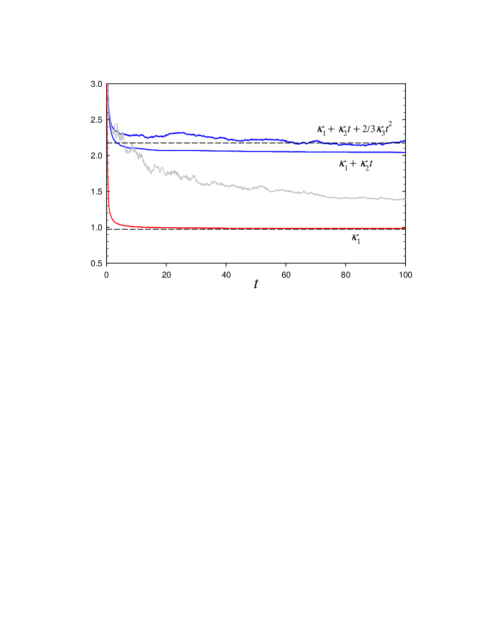
where is large enough to guarantee the convergence of the average to the desired precision. In order to obtain the asymptotic value of the generalized exponent (6), in principle, one must calculate the squared-norm averaged over several realizations at a given large time. However, we must keep in mind that such an average is dominated by the extreme positive values of the local exponent . Hence, direct averaging over may yield spurious results whenever the variance of fails to vanish with time fast enough. To avoid this problem, instead of the straightforward averaging, we preferred to estimate the local generalized exponent from the cumulants of the distribution of :
| (22) |
where are the th-order cumulants of the distribution of local exponents . Fig. 3 illustrates, for the white-noise random frequency oscillator, the as a function of time (first-order truncation of (22)), as well as the expansion (22) truncated at the second and third orders. For comparison, also plotted is the crude estimate (6). Clearly, the expansion (22) has to be considered in order to properly estimate . In Figs. 1 and 2, was numerically computed from the third-order truncation, because the next (noisier) terms do not contribute significantly.
V Correlated noise
For white noise fluctuations, either in the frequency or in the damping, we have verified in Sec. 3 (see Figs. 1 and 2), that our theory for is in agreement with numerical results, provided the later are obtained by means of the procedure described in the preceding section. The analysis in Sec. 3 also allows to quantify the discrepancy between and , which typically increases with increasing amplitude of the fluctuations.
Now we shall analyze the effect of introducing noise correlations. We consider again the case of a random frequency, as in Eq. (14), but now the noise is a zero-mean Ornstein-Ulhenbeck process, i.e., with correlation function
| (23) |
For simplicity we set and . By inserting Eq. (16) into Eq. (12), the second-cumulant matrix becomes
| (24) |
Notice that in the limit the white-noise case is recovered.
In the presence of correlations the second-order truncation of the cumulant expansion (12) is not exact. In order to improve the theory one must calculate higher cumulants. For the present case the third cumulant is null. Explicit expressions for the fourth cumulant were given by Fox [16] and by Breuer et al [32]. So, the fourth cumulant can be calculated without great effort (with the aid of algebraic manipulation programs). The fourth order approximation to reads
| (25) |
The comparison between the theoretical results for (with the second (blue) and fourth (dark blue) order corrections) and numerical outcomes is shown in Fig. 4. Notice that in numerical estimates the fourth-order correction is very small in comparison with the third-order one, suggesting that the cumulant expansion is rapidly converging.

V.1 Kubo number
The perturbation parameter controlling the convergence of the cumulant expansion is the so-called Kubo number . General considerations led van Kampen [14] to conclude that the Kubo number is the product of the amplitude of the fluctuations and the correlation time, that is . However, in the present case it is clear that such a combination is not adimensional. The correct Kubo number is instead
| (26) |
This can be checked explicitly from the second and fourth cumulants above. Consider, for instance, the element , which dominates the Lyapunov exponent for small correlation times:
| (27) |
In the white-noise limit, i.e., with fixed, the Kubo number tends to zero –as it should be.
VI Final remarks
We have taken the first step towards the application of the cumulant expansion to calculate the largest Lyapunov exponent of a dilute gas.
The case of white-noise fluctuations (either in the frequency or in the damping) was considered first. This study was very useful to understand the difficulties behind the numerical calculation of the generalized exponent . It was verified that can be obtained with a satisfactory precision by using the cumulant expansion for the distribution of the finite-time Lyapunov exponent.
We also analyzed briefly the case of correlated noise. For the Ornstein-Uhlenbeck noise we were able to obtain the fourth cumulant contribution to the analytical , which showed an improvement with respect to the second order truncation, when compared with numerical outcomes. Moreover, we showed that the correct perturbative parameter for the present problem is the product , and not , as a literal reading of van Kampen’s discussion [14] would suggest.
It is expected that the present results will be helpful for the correct application of the cumulant approach in higher dimensionality systems, as well as for the numerical checking of its validity.
Acknowledgements:
We acknowledge Brazilian agencies Faperj and CNPq for partial
financial support.
References
- [1] Krylov NS 1979 Works on the Foundations of Statistical Physics (Princeton University Press, Princeton)
- [2] Ma S-K 1985 Statistical Mechanics (World Scientific, Singapore)
- [3] Sinai YaG 1970 Russ. Math. Surv. 25 137
- [4] van Beijeren H, Dorfman JR 1995 Phys. Rev. Lett. 74 4412
- [5] van Beijeren H, Latz A, Dorfman JR 1998 Phys. Rev. E 57 4077
- [6] van Zon R, van Beijeren H, Dellago Ch 1998 Phys. Rev. Lett. 80 2035
- [7] Kruis HV, Panja D, van Beijeren H 2006 J. Stat. Phys. 124 823
- [8] Dorfman JR 1999 An Introduction to Chaos in Nonequilibrium Statistical Mechanics (Cambridge University Press, Cambridge, UK)
- [9] Dellago Ch, Posch HA, Hoover WG 1996 Phys. Rev. E 53 1485
- [10] Dellago Ch, Posch HA 1997 Physica A 240 68
- [11] Kimball JC 2001 Phys. Rev. E 63 066216
- [12] Elyutin PV 2004 Phys. Lett. A 331 153
- [13] Benettin G, Galgani L, Strelcyn J-M 1976 Phys. Rev. A 14 2338
- [14] van Kampen NG 1981 Stochastic Processes in Physics and Chemistry (North-Holland, Amsterdam)
- [15] Kubo R 1962 J. Phys. Soc. Japan 17 1100
- [16] Fox RF 1974 J. Math. Phys 15 1479
- [17] Benzi R, Paladin G, Parisi G, Vulpiani A 1985 J. Phys. A 18 2157
- [18] Castiglione P, Falcioni M, Lesne A, Vulpiani A 2008 Chaos and Coarse Graining in Statistical Mechanics (Cambridge University Press, New York, 2008)
- [19] Barnett DM, Tajima T, Nishihara K, Ueshima Y, Furukawa H 1996 Phys. Rev. Lett. 76 1812
- [20] Barnett DM, Tajima T, Nishihara K, Ueshima Y, Furukawa H 1997 Phys. Rev. E 55 3439
- [21] Barnett DM, Tajima T 1996 Phys. Rev. E 54 6084
- [22] Casetti L, Livi R, Pettini M 1995 Phys. Rev. Lett. 74 375
- [23] Casetti L, Clementi C, Pettini M, 1996 Phys. Rev. E 54 5969
- [24] Casetti L, Pettini M, Cohen EGD. 2000 Phys. Rep. 337 238
- [25] Vallejos RO, Anteneodo C 2002 Phys. Rev. E 66 021110
- [26] Anteneodo C, Maia RNP, Vallejos RO, 2003 Phys. Rev. E 68 036120
- [27] Vallejos RO, Anteneodo C 2004 Physica A 340 178
- [28] Torcini A, Dellago Ch, Posch HA 1999 Phys. Rev. Lett. 83 2676; Barnett DM, Tajima T, Ueshima Y 1999 ibid. 83 2677
- [29] Anteneodo C, Cirto L, Vallejos RO (unpublished)
- [30] Mallick K, Peyneau PE 2006 Physica D 221 72
- [31] Leprovost N, Aumaître S, Mallick K 2006 Eur. Phys. J. B 49 453
- [32] Breuer H-P, Ma A, Petruccione F 2002 preprint arXiv:quant-ph/0209153v1
- [33] Risken H 1984 The Fokker-Planck Equation: Methods of Solution and Applications (Springer-Verlag, Berlin)
- [34] Gardiner C W 1985 Handbook of stochastic methods for Physics, Chemistry and Natural Sciences (Springer-Verlag, Berlin)