Linear response formula for finite frequency thermal conductance of open systems

In many low dimensional systems, heat transport unexpectedly violates Fourier’s law of heat conduction [1, 2, 3]. This can be because of integrability or proximity to integrability, which is more common in low dimensions, as recognized starting from the Fermi-Pasta-Ulam (FPU) model [4]. Alternatively, even ergodic low-dimensional systems can show anomalous heat conduction, with the conductivity diverging with system size, if they conserve momentum. Apart from the theoretical interest, understanding heat transport in such systems is of relevance to heat conduction in carbon nanotubes [5].

Most of the recent activity [2, 3] in this field has dealt with the zero-frequency conductivity. But time dependent temperature sources have been discussed in experimental situations in the context of measuring the frequency dependent thermal conductivity [6, 7] and specific heat [8] of glassy systems. Theoretically, there have been a few studies on the frequency dependent thermal current response using a microscopic approach based on Luttinger’s derivation of the Green-Kubo formula and a hypothesis about the equality of certain transport coefficients [9], and from a phenomenological approach [10]. A recent paper studied thermal ratchet effects in an inhomogeneous anharmonic chain coupled to baths with time-dependent temperatures [11, 12].

In this paper, we adopt a different approach: we find the linear heat conductance of a system placed in contact with two heat reservoirs with time-dependent temperatures. Physically the notion of bath temperatures oscillating in time make sense if we assume that the frequency of oscillation is much smaller compared to time scales for local thermal equilibration in the reservoirs. An exact expression (in the linear response regime) for the heat current due to a small oscillating temperature difference between the reservoirs is obtained.

Our earlier result [13] obtained the zero frequency conductance of a finite system rather than the conductivity in the infinite system limit. Thus the thermodynamic limit was not taken first (in fact, not at all), in contrast to the standard Green-Kubo formula [14], which cannot be applied when the infinite system conductivity diverges. Our expression for the zero frequency conductance involved the heat current auto-correlation function for an open system. The extension to finite frequencies in this paper follows the same approach, with the response now depending on the position inside the system where the current is measured.

We also show results of numerical simulations for the frequency dependent response function by measuring the appropriate correlation function. For one-dimensional momentum conserving anharmonic crystals, we find a resonant response at a frequency $\omega\sim 1/N$ for a chain of $N$ particles due to sound waves propagating from one end of the system to the other. As $N$ increases, the resonance gets broader and its height decreases slightly. However, its height relative to the zero-frequency response increases, and for large $N$ this resonance is stronger than the zero frequency response.

We find that the low frequency peak disappears for systems where momentum is not conserved. Fourier’s law is known to be valid for such systems, so that the heat current should satisfy the diffusion equation. If one compares the numerical results for the frequency-dependent heat current with the prediction from the diffusion equation at the single bond level, there seem to be substantial discrepancies.

Numerical simulations for the frequency dependent response function of a one-dimensional harmonic crystal, and an exact analytical expression for the full response (for finite $\Delta T$) of the same, are also presented. As far as we are aware of this is the first example of a case where an analytical expression for the response function has been obtained. For a harmonic system the full response is also linear and hence we expect the linear response result to agree with the exact response function. Indeed we find excellent agreement between the numerical simulations of the expression of the linear response and the numerically evaluated exact response expression.

All three systems mentioned above also show a high-frequency peak in the response function, whose location is independent of $N.$ One can loosely ascribe this to the fact that the dynamics in the interior of the system are underdamped (actually, undamped), so that particles approaching each other recoil, and the heat current auto-correlation function shows rapid oscillations in the temporal domain. Such high-frequency oscillations are not seen in hard particle models, such as the Random Collision Model [15]. This is discussed further when we derive the analytical expression for the harmonic oscillator. However, a quantitative understanding of the high-frequency peak is lacking.

We follow the derivation of Ref. [13] to obtain the finite frequency heat conductance of an oscillator chain with Langevin baths at the ends; more detail is provided in Ref. [13]. Consider the motion of $N$ particles on a one dimensional lattice, described by the following Hamiltonian:

$$H={1\over 2}\sum_{l=1}^{N}m_{l}v_{l}^{2}+\sum_{l=1}^{N}U(x_{l}-x_{l+1})+\sum_{l=1}^{N}V(x_{l})$$

(1)

where ${\bf x}=\{x_{l}\}$ and ${\bf v}=\{v_{l}\}$ with $l=1,2,\ldots N$ are the displacements of the particles about their equilibrium positions and their velocities, and $\{m_{l}\}$ are their masses. We assume fixed boundary conditions, $x_{0}=x_{N+1}=0.$ The particles 1 and $N$ are connected to white noise Langevin heat baths at temperatures $T_{L}$ and $T_{R}.$ Thus the equations of motion are

	$\displaystyle m_{l}\dot{v}_{l}$	$\displaystyle=$	$\displaystyle-\frac{\partial}{\partial x_{l}}[U(x_{l-1}-x_{l})+U(x_{l}-x_{l+1})+V(x_{l})]$		(2)
		$\displaystyle+$	$\displaystyle\delta_{l,1}[\eta_{L}(t)-\gamma_{L}v_{1}]+\delta_{l,N}[\eta_{R}(t)-\gamma_{R}v_{N}]$

for $l=1,2,\ldots N.$ Here $\eta_{L,R}(t)$ are uncorrelated zero mean Gaussian noise terms satisfying the fluctuation dissipation relations

$$\langle\eta_{L,R}(t)\eta_{L,R}(t^{\prime})\rangle_{\eta}=2\gamma_{L,R}k_{B}T_{L,R}\delta(t-t^{\prime})~,$$

(3)

where $\langle...\rangle_{\eta}$ denotes an average over the noise.

The derivation of the linear response theory starts with the Fokker-Planck equation for the full phase space distribution function $P({\bf x};{\bf v};t)$. If $T_{L}=T_{R}=T,$ the steady state solution to the equation is the equilibrium Boltzmann distribution. We now assume that the temperatures at the two ends are oscillating in time with $T_{L,R}=T\pm\Delta T(t)/2$. We will obtain a perturbative solution about the equilibrium solution. The steps are very similar to the standard derivation of the fluctuation dissipation theorem. The Fokker Planck equation corresponding to Eq. (2) is

$$\frac{\partial P}{\partial t}=-\sum_{l}\frac{\partial}{\partial x_{l}}(v_{l}P)-\sum_{l}\frac{\partial}{\partial v_{l}}(f_{l}P/m_{l})+O_{1}P+O_{N}P$$

(4)

where $f_{l}=-\partial H/\partial x_{l}$ is the force acting on the $l$’th particle. The operators $O_{1,N}$ come from the Langevin damping and noise on the terminal particles:

	$\displaystyle O_{1}P$	$\displaystyle=$	$\displaystyle\frac{\gamma_{L}}{m_{1}}\frac{\partial}{\partial v_{1}}(v_{1}P)+\frac{\gamma_{L}k_{B}T_{L}}{m_{1}^{2}}\frac{\partial^{2}}{\partial v_{1}^{2}}P$
	$\displaystyle O_{N}P$	$\displaystyle=$	$\displaystyle\frac{\gamma_{R}}{m_{N}}\frac{\partial}{\partial v_{N}}(v_{N}P)+\frac{\gamma_{R}k_{B}T_{R}}{m_{N}^{2}}\frac{\partial^{2}}{\partial v_{N}^{2}}P.$		(5)

With $T_{L,R}=T\pm\Delta T(t)/2,$ we can group terms according to their power of $\Delta T$ to obtain

$$\frac{\partial P}{\partial t}==\hat{L}P+\hat{L}^{\Delta T}P$$

(6)

where

$$\hat{L}^{\Delta T}=\frac{k_{B}\Delta T}{2}\bigg[\frac{\gamma_{L}}{m_{1}^{2}}\frac{\partial^{2}}{\partial v_{1}^{2}}-\frac{\gamma_{R}}{m_{N}^{2}}\frac{\partial^{2}}{\partial v_{N}^{2}}\bigg].$$

(7)

For $\Delta T=0,$ the steady state solution of the Fokker Planck equation is the equilibrium Boltzmann distribution $P_{0}=\exp[-\beta H]/Z,$ where $Z$ is the canonical partition function and $\beta=1/(k_{B}T).$ For $\Delta T\neq 0,$ we start with the equilibrium distribution at time $t=t_{0}$ and then let the system evolve under the full Fokker Planck operator. Writing $P({\bf x},{\bf v},t)=P_{0}+p({\bf x},{\bf v},t)$ and retaining terms to $O(\Delta T),$

$$\frac{\partial p}{\partial t}=\hat{L}p+\hat{L}^{\Delta T}P_{0}.$$

(8)

Setting $t_{0}\rightarrow-\infty$ we get the formal solution to this equation

$$p({\bf x};{\bf v};t)=\int_{-\infty}^{t}e^{(t-t^{\prime})\hat{L}}~\Delta\beta(t^{\prime})~J_{fp}({\bf v})P_{0}({\bf x},{\bf v})dt^{\prime}$$

(9)

where $J_{fp}({\bf v})$ is defined by

$$\frac{\partial P}{\partial t}\bigg|_{P=P_{0}}=\hat{L}^{\Delta T}P_{0}=(\Delta\beta)J_{fp}P_{0}$$

(10)

from which

$$J_{fp}={\gamma_{R}\over{2m_{N}}}[m_{N}v_{N}^{2}-k_{B}T]-\frac{\gamma_{L}}{2m_{1}}[m_{1}v_{1}^{2}-k_{B}T].$$

(11)

The expectation value of any function $\langle\Delta A\rangle=\langle A\rangle-\langle A\rangle_{0}$ of any observable $A({\bf x};{\bf v})$ then takes the form:

$$\langle\Delta A(t)\rangle_{\Delta T}=-\frac{1}{k_{B}T^{2}}\int_{0}^{\infty}\langle A(\tau)J_{fp}(0)\rangle\Delta T(t-\tau)d\tau$$

(12)

where we have defined the equilibrium average $\langle A(t)J_{fp}(0)\rangle=\int d{\bf x}\int d{\bf v}Ae^{\hat{L}t}J_{fp}P_{0}$ and we have used the time translational invariance of the equilibrium correlation function. In particular, we are interested in the energy current between two adjacent particles . The instantaneous current from the $l$’th to the $l+1$’th site is given by: $j_{l+1,l}=\mbox{\small$1\over 2$}(v_{l}+v_{l+1})f_{l+1,l}$, where $f_{l+1,l}=-\partial U(x_{l}-x_{l+1})/\partial x_{l+1}$ is the force on the $l+1$’th particle due to the $l$’th particle. We get for the average heat current flowing between any bond on the chain by:

$$\langle j_{l+1,l}(t)\rangle_{\Delta T}=-\frac{1}{k_{B}T^{2}}\int_{0}^{\infty}\langle j_{l+1,l}(\tau)J_{fp}(0)\rangle\Delta T(t-\tau)d\tau.$$

(13)

For a oscillating temperature given by $\Delta T(t)=\Delta T(\omega)e^{i\omega t}$ this gives:

	$\displaystyle\frac{\langle j_{l+1,l}(\omega)\rangle}{\Delta T(\omega)e^{i\omega t}}=G_{l}(\omega)e^{-i\phi_{l}(\omega)}~~~~~~~~~~~~~~$
	$\displaystyle~~~~~=-\frac{1}{k_{B}T^{2}}\int_{0}^{\infty}\langle j_{l+1,l}(\tau)J_{fp}(0)\rangle e^{-i\omega\tau}d\tau~,~~$		(14)

where $G_{l}(\omega)$ is the magnitude of the response — to be computed numerically in Section III — and $\phi_{l}$ is the phase. The correlation function $\langle j_{l+1,l}(\tau)J_{fp}(0)\rangle$ on the right hand side of this equation is for a system in equilibrium at temperature $T.$

A few comments are appropriate here. First, as shown in Ref. [13], for $\omega\rightarrow 0$ it is possible to manipulate the integrand on the right and make it proportional to the aut-correlation function of the heat current integrated over the entire chain, $\sum_{l}j_{l+1,l}(\tau),$ yielding a result resembling the standard Green-Kubo formula (but without the thermodynamic limit). This manipulation is not possible for $\omega\neq 0.$ Thus the current response depends on $l,$ the position inside the chain where the response is measured, as one would expect. Moreover, the correlation function involves $J_{fp},$ which is different from the heat current.

Second, although we have assumed that $\Delta T_{L}=-\Delta T_{R}$ to resemble the zero-frequency calculations of Ref. [13] where such an assumption is appropriate, at $\omega\neq 0$ there is no reason why one cannot treat $\Delta T_{L}$ and $\Delta T_{R}$ as independent variables. It is straightforward to extend the derivation above and obtain the response to $\Delta T_{R}$ and $\Delta T_{L},$ with $J_{fp}$ in Eq. (14) replaced by the first and second part of Eq. (11) respectively. For large $N,$ one expects that the response to a oscillatory temperature perturbation at one end of the chain should only depend on the distance from that end and be the same as for a semi-infinite chain.

Finally, expressions similar to Eq. (13) can be obtained for any quantity that depends on the phase space variables of the system, not just $j_{l+1,l}(\tau).$ It does not apply to the heat current flowing into the system from the reservoirs, since they involve the Langevin noise $\eta_{L,R},$ and these have to be obtained indirectly. Thus Eq. (13) is valid for $l=1,$ and one also has

$$\langle d\epsilon_{1}(t)/dt\rangle_{\Delta T}=-\frac{1}{k_{B}T^{2}}\frac{d}{dt}\int_{0}^{\infty}\langle\epsilon_{1}(\tau)J_{fp}(0)\rangle\Delta T(t-\tau)d\tau.$$

(15)

Replacing the $d/dt$ with a $-d/d\tau$ acting on $\Delta T$ and integrating by parts, adding this to Eq. (13), and using the fact that $j_{21}(t)+d\epsilon_{1}(t)/dt=j_{1,L}(t)$ (where $j_{1,L}$ is the heat current flowing in from the left reservoir), we have

	$\displaystyle\langle j_{1,L}(t)\rangle_{\Delta T}$	$\displaystyle=$	$\displaystyle-\frac{1}{k_{B}T^{2}}\int_{0}^{\infty}\langle j_{1,L}(\tau)J_{fp}(0)\rangle\Delta T(t-\tau)d\tau$		(16)
		$\displaystyle-$	$\displaystyle\frac{1}{k_{B}T^{2}}\Delta T(t)\langle\epsilon_{1}(0)J_{fp}(0)\rangle.$

Fourier transforming, for $\Delta T(t)=\Delta T(\omega)e^{i\omega t},$ the heat current flowing from the left reservoir is

$$\Bigg\langle\frac{j_{1,L}(\omega)}{\Delta T(\omega)}\Bigg\rangle=-\frac{1}{k_{B}T^{2}}\int_{0}^{\infty}\langle j_{1,L}(\tau)J_{fp}(0)\rangle e^{-i\omega\tau}d\tau+\frac{\gamma_{L}}{m_{1}}k_{B}.$$

(17)

This response function has a non-zero $\omega\rightarrow\infty$ limit from the second term on the right hand side. This is reasonable: if $\Delta T$ oscillates at a very high frequency, the effect on $({\bf x},{\bf v})$ should be negligible, but the current flowing from the left reservoir should oscillate because $\langle\eta_{L}(t)v_{1}(t)\rangle_{\eta}=\gamma_{L}k_{B}T_{L}(t)/m_{1}$ is proportional to the instantaneous temperature of the reservoir. The instantaneous response of Eq. (17) is a peculiarity of white noise stochastic baths, and is not seen for Nose-Hoover baths — where even the heat current at the boundary is in terms of the extended phase space variables — or a fluid system with Maxwell boundary conditions where continuity requires that the heat current at the boundary and just inside the system should be the same. Therefore, hereafter we work with $j_{21}$ and $j_{N,N-1}$ when we want the current at the boundaries.

Although the derivation given above is for a one-dimensional chain, it is straightforward to see that it is valid for any system that is connected to only two reservoirs, regardless of its dimensionality.

Numerical simulations to obtain the correlation function on the right hand side of Eq. (14) were performed on three different systems, which differ in the potential of each particle. From these correlation functions we obtained $G_{l}(\omega)$ using Eq. (14). The velocity-Verlet algorithm was used, with a time step $\delta t=0.005.$ We verified that doubling $\delta t$ does not change our results. For the largest systems, the initial equilibration time was $t_{eq}=64\times 10^{6},$ after which the dynamical equations were evolved for a time $t=5\times 10^{8}.$ All the particle masses were set to $1$, $\gamma_{L}=\gamma_{R}=1,$ and the reservoirs were at temperature $T=2.0$. Figure 1 shows $G_{1}(\omega)$ as a function of $\omega,$ as defined by Eq. (14), for FPU chains of different lengths. The potential used was $U(x)=x^{2}/2+x^{4}/4$ with $V(x)=0.$ An $N$-independent high frequency peak and a low frequency peak at $\omega\sim 1/N$ are seen. Higher harmonics of the low frequency peak can be barely discerned. As the system size is increased, the low frequency peak broadens and decreases slightly in height, but the zero frequency response drops much faster. Thus by $N=128,$ the $\omega\sim 1/N$ resonance is clearly stronger than the zero frequency response. Note that Eq. (14) gives the conductance, not the conductivity; the $\omega=0$ conductance decreases as $\sim 1/N^{1-\alpha}$. It is expected that $\alpha=1/3$ [3] for large $N$ but this would require much larger system sizes to verify. The inset to Figure 1 shows $C_{1}(t)=\langle j_{21}(t)J_{fp}(0)\rangle,$ i.e. the same information in the time domain. $N$-independent short time oscillations that decay to (approximately) zero are seen. An ‘echo’ of the oscillation is seen at a time $\tau_{N}$ that is approximately $N/v,$ where $v$ is possibly related to the velocity of effective phonons [16].

At high frequencies, $G_{1}(\omega)$ is approximately independent of $N$ as one would expect, with a high frequency peak. As $\omega\rightarrow\infty,$ $G_{1}(\omega)\sim 1/\omega^{2}.$

Figure 2 shows $G_{2}(\omega),$ the magnitude of the response function at a distance $l=2$ from the left boundary. The low frequency peak (and its harmonics) are still present, but much more irregular in shape. However, from a device perspective, it is the currents flowing into the boundaries that are important.

The high frequency behavior is independent of $N,$ and as seen in the inset, the peak in $G_{l}(\omega)$ shifts to smaller $\omega$ as $l$ is increased. It is not clear if $G_{2}(\omega\sim\infty)\sim 1/\omega^{6}$ as is seen for the harmonic chain (discussed later in this paper).

Figure 3 shows $G_{1}(\omega)$ for chains of different lengths with an onsite potential $V(x)=x^{4}/4.$ The interparticle potential is harmonic, $U(x)=x^{2}/2.$ The dynamics are not momentum conserving, and the zero frequency conductance should be inversely proportional to $N.$ This is not seen in the data for two reasons: direct measurement of the zero frequency conductance by applying a small temperature difference between the reservoirs shows that one needs $N\gtrsim 256$ to see the $\sim 1/N$ dependence, and the curves for the two larger systems (more noticeably $N=128$) have not reached their $\omega\rightarrow 0$ limit in the figure. The low frequency resonance is gone, replaced by a broad $N$-independent plateau. This is presumably because at finite temperature, the effective phonons are optical instead of acoustic. The $N$-independent high frequency peak is also present. The response in the interior of the chain, shown in Figure 4 is similar, except that the low frequency plateau extends down to $\omega=0$ (or to very small $\omega$). As for the FPU chains, we fit $G_{1}(\omega\sim\infty$ to $\sim 1/\omega^{2}$ and — less successfully — $G_{2}(\omega\rightarrow\infty)$ to $\sim 1/\omega^{6}.$

From the inset to Figure 4, there is no significant $l$-dependence to the location of the high frequency peak in $G_{l}(\omega)$, unlike what we saw for FPU chains.

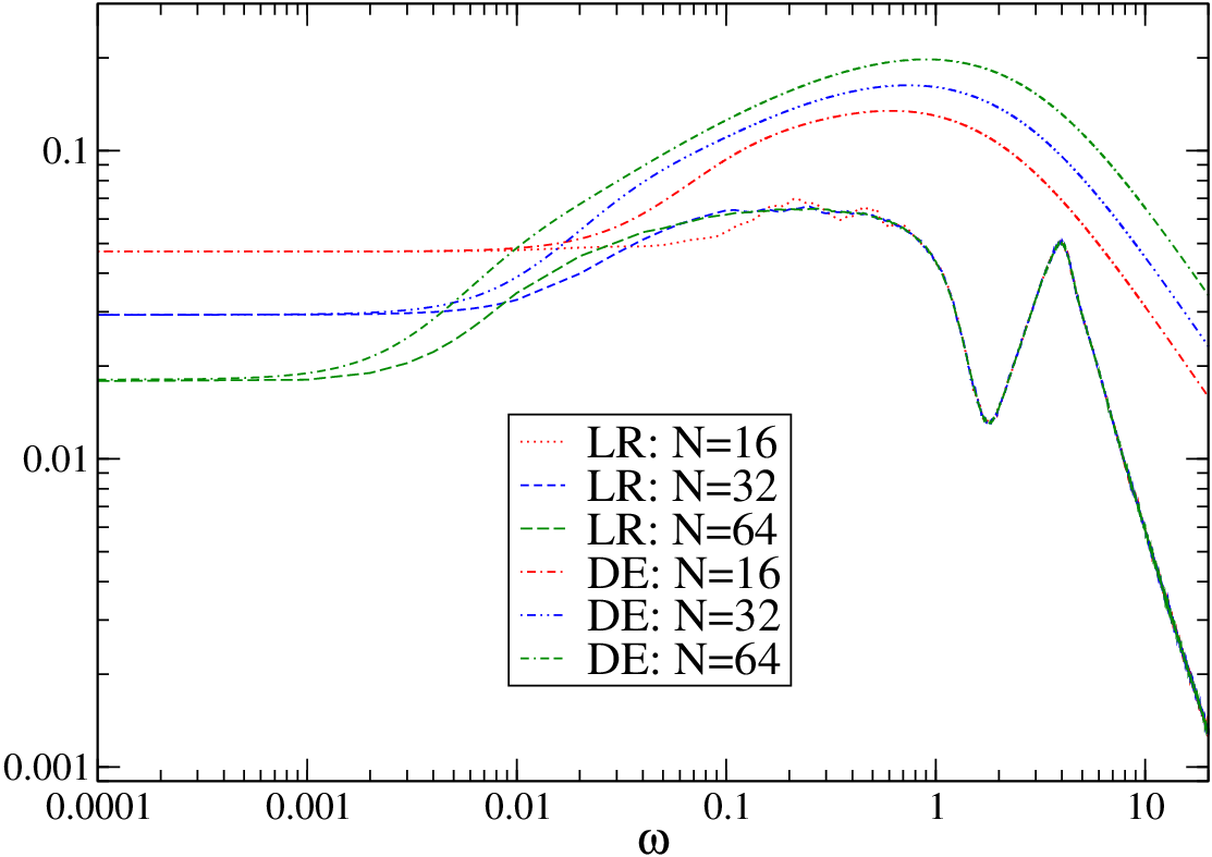
Beyond the $\sim 1/N$ dependence of the zero frequency conductance, one expects that heat transport in systems that are not momentum conserving should be diffusive, and the temperature field will satisfy $\partial T_{l}/\partial t=D(T_{l+1}-2T_{l}+T_{l-1})$ where $D=\kappa/C$ is the diffusion constant. With an $\sim e^{i\omega t}$ time dependence, the resultant difference equation can be solved with $T_{L}(\omega)$ and $T_{R}(\omega)$ specified, and thence the heat current $j_{l+1,l}=\kappa(T_{l}-T_{l+1})$ can be calculated. Some features of the solution are $G^{\rm diff}_{l}(\omega=0)\propto 1/N,$ $G^{\rm diff}_{l}(\omega)$ is independent of $N$ for $N\rightarrow\infty,$ $G^{\rm diff}_{l}(\omega\rightarrow 0)\sim\omega^{1/2}\exp[-(\omega/2D)^{1/2}l]$ and $G^{\rm diff}_{l}(\omega\rightarrow\infty)\sim 1/\omega^{l}.$ In Figure 5 we plot the responses $G^{\rm diff}_{1}$ together with the linear response results $G_{1}$ for the $\phi^{4}$ model. For each system size we fix the diffusion constant $D$ so that the $\omega=0$ results for the two responses match. One expects that the low-frequency agreement between the two sets should become better with increasing system size. However this is not clear from our data. At high frequencies, the expectation $G^{diff}_{1}(\omega)\sim 1/\omega$ is definitely not borne out. Since the diffusion equation is not expected to be valid at microscopic time or length scales, and the fact that $\sim 1/N$ scaling of the zero frequency heat conductance is only seen for $N\gtrsim 256$ suggests that ‘microscopic’ length scales are quite large here, the lack of agreement at the single bond level and high frequencies is perhaps not surprising. A clear understanding of this requires further work.

Finally, we show the results for a harmonic chain, with $V(x)=0$ and $U(x)=x^{2}/2.$ In this case we show in the next section [sec. (IV)] that the response $G_{l}(\omega)$ can be obtained exactly and expressed in terms of a single integral over frequencies. Here we give numerical results for $G_{l}(\omega)$ obtained using this exact formula [Eq. (21)] and also compare it with the linear response result [Eq. (14)]. We show $G_{1}(\omega)$ in Figure 6, with results from numerical simulations of the linear response formula also shown for $N=64$. We see excellent agreement between the analytical and linear response result. One can see that $G_{1}(\omega=0)$ is almost $N$-independent as expected, and the low frequency resonance and its harmonics are more pronounced than for the FPU chain, which is not surprising since there is no dispersion or damping in the interior of the chain. The high frequency peak seems to be present but is difficult to cleanly separate from the low frequency structure. As was the case for the FPU and $\phi^{4}$ chains, $G_{1}(\omega\rightarrow\infty)$ is $N$-independent and $\sim 1/\omega^{2}.$ In Section IV, the asymptotic form $G_{l}(\omega\rightarrow\infty)\sim 1/\omega^{4l-2}$ is obtained. Figure 7 shows $G_{2}(\omega)$ for various system sizes, with all features as expected.

Although the integrability of the harmonic oscillator chain makes its behavior non-generic, and its applicability to physical systems limited, the advantage of this model is that its response can be completely obtained analytically (with some integrals evaluated numerically) and compared to the simulation results. We now proceed with the analysis.

In this case both $V(x)$ and $U(x)$ are quadratic and the Hamiltonian can be written in the form $H=\dot{X}M\dot{X}/2+X\Phi X/2$ where $M$ and $\Phi$ are respectively the mass matrix and the force-constant matrix for the system. We will obtain the solution of the equations of motion in the time-dependent steady state by using Fourier transforms in the time domain. The approach is similar to that used in the derivation of the Landauer-type formula for steady state heat current in harmonic systems, where the current is expressed in terms of phonon Green’s functions [17]. Let us introduce the transforms: $\tilde{x}_{l}(\Omega)=(1/2\pi)\int_{-\infty}^{\infty}dtx_{l}(t)e^{i\Omega t}$ and $\tilde{\eta}_{L,R}(\Omega)=(1/2\pi)\int_{-\infty}^{\infty}dt\eta_{L,R}(t)e^{i\Omega t}$. Then the Fourier transform solution of Eqns. (2) gives:

$\displaystyle\tilde{x}_{l}(\Omega)=\mathcal{G}_{l1}^{+}(\Omega)\tilde{\eta}_{L}(\Omega)+\mathcal{G}_{lN}^{+}(\Omega)\tilde{\eta}_{R}(\Omega)~,$

(18)

where $\mathcal{G}^{+}(\Omega)=[-M\Omega^{2}+\Phi-\Sigma^{+}(\Omega)]^{-1}$ is the phonon Green’s function [17] and $\Sigma^{+}$, the self-energy correction due to baths, is a $N\times N$ matrix whose only non-zero elements are $\Sigma^{+}_{11}=i\Omega\gamma_{L},~\Sigma^{+}_{NN}=i\Omega\gamma_{R}$. The noise correlations corresponding to the oscillating temperatures $T_{L}=T+\Delta T/2\cos\omega t,~T_{R}=T-\Delta T/2\cos\omega t$ are given by:

			$\displaystyle\langle\tilde{\eta}_{L}(\Omega_{1})\tilde{\eta}_{L}(\Omega_{2})\rangle=\frac{\gamma_{L}k_{B}}{\pi}\{~T~\delta(\Omega_{1}+\Omega_{2})$		(19)
		$\displaystyle+$	$\displaystyle(\Delta T/4)[~\delta(\Omega_{1}+\Omega_{2}+\omega)+\delta(\Omega_{1}+\Omega_{2}-\omega)~]~\}~,$
			$\displaystyle\langle\tilde{\eta}_{R}(\Omega_{1})\tilde{\eta}_{R}(\Omega_{2})\rangle=\frac{\gamma_{R}k_{B}}{\pi}\{~T\delta(\Omega_{1}+\Omega_{2})$
		$\displaystyle-$	$\displaystyle(\Delta T/4)[~\delta(\Omega_{1}+\Omega_{2}+\omega)+\delta(\Omega_{1}+\Omega_{2}-\omega)~]~\}~,~~$

and $\tilde{\eta}_{L},\tilde{\eta}_{R}$ are uncorrelated. The heat current on any bond is given by the noise average $\langle j_{l+1,l}\rangle=\langle(1/2)\langle k(x_{l}-x_{l+1})(v_{l}+v_{l+1})\rangle,$ where $k$ is the force constant of the bonds, and thus involves evaluating

			$\displaystyle\langle x_{l}(t)v_{m}(t)\rangle=\int_{-\infty}^{\infty}d\Omega_{1}\int_{-\infty}^{\infty}d\Omega_{2}~(-i\Omega_{2})~e^{-i(\Omega_{1}+\Omega_{2})t}$		(20)
			$\displaystyle\times\big[~\mathcal{G}_{l1}^{+}(\Omega_{1})\mathcal{G}_{m1}^{+}(\Omega_{2})~\langle\tilde{\eta}_{L}(\Omega_{1})\tilde{\eta}_{L}(\Omega_{2})\rangle$
		$\displaystyle+$	$\displaystyle\mathcal{G}_{lN}^{+}(\Omega_{1})\mathcal{G}_{mN}^{+}(\Omega_{2})~\langle\tilde{\eta}_{R}(\Omega_{1})\tilde{\eta}_{R}(\Omega_{2})\rangle~\big]$

and this is readily evaluated using the noise properties in Eq. (19). After some simplifications we finally obtain:

	$\displaystyle G_{l}(\omega)$	$\displaystyle=$	$\displaystyle\big|~\frac{1}{4\pi}\int_{-\infty}^{\infty}d\Omega~\Omega$		(21)
		$\displaystyle\times$	$\displaystyle\big[\gamma_{L}\big\{\mathcal{G}^{+}_{l,1}(\Omega-\omega)-\mathcal{G}^{+}_{l+1,1}(\Omega-\omega)\big\}$
			$\displaystyle~~~~~~\times\big\{\mathcal{G}^{+}_{l,1}(-\Omega)+\mathcal{G}^{+}_{l+1,1}(-\Omega)\big\}$
		$\displaystyle-$	$\displaystyle\gamma_{R}\big\{\mathcal{G}^{+}_{l,N}(\Omega-\omega)-\mathcal{G}^{+}_{l+1,N}(\Omega-\omega)\big\}$
			$\displaystyle~~~~~~\times\big\{\mathcal{G}^{+}_{l,N}(-\Omega)+\mathcal{G}^{+}_{l+1,N}(-\Omega)\big\}\big]~\big|~.$

For nearest neighbor interactions, the force matrix $\Phi$ is a tri-diagonal matrix. Using the properties of inverse of a tri-diagonal matrix we can explicitly evaluate the Green’s function elements that are required. For simplicity consider the case $k=1$ and $\gamma_{L}=\gamma_{R}=\gamma$. Let us define $\Delta_{l,m}$ as the determinant of the sub-matrix of $[-M\Omega^{2}+\Phi-\Sigma^{+}]$ that starts from the $l^{\rm th}$ row and column and ends in the $m^{\rm th}$ row and column. We also define $D_{l,m}$ as the determinant of the sub-matrix of $[-M\Omega^{2}+\Phi]$ starting from the $l^{\rm th}$ row and column and ending in the $m^{\rm th}$ row and column. In terms of these one has:

$\displaystyle\mathcal{G}^{+}_{l,1}(\Omega)$

$\displaystyle=$

$\displaystyle\frac{\Delta_{l+1,N}}{\Delta_{1,N}},~~\mathcal{G}^{+}_{l,N}(\Omega)=\frac{\Delta_{1,l-1}}{\Delta_{1,N}}$

with

	$\displaystyle\Delta_{1,l-1}$	$\displaystyle=$	$\displaystyle D_{1,l-1}-i\Omega\gamma D_{2,l-1}$
	$\displaystyle\Delta_{l+1,N}$	$\displaystyle=$	$\displaystyle D_{l+1,N}-i\Omega\gamma D_{l+1,N-1}$
	$\displaystyle\Delta_{1,N}$	$\displaystyle=$	$\displaystyle D_{1,N}-i\Omega\gamma(D_{1,N-1}+D_{2,N})-\Omega^{2}\gamma^{2}D_{2,N-1}~.$

For an ordered harmonic chain with all masses equal to $1$ it is easy to show that $D_{l,m}=\sin(m-l+2)q/\sin q$ where $\Omega^{2}=2(1-\cos q)$. Using this it is easy to numerically evaluate the response function $G_{l}(\omega)$ in Eq. (21) for given values of $l,N$. We show some numerical results in Figs. (6,7) where we have also compared with results from simulations for the linear response. As expected the exact response and the linear response give almost identical results. However we have not been able to analytically show the equivalence of the exact response and the linear response expressions.

For large $\Omega$, we have $q\sim\pi+i\ln\Omega^{2}$, hence

$$\mathcal{G}^{+}_{l,1}(\Omega)\sim 1/(-\Omega^{2})^{l}.$$

(22)

This can also be seen from the equations of motion: when $\Omega>>0,$ the dynamical equations become $-m_{l}\Omega^{2}x_{l}=kx_{l-1}.$ The boundary condition is $-m_{1}\Omega^{2}x_{1}=\eta_{L}(\Omega),$ in which the right hand sign is effectively unity when calculating the Green’s function. Combining these equations, we obtain Eq. (22). But a $\sim 1/(-\Omega^{2})^{l}$ dependence at large frequencies implies that the $2l$’th derivative of $\mathcal{G}^{+}_{l,1}(t)$ has a $\delta$-function at the origin, i.e. $\mathcal{G}^{+}_{l,1}(t)\sim t^{2l-1}$ for $t\gtrsim 0$ (This can be verified directly in the time domain: $x_{l}(t)\propto t^{2l-1}$ satisfies the equations of motion for $t\gtrsim 0.$) But then in the time domain, Eq. (21) is equivalent to $G_{l}(t)\propto\mathcal{G}^{+}_{l,1}(t)\partial_{t}\mathcal{G}^{+}_{l,1}(t)$ for $t\gtrsim 0,$ where we have assumed that $l$ is in the left half of the chain. Therefore $G_{l}(t\gtrsim 0)\propto t^{4l-3}.$ Since $G_{l}(t<0)=0,$ the $4l-2$’th derivative of $G_{l}(t)$ has a $\delta$-function at $t=0,$ so that

$$G_{l}(\omega)\sim 1/\omega^{4l-2}\qquad l<N/2$$

(23)

for large $\omega.$

In this paper, we have given an exact linear response formula for the current in a wire in response to time-dependent temperatures applied at the boundaries. For a harmonic chain the full response function has been analytically computed. We have presented numerical results for the frequency dependence of the current response in oscillator chains. For a diffusive system we find that the response differs from what is expected from a solution of the Fourier’s equation with oscillating boundary temperatures. It is straightforward to generalize the derivation to fluid systems, various stochastic and deterministic baths, and arbitrary system size $L$ and spatial dimension $d.$ This is discussed in detail in Ref. [13] for the $\omega=0$ case.

As shown in Ref. [13] the zero frequency response can be expressed in terms of current auto-correlation functions, resulting in an expression similar to the standard Green-Kubo formula but without the thermodynamic limit being taken. If the integral of the auto-correlation function remains finite in the thermodynamic limit, the conductance is $\sim 1/N$ for large $N,$ and one can define an $N$-independent conductivity in the same regime. The resultant expression matches the standard Green-Kubo formula, but with the thermodynamic limit taken after the range of the integral is taken to infinity. While it is plausible to assume that the order of limits commutes and

$$\lim_{L\rightarrow\infty}\frac{1}{L}\lim_{t_{0}\rightarrow\infty}\int_{0}^{t_{0}}C_{JJ}(t)dt=\lim_{t_{0}\rightarrow\infty}\lim_{L\rightarrow\infty}\frac{1}{L}\int_{0}^{t_{0}}C_{JJ}(t)dt,$$

(24)

this is by no means trivial: if different boundary conditions had been employed, with hard wall boundaries instead of heat baths, the left hand side of this equation is zero but the right hand side is not. If the left hand side (with heat bath boundary conditions) diverges in the thermodynamic limit, as for integrable systems or low dimensional momentum conserving systems, the conductivity also diverges, and one can only talk about the conductance or an $L$-dependent conductivity.

At non-zero frequencies, the integral converges even when it does not at $\omega=0,$ and changing the order of limits is more benign. Unfortunately, as we have seen in this paper, the expression obtained for the finite frequency conductance involves the correlation function $\langle j_{l+1,l}(\tau)J_{fp}(0)\rangle,$ which we are unable to convert into an auto-correlation function when $\omega\neq 0.$ The connection to proposed expressions for the finite frequency conductivity [9, 10] is not clear.

References

- [1] F. Bonetto, J.L. Lebowitz, and L. Rey-Bellet, “Fourier’s Law: A Challenge to Theorists,” Mathematical Physics 2000 (Imp. Coll. Press, London, 2000).
- [2] S. Lepri, R. Livi and A. Politi, Phys. Rep. 377, 1 (2003).
- [3] A. Dhar, Adv. Phys. 57, 457 (2008).
- [4] E. Fermi, J. Pasta, and S. Ulam, Studies of nonlinear problems (Los Alamos Document LA-1940, 1955).
- [5] C.W. Chang, D. Okawa, H. Garcia, A. Majumdar and A. Zettl, Phys. Rev. Lett. 101, 075903 (2008); D Li, Y Wu, P Kim, L Shi, P Yang, A Majumdar, Appl. Phys. Lett. 83, 2934 (2003).
- [6] P. K. Dixon and S. R. Nagel, Phys. Rev. Lett. 61, 341 (1988).
- [7] J. S. Olafsen and R. P. Behringer, J. of Low Temp. Phys., 117, 53 (1999).
- [8] N. O. Birge, Phys. Rev. B 34, 1631 (1986).
- [9] B. S. Shastry, Phys. Rev. B 73, 085117 (2006).
- [10] S. G. Volz, Phys. Rev. Lett. 87, 074301 (2001).
- [11] N. Li, P. Hanggi and B. Li, Euro. Phys. Lett. 84, 40009 (2008).
- [12] J. Ren and B. Li, Phys. Rev. E 81, 021111 (2010).
- [13] A. Kundu, A. Dhar and O. Narayan, J. Stat. Mech. L03001 (2009).
- [14] M.S. Green, J. Chem. Phys. 22, 398 (1954); R. Kubo, M. Yokota and S. Nakajima, J. Phys. Soc. Japan 12, 1203 (1957).
- [15] J.M. Deutsch and O. Narayan, Phys. Rev. E 68, 041203 (2003).
- [16] N. Li, B. Li and S. Flach, Phys. Rev. Lett. 105, 054102 (2010).
- [17] A. Dhar and D. Roy, J. Stat Phys. 125, 801 (2006).