For completeness we list definitions of the various form factors. The Dirac and Pauli form factors, $F^{N}_{1}$ and $F^{N}_{2}$, respectively, are defined by [21, 22]

where $q^{2}=(p^{\prime}-p)^{2}=t$ and $N$ stands for $p$ or $n$. The Sachs electric and magnetic form factors are related to the Dirac-Pauli basis by [23]

At $t=0$ they are [5] $G^{p}_{E}(0)=1$, $G^{n}_{E}(0)=0$, $G^{p}_{M}(0)=\mu_{p}\approx 2.793$, $G^{n}_{M}(0)=\mu_{n}\approx-1.913$. We write the isoscalar and isovector form factors as

such that at $t=0$ they are, $G_{E}^{(0)}(0)=1$, $G_{E}^{(1)}(0)=1$, $G_{M}^{(0)}(0)=\mu_{p}+\mu_{n}$ $G_{M}^{(1)}(0)=\mu_{p}-\mu_{n}$. Notice that $G^{(0)}_{E,M}=2G^{s}_{E,M}$, $G^{(1)}_{E,M}=2G^{v}_{E,M}$ for $G^{s,v}_{E,M}$ of [26].

The analytic structure in the $t$ plane illustrated in Fig. 1 implies the dispersion relation,

Knowledge of ${\rm Im}G_{E}^{p}$ over the cut translates into information about the coefficients in the $z$ expansion. We begin with a general discussion of these relations.

Let us consider a general function with the analytic structure as in Fig. 1, $G(t)=\sum_{k=0}^{\infty}a_{k}z(t)^{k}$. Equation (2) maps points just above (below) the cut in the $t$ plane onto points in the lower (upper) half unit circle in the $z$ plane. Parameterizing the unit circle by $z(t)=e^{i\theta}$ and solving (2) for $t$, we find

We can now use the orthogonality of $z^{k}$ over the unit circle to find

Since $G$ is analytic, $a_{k}=0$ for $k<0$, and therefore

The coefficients in the expansion (3) can also be used to construct a norm of the form factor in the mathematical sense. To keep the discussion general, let us introduce a function $\phi$ sharing the domain of analyticity of $G$, and write

Consider the class of norms specified by

In particular, the “uniform norm” is equal to the maximum coefficient size, $||\phi G||_{\infty}=\sup_{k}{|a_{k}|}=\lim_{p\to\infty}||\phi G||_{p}$. The case $p=2$ is of special interest since the norm is easily related to a dispersion integral,

The finiteness of $||\phi G||_{2}$ shows that the coefficients $a_{k}$ are not only bounded, but must decrease in size for sufficiently large $k$. The relation $||\phi G||_{\infty}\leq||\phi G||_{2}$ indicates that $||\phi G||_{2}$ may overestimate the actual size of the relevant coefficients in certain cases. We proceed to consider a vector dominance model to illustrate this feature and then turn to a more detailed analysis of the spectral functions.

In many applications, the $||\cdot||_{2}$ norm is used in conjunction with “unitarity bounds” obtained by identifying the dispersive integral with a physical production rate. In the present example, dominant contributions to the integral arise from the region below the two-nucleon production threshold, and we must turn to different methods of analysis. For example, employing a vector dominance ansatz in the appropriate channel, Table 2 displays estimates for the quantity $||\phi G||_{2}/\phi(t_{0})G(t_{0})=\sqrt{\sum_{k}{a_{k}^{2}/a_{0}^{2}}}$, for different choices of the functional form of $\phi$ and the value of $t_{0}$ ⁶⁶ 6 For this purpose we estimate $G_{E}(t_{0})$ using a dipole ansatz for the form factor, $G_{E}(t)\sim 1/(1-t/0.71\,{\rm GeV}^{2})^{2}$. . The effects of the leading resonance in each channel are represented by a Breit Wigner profile [24],

with $\alpha_{1}\approx 1$, $\alpha_{2}\approx-0.12$, $m_{\omega}=783\,{\rm MeV}$, $\Gamma_{\omega}=8.5\,{\rm MeV}$ for the isoscalar channel; and $\beta_{1}\approx 1$, $\beta_{2}\approx 3.7$, $m_{\rho}=775\,{\rm MeV}$, $\Gamma_{\rho}=149\,{\rm MeV}$ for the isovector channel. At $\Gamma=0$, the ansatz is normalized to the $t=0$ values in Section 3.1.

We note that in the isoscalar case, the rather large size of the estimated norm is due to the narrow width of the $\omega$ resonance; in fact, in the limit of an infinitely narrow resonance, the quantity $||G||_{2}$ diverges, as seen from (18). Closer examination indicates that the large norm is due not to the coefficients growing in size, but rather to a sequence of coefficients whose slow fall-off causes a slow convergence for the sum $\sum_{k}a_{k}^{2}$. A straightforward computation shows that the expansion coefficients for an infinitely narrow pole, $G(t)=G(0)/(1-t/m_{V}^{2})$, are for $k\geq 1$,

In particular, $|a_{k}/a_{0}|\leq 2\sqrt{(t_{\rm cut}-t_{0})/(m_{V}^{2}-t_{\rm cut})}$. This approximation to the uniform norm is also displayed in Table 2.

Equations (15) and (18) are model-independent, whereas the approximations based on the vector dominance ansatz employed in Table 2 are model dependent. This ansatz aims simply to capture the order of magnitude of the coefficients, which is sufficient in practice to constrain the form factor fits. The conclusion is that $|a_{k}|\leq 10$ is a very conservative estimate for this ansatz.

We can be more explicit in the case of the isovector form factor expansion, where the leading singularities are due to $\pi\pi$ continuum contributions that are in principle constrained by measured $\pi\pi$ production and $\pi\pi\to N\bar{N}$ annihilation rates [6, 25, 26]:

where $F_{\pi}(t)$ is the pion form factor (normalized according to $F_{\pi}(0)=1$) and $f^{1}_{+}(t)$ is a partial amplitude for $\pi\pi\to N\bar{N}$. Using that these quantities share the same phase [25], we may substitute absolute values. Strictly speaking, this relation holds up to the four-pion threshold, $t\leq 16m_{\pi}^{2}$. For the purposes of estimating coefficient bounds, we will take the extension of (21) assuming phase equality through the $\rho$ peak as a model for the total $\pi\pi$ continuum contribution.

For $|F_{\pi}(t)|$ we take an interpolation using the four $t$ values close to production threshold from [27] ($0.101$ to $0.178\,{\rm GeV}^{2}$), and 43 $t$ values from [28] ($0.185$ to $0.94\,{\rm GeV}^{2}$). Values for $f_{+}^{1}(t)$ are taken from Table 2.4.6.1 of [29]. Evaluating (15) using (21) and the experimental data up to $t=0.8\,{\rm GeV}^{2}\approx 40\,m_{\pi}^{2}$ yields for the first few coefficients, at $\phi=1$ and $t_{0}=0$: $a_{0}\approx 2.1$ $a_{1}\approx-1.4$, $a_{2}\approx-1.6$, $a_{3}\approx-0.9$, $a_{4}\approx 0.2$. Using $|\sin(k\theta)|\leq 1$ in the integral gives $|a_{k}|\lesssim 2.0$ for $k\geq 1$.

The leading singularities in the isoscalar channel could in principle be analyzed using data for the $3\pi$ continuum. Since we do not attempt to raise the isoscalar threshold in our analysis, we content ourselves with a simple vector dominance model to estimate the coefficient bounds. The first few coefficients for the isoscalar form factor using (20) for a narrow $\omega$ resonance are: $a_{0}=1$, $a_{1}\approx-1.2$, $a_{2}\approx-0.96$, $a_{3}\approx 0.4$, $a_{4}\approx 1.3$. We will compare the above values to those extracted from electron scattering data later. For the moment we note that a bound $|a_{k}|\leq 10$ is conservative.

Let us return to the choice of $\phi$. We will consider three essentially different choices. First, $\phi(t)=1$ is our default choice. We noted that for $\phi=1$ the dominant contributions to $||\phi G||_{2}$ are from narrow resonances. We could negate the large contribution of the leading resonances by using for $\phi$ the inverse of a vector meson dominance (VMD) form factor. As a second choice, consider

where $m_{V}$ is the mass of the leading resonance in the appropriate channel, i.e., $\rho(770)$ for the isovector, $\omega(780)$ for the isoscalar. Note that using $G_{E}\sim 1/t^{2}$ at large $t$, the dispersion integral remains convergent. There is no loss of model-independence here, since corrections to vector dominance are accounted for in the coefficients $a_{k}$. As discussed in Section 3.6, a third choice of $\phi$ is motivated by unitarity and an operator product expansion (OPE):

where $t_{\rm cut}$ is appropriate to the chosen isospin channel. For definiteness, we choose $Q_{\rm OPE}^{2}=1\,{\rm GeV}^{2}$ in the unitarity-inspired $\phi$. In our final fits, we focus on $\phi=1$ and $t_{0}=0$ but demonstrate that the results are essentially unchanged for different choices.

The contribution of the physical region $t\geq 4m_{N}^{2}$ to $||\phi G_{E}||_{2}$ is

The cross section for $e^{+}e^{-}\to N\bar{N}$ is [30]

and thus for the proton electric form factor we have

where $\sigma_{0}=4\pi\alpha^{2}/3t$ and $v(t)=\sqrt{1-4m_{N}^{2}/t}$ is the nucleon velocity in the center-of-mass frame. Using the data from [31] (see also [32, 33]), we can perform the integral from $t=4.0\,{\rm GeV}^{2}$ to $9.4\,{\rm GeV}^{2}$ assuming $|G_{M}^{p}/G_{E}^{p}|\lesssim 1$.⁷⁷ 7 For $|G_{M}/G_{E}|\geq 1$, the quantity in square brackets in (26) is bounded by the quantity denoted by $|G|^{2}$ in [31]. This inequality is satisfied experimentally in the $t$ range of interest. At $t_{0}=0$ and $\phi=1$, we find the result $\delta||G_{E}^{p}||^{2}_{2}\lesssim(0.03)^{2}$, to be added to the contribution from $t\leq 4m_{N}^{2}$. This result is obtained by using for $\sigma(t)$ the measured central value plus $1\sigma$ error. The remaining integral above $t=9.4\,{\rm GeV}^{2}$ can be conservatively estimated by assuming a constant form factor beyond this point, yielding an additional $\delta||G_{E}^{p}||_{2}^{2}\approx(0.008)^{2}$. The neutron form factor can be treated similarly using the data from [34] for $t=3.61$ to $5.95\,{\rm GeV}^{2}$. This leads to $\delta||G_{E}^{n}||^{2}_{2}\approx(0.05)^{2}$. The remainder at high $t$ assuming a constant form factor yields an additional $\delta||G_{E}^{n}||_{2}^{2}\approx(0.05)^{2}$. Similarly, using $|{\rm Im}G_{E}\sin k\theta|\leq|G_{E}|$ the contribution of the timelike region to (15) is small: $|\delta a_{k}|\lesssim 0.011+0.004$ for the proton, and $|\delta a_{k}|\lesssim 0.013+0.025$ for the neutron. We conclude that when estimating the bounds on coefficients, the physical timelike region can be safely neglected.

Let us mention that we can bound the contribution of the physical timelike region by a perturbative quark-level computation. Decompose the electromagnetic current correlation function as

and define

The two-nucleon contribution to the correlator satisfies

and hence with $\phi G_{E}=\sum_{k}a_{k}z^{k}$ and the choice of $\phi$ in (23),

If we choose $Q_{\rm OPE}^{2}$ large enough, the function $\chi(Q_{\rm OPE}^{2})$ is perturbatively calculable as an operator product expansion: $\chi\approx\sum_{f}e_{f}^{2}/8\pi^{2}Q_{\rm OPE}^{2}$ at leading order, where $e_{f}$ denotes the electric charge of a given quark flavor. Choosing for illustration $Q_{\rm OPE}^{2}=1\,{\rm GeV}^{2}$, $n_{f}=3$ light quark flavors, and $t_{\rm cut}=4m_{\pi}^{2}$, we find the bounds $\delta(\sum_{k}a_{k}^{2})\sim(1.0)^{2}$ for $t_{0}=0$ and $\delta(\sum_{k}a_{k}^{2}/a_{0}^{2})\sim(1.4)^{2}$ for $t_{0}=t_{0}^{\rm opt}(0.5\,{\rm GeV}^{2})$. We note that these “unitarity bounds” overestimate the contribution from the physical region $t\geq 4m_{N}^{2}$, due both to subthreshold resonance production, and to other channels, e.g., $N\bar{N}$ plus pions, above threshold. For this reason, we do not dwell on a more precise analysis of this bound, or on a separation into definite isospin channels.

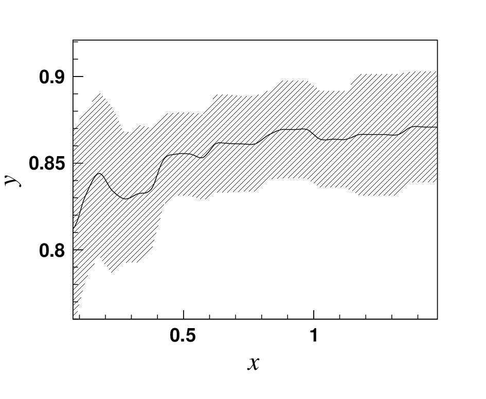
We have argued that, taking the data tabulated in [19] at face value, the final entry in Table 1 is a model-independent determination of the proton charge radius: $r_{E}^{p}=0.878^{+0.039}_{-0.062}\,{\rm fm}$. In the absence of further model-independent constraints on the form factors, obtaining a proton charge radius with smaller error requires further experimental input. Here we investigate the impact of higher-$Q^{2}$ proton scattering data.

Figure 3 shows the central value and $1\sigma$ ($\Delta\chi^{2}=1$) error band obtained by fitting the electron-proton scattering data compiled by Arrington et al. [7]. We take $\phi=1$ and $t_{0}=0$, and include as many coefficients $a_{k}$ as necessary for the fits to stabilize. As the figure illustrates, for $Q^{2}\gtrsim{\rm few}\times 0.1\,{\rm GeV}^{2}$ the impact of additional data is minimal. While an ever greater number of coefficients $a_{k}$ at higher $k$ must be included to obtain convergence, the total error on the slope at $Q^{2}=0$ is not reduced. For later use, we note that the coefficients $a_{k=1,2,3}$ extracted from the fit at $Q^{2}_{\rm max}=1\,{\rm GeV}^{2}$ are $-1.01(6)$, $-1.4^{+1.1}_{-0.7}$, $2^{+2}_{-6}$.

We can separate the isoscalar from the isovector form factor, making use of the fact that the isoscalar cut is further away from $t=0$ than the isovector cut, translating to a smaller value of $|z|_{\rm max}$ as discussed in the Introduction. A combined fit of proton and neutron data can then be performed. For the proton form factor we again use the data from [7]. For the neutron electric form factor, we use 20 data points from [35, 36, 37, 38, 39, 40, 41, 42, 43, 44, 45, 46]. We take as additional input the neutron charge radius from neutron-electron scattering length measurements [5]:

Table 3 shows the effect of different expansion schemes (choices of $\phi$ and $t_{0}$) and coefficient bounds on the form factor slope determination. For later use, the coefficients $a_{k=1,2,3}$ extracted from the fit for $Q^{2}_{\rm max}=1\,{\rm GeV}^{2}$, $\phi=1$, $t_{0}=0$ and $k_{\rm max}=8$ are $-1.99^{+0.13}_{-0.12}$, $0.3^{+1.5}_{-1.9}$, $-2^{+9}_{-6}$ for the isoscalar channel; and $-1.20^{+0.06}_{-0.05}$, $-0.6^{+1.3}_{-1.2}$, $-2^{+6}_{-7}$ for the isovector channel. The sign and approximate magnitude of the first coefficients agree with the $\pi\pi$ continuum model, and the narrow-width $\omega$ resonance model mentioned in Section 3.4.

We can effectively raise the isovector threshold by including the $\pi\pi$ continuum explicitly, as constrained by $\pi\pi$ production and $\pi\pi\to N\bar{N}$ data:

where $G_{\rm cut}(t)$ is generated by (21) for $4m_{\pi}^{2}<t<16m_{\pi}^{2}$. For $|F_{\pi}(t)|$ we take the four $t$ values close to production threshold from [27] ($0.101$ to $0.178\,{\rm GeV}^{2}$), and twelve $t$ values from [28] ($0.185$ to $0.314\,{\rm GeV}^{2}$). The product of the remaining kinematic factor and $f^{1}_{+}$ from [29] is interpolated to the appropriate $t$ value, and the integral computed as a discrete sum. Using coarser bin size (e.g. 8 instead of 16 bins) has no significant effect, indicating that discretization error is small. Estimating the remaining coefficients by modeling the $\pi\pi$ continuum contribution for $16m_{\pi}^{2}\leq t\leq 40m_{\pi}^{2}$ using (15) and (21) at $\phi=1$ and $t_{0}=0$ gives coefficients $a_{1}\approx-4.5$, $a_{2}\approx 2.2$, $a_{3}\approx 2.1$. Setting $|\sin(k\theta)|$ in (15) yields $|a_{k}|\lesssim 5.0$ for the remaining contribution of the $\pi\pi$ continuum in this model.

We fit using the same proton and neutron data as in Section 4.2. The resulting fit coefficients $a_{k=1,2,3}$ for $Q^{2}_{\rm max}=1\,{\rm GeV}^{2}$, $\phi=1$, $t_{0}=0$ and $k_{\rm max}=8$ are $-1.93(6)$, $-0.5^{+1.1}_{-1.3}$, $2\pm 7$ for the isocalar form factor; and $-3.40^{+0.09}_{-0.10}$, $3.7^{+1.7}_{-1.3}$, $3^{+5}_{-10}$ for the isovector form factor. The sign and approximate magnitude of the first coefficients agree with the remaining $\pi\pi$ continuum model discussed above in the isovector case; and with the $\omega$ pole model discussed at the end of Section 3.4 for the isoscalar case. The sizable contribution of the isovector $a_{k=1}$ in this scheme can be traced to the residual effects of the $\pi\pi$ continuum, including the $\rho$ peak, near the higher threshold. With no loss of model-independence, we can replace $G_{\rm cut}(t)$ above with a new $G_{\rm cut}(t)$ generated by (21) for $4m_{\pi}^{2}<t<40m_{\pi}^{2}$, i.e., with the $\pi\pi$ continuum modeled to larger $t$. The value $t_{\rm cut}=16m_{\pi}^{2}$ remains the same. We emphasize that this does not introduce a model dependence, as any discrepancy between $G_{\rm cut}(t)$ and the true $\pi\pi$ continuum is accounted for by parameters in the $z$ expansion. The resulting central value and errors on the charge radius are changed minimally by this modification. The isoscalar coefficients are also not significantly changed, while the isovector coefficients become $1.07(10)$, $1.6^{+1.6}_{-1.5}$, $1^{+7}_{-8}$. Figure 4 shows the resulting extraction of the proton charge radius using for $G_{\rm cut}(t)$ the full model of the $\pi\pi$ continuum, and our default $\phi=1$, $t_{0}=0$. As in Fig. 3, the inclusion of data beyond $Q^{2}\sim{\rm few}\times 0.1\,{\rm GeV}^{2}$ has minimal impact on the fits.

References

- [1] T. Udem, A. Huber, B. Gross, J. Reichert, M. Prevedelli, M. Weitz and T. W. Hansch, Phys. Rev. Lett. 79, 2646 (1997).
- [2] K. Melnikov and T. van Ritbergen, Phys. Rev. Lett. 84, 1673 (2000) [arXiv:hep-ph/9911277].
- [3] R. Pohl et al., Nature 466, 213 (2010).
- [4] P. J. Mohr, B. N. Taylor and D. B. Newell, Rev. Mod. Phys. 80, 633 (2008) [arXiv:0801.0028 [physics.atom-ph]].
- [5] K. Nakamura et al. [Particle Data Group], J. Phys. G 37, 075021 (2010).
- [6] P. Federbush, M. L. Goldberger and S. B. Treiman, Phys. Rev. 112, 642 (1958).
- [7] J. Arrington, W. Melnitchouk and J. A. Tjon, Phys. Rev. C 76, 035205 (2007) [arXiv:0707.1861 [nucl-ex]].
- [8] For a review and further references see: R. J. Hill, In the Proceedings of 4th Flavor Physics and CP Violation Conference (FPCP 2006), Vancouver, British Columbia, Canada, 9-12 Apr 2006, pp 027 [arXiv:hep-ph/0606023].
- [9] C. Bourrely, B. Machet and E. de Rafael, Nucl. Phys. B 189, 157 (1981).
- [10] C. G. Boyd, B. Grinstein and R. F. Lebed, Phys. Rev. Lett. 74, 4603 (1995) [arXiv:hep-ph/9412324].
- [11] C. G. Boyd, B. Grinstein and R. F. Lebed, Nucl. Phys. B 461, 493 (1996) [arXiv:hep-ph/9508211].
- [12] L. Lellouch, Nucl. Phys. B 479, 353 (1996) [arXiv:hep-ph/9509358].
- [13] I. Caprini, L. Lellouch and M. Neubert, Nucl. Phys. B 530, 153 (1998) [arXiv:hep-ph/9712417].
- [14] M. C. Arnesen, B. Grinstein, I. Z. Rothstein and I. W. Stewart, Phys. Rev. Lett. 95, 071802 (2005) [arXiv:hep-ph/0504209].
- [15] T. Becher and R. J. Hill, Phys. Lett. B 633, 61 (2006) [arXiv:hep-ph/0509090].
- [16] R. J. Hill, Phys. Rev. D 74, 096006 (2006) [arXiv:hep-ph/0607108].
- [17] C. Bourrely, I. Caprini and L. Lellouch, Phys. Rev. D 79, 013008 (2009) [arXiv:0807.2722 [hep-ph]].
- [18] A. Bharucha, T. Feldmann and M. Wick, JHEP 1009, 090 (2010) [arXiv:1004.3249 [hep-ph]].
- [19] R. Rosenfelder, Phys. Lett. B 479, 381 (2000) [arXiv:nucl-th/9912031].
- [20] I. Sick, Phys. Lett. B 576, 62 (2003) [arXiv:nucl-ex/0310008].
- [21] L. L. Foldy, Phys. Rev. 87, 688 (1952).
- [22] G. Salzman, Phys. Rev. 99, 973 (1955).
- [23] F. J. Ernst, R. G. Sachs and K. C. Wali, Phys. Rev. 119, 1105 (1960).
- [24] G. Hohler and E. Pietarinen, Nucl. Phys. B 95, 210 (1975).
- [25] W. R. Frazer and J. R. Fulco, Phys. Rev. 117, 1609 (1960).
- [26] M. A. Belushkin, H. W. Hammer and U. G. Meissner, Phys. Rev. C 75, 035202 (2007) [arXiv:hep-ph/0608337].
- [27] S. R. Amendolia et al., Phys. Lett. B 138, 454 (1984).
- [28] M. N. Achasov et al., J. Exp. Theor. Phys. 101, 1053 (2005) [Zh. Eksp. Teor. Fiz. 101, 1201 (2005)] [arXiv:hep-ex/0506076].
- [29] G. Höhler, Pion-nucleon scattering, in: H. Schopper (editor), Landolt-Börnstein database, Volume 9, subvolume b, part 1, Springer-Verlag, Berlin, 1983. [http://www.springermaterials.com/navigation/]
- [30] N. Cabibbo and R. Gatto, Phys. Rev. 124, 1577 (1961).
- [31] M. Ablikim et al. [BES Collaboration], Phys. Lett. B 630, 14 (2005) [arXiv:hep-ex/0506059].
- [32] T. K. Pedlar et al. [CLEO Collaboration], Phys. Rev. Lett. 95, 261803 (2005) [arXiv:hep-ex/0510005].
- [33] B. Aubert et al. [BABAR Collaboration], Phys. Rev. D 73, 012005 (2006) [arXiv:hep-ex/0512023].
- [34] A. Antonelli et al., Nucl. Phys. B 517, 3 (1998).
- [35] J. Bermuth et al., Phys. Lett. B 564, 199 (2003) [arXiv:nucl-ex/0303015].
- [36] T. Eden et al., Phys. Rev. C 50, R1749 (1994).
- [37] E. Geis et al. [BLAST Collaboration], Phys. Rev. Lett. 101, 042501 (2008) [arXiv:0803.3827 [nucl-ex]].
- [38] D. I. Glazier et al., Eur. Phys. J. A 24, 101 (2005) [arXiv:nucl-ex/0410026].
- [39] J. Golak, G. Ziemer, H. Kamada, H. Witala and W. Gloeckle, Phys. Rev. C 63, 034006 (2001) [arXiv:nucl-th/0008008].
- [40] C. Herberg et al., Eur. Phys. J. A 5, 131 (1999).
- [41] M. Ostrick et al., Phys. Rev. Lett. 83, 276 (1999).
- [42] I. Passchier et al., Phys. Rev. Lett. 82, 4988 (1999) [arXiv:nucl-ex/9907012].
- [43] B. Plaster et al. [Jefferson Laboratory E93-038 Collaboration], Phys. Rev. C 73, 025205 (2006) [arXiv:nucl-ex/0511025].
- [44] D. Rohe et al., Phys. Rev. Lett. 83, 4257 (1999).
- [45] G. Warren et al. [Jefferson Lab E93-026 Collaboration], Phys. Rev. Lett. 92, 042301 (2004) [arXiv:nucl-ex/0308021].
- [46] H. Zhu et al. [E93026 Collaboration], Phys. Rev. Lett. 87, 081801 (2001) [arXiv:nucl-ex/0105001].
- [47] G. G. Simon, C. Schmitt, F. Borkowski and V. H. Walther, Nucl. Phys. A 333, 381 (1980).
- [48] P. G. Blunden and I. Sick, Phys. Rev. C 72, 057601 (2005) [arXiv:nucl-th/0508037].
- [49] D. Borisyuk, Nucl. Phys. A 843, 59 (2010) [arXiv:0911.4091 [hep-ph]].
- [50] For an introduction, see: G. P. Lepage, B. Clark, C. T. H. Davies, K. Hornbostel, P. B. Mackenzie, C. Morningstar and H. Trottier, Nucl. Phys. Proc. Suppl. 106, 12 (2002) [arXiv:hep-lat/0110175]. For a related discussion see: M. R. Schindler and D. R. Phillips, Annals Phys. 324, 682 (2009) [Erratum-ibid. 324, 2051 (2009)] [arXiv:0808.3643 [hep-ph]].
- [51] P. G. Blunden, W. Melnitchouk and J. A. Tjon, Phys. Rev. Lett. 91, 142304 (2003) [arXiv:nucl-th/0306076].
- [52] P. G. Blunden, W. Melnitchouk and J. A. Tjon, Phys. Rev. C 72, 034612 (2005) [arXiv:nucl-th/0506039].
- [53] J. C. Bernauer et al. [A1 Collaboration], arXiv:1007.5076 [nucl-ex].
- [54] R. J. Hill and G. Paz, in preparation.