$D\rightarrow K,l\nu$ Semileptonic Decay Scalar Form Factor and $|V_{cs}|$ from Lattice QCD

Independent determinations of each of the Cabibbo-Kobayashi-Maskawa (CKM) matrix elements and checks of three generation unitarity provide stringent consistency tests of the Standard Model and have become an important part of flavor physics. For instance, first row unitarity has now been checked to very high accuracy with $|V_{ud}|^{2}+|V_{us}|^{2}+|V_{ub}|^{2}-1=-0.0001(6)$ [1]. Such precision became possible when both experiment and lattice QCD theory inputs to the determination of $|V_{us}|$ reached subpercent levels of accuracy (the contribution from $|V_{ub}|$ to the unitarity sum is negligible and $|V_{ud}|$ is known with $\sim 0.02$% errors).

In contrast to the elements of the 1st row, direct determinations of the 2nd row matrix elements are still much less precise. The latest PDG summary [2] quotes 4.8%, 3.5% and 3.2% errors for $|V_{cd}|$, $|V_{cs}|$ and $|V_{cb}|$ respectively when one considers all ways of extracting the matrix elements. If one focuses just on determinations of $|V_{cd}|$ and $|V_{cs}|$ from semileptonic $D\rightarrow\pi,l\nu$ and $D\rightarrow K,l\nu$ decays then until recently the total error has been at the 10% level and dominated by lattice QCD theory errors. Furthermore tests of 2nd row unitarity stands at $|V_{cd}|^{2}+|V_{cs}|^{2}+|V_{cb}|^{2}=1.101\pm 0.074$ and for the 2nd column at $|V_{us}|^{2}+|V_{cs}|^{2}+|V_{ts}|^{2}=1.099\pm 0.074$ [2]. In both cases the error is dominated by the uncertainty in $|V_{cs}|$. Clearly reducing the errors in $|V_{cs}|$ will have immediate and significant impact on flavor physics and on CKM unitarity tests. On the experimental front Belle [3], BaBar [4] and CLEO-c [5] have all recently published precise measurements of the combination $f^{D\rightarrow K}_{+}(0)*|V_{cs}|$ with 3.3%, 1.4% and 1.1% errors respectively. These precise measurements can be turned into accurate $|V_{cs}|$ determinations if and only if theory can provide the form factor $f^{D\rightarrow K}_{+}(0)$ with comparable precision. The main goal of the current work was to improve lattice QCD calculations of $f^{D\rightarrow K}_{+}(0)$ and the outcome is that we have now succeeded in reducing the theory errors from 10% down to 2.5%. Innovations that made this dramatic improvement in errors possible include the employment of a new and better action for charm quarks, the use of an absolutely normalized hadronic matrix element that does not require any operator matching, improved analysis tools for lattice data and a new method for carrying out chiral/continuum extrapolations.

One reason for the large disparity in the size of lattice QCD errors between kaon and $D$ meson systems in the past has been the challenge of simulating quarks with masses as large as that of the charm quark. If “$a$” is the lattice spacing and hence $\sim 1/a$ the cutoff in the theory, then for charm quarks it was thought to be difficult to satisfy $am_{c}=m_{c}/{\rm cutoff}\ll 1$. In the past this problem was circumvented by employing effective theories to handle the charm quark, nonrelativistic (NR)QCD, HQET or the “heavy clover” action of the Fermilab lattice collaboration. The first $N_{f}=2+1$ unquenched studies of $D$ semileptonic decays on the lattice were carried out by the Fermilab Lattice and MILC collaborations using an effective theory for charm [6]. This pioneering work predicted the shape of the form factors as a function of $q^{2}$ prior to subsequent verification by experiment. The theory errors, however, were quite large at $\sim 10$%. The calculations by the Fermilab Lattice and MILC collaborations are being improved upon and their theory errors should be reduced significantly soon [7]. On the other hand, working with effective theories typically leads to larger statistical and systematic errors than when employing “relativistic” quark actions as can be done for kaon physics. This includes uncertainties coming from matching of heavy-light currents responsible for heavy meson leptonic or semileptonic decays, and from the tuning of heavy quark masses, all procedures that are much more complicated in effective theories.

In recent years there has been a major shift in lattice simulations with charm quarks. With the advent of highly improved lattice quark actions the concerns described above of $m_{c}/{\rm cutoff}$ being too large have been overcome and several collaborations are now working on charm physics without resorting to effective theories. In 2007 the HPQCD collaboration introduced the “Highly Improved Staggered Quark” (HISQ) action [8]. Many lattice artifacts, including all ${\cal O}((am_{c})^{2})$ discretization effects and all ${\cal O}(\alpha_{s}(am_{c})^{2})$ and ${\cal O}((am_{c})^{4})$ effects at leading order in the charm quark velocity $\frac{v}{c}$ have been removed. It then becomes feasible to simulate charm quarks on the lattice in a fully relativistic setting without introducing large discretization errors as long as one works with lattice spacings $a\leq\sim 0.15$fm. This last condition is easily met nowadays in typical lattice simulations. Another approach to charmed meson leptonic and semileptonic decays using relativistic charm quarks is being pursued by the European Twisted Mass (ETM) collaboration [9]. They employ a special version of Wilson type quark action called the “Twisted Mass” quark action where discretization errors come in at ${\cal O}(a^{2})$.

The HPQCD collaboration has successfully applied HISQ charm quarks to studies of $D$ and $D_{s}$ meson leptonic decays [10]. This formalism significantly reduced lattice errors in decay constant calculations. We have now also initiated $D$ meson semileptonic decay studies based on HISQ charm and light valence quarks. In reference [11] we developed and tested our approach on a simpler test case of a fictitious $D_{s}\rightarrow\eta_{s},l\nu$ semileptonic decay ($\eta_{s}$ refers to a pseudoscalar $s-\overline{s}$ bound state). In the current paper we present the first application of HISQ charm quarks to realistic $D$ meson semileptonic decays. More specifically we calculate the scalar form factor $f_{0}(q^{2})$ for $D\rightarrow K,l\nu$ decays. As mentioned above already experiment provides us with the product $f_{+}(0)*|V_{cs}|$. Then using the kinematic relation $f_{0}(0)=f_{+}(0)$, an accurate calculation of $f_{0}(q^{2})$ from the lattice leads to a precise determination of the CKM matrix element $|V_{cs}|$.

We have carried out simulations on three of the MILC “coarse” ensembles with lattice spacing $a\sim 0.12$fm and two of the “fine” ensembles with $a\sim 0.09$fm. Details of these ensembles are listed in Table 1. The five ensembles provide enough variation and information to allow sensible chiral and continuum extrapolations to the physical world.

In the next section we review the formalism for extracting semileptonic decay form factors from hadronic matrix elements of appropriate heavy-light currents. We describe the advantages of working with the same relativistic action for both the heavy and the light quarks and explain why the form factor at $q^{2}=0$ is most accurately extracted from hadronic matrix elements of the scalar current as opposed to from the vector current. In section III we introduce the HISQ action and describe how action parameters such as bare quark masses were tuned. Section IV provides further details of our simulations including benefits derived from using “random wall” sources, in particular when simulating kaons with nonzero momenta. Section V describes our fitting strategy. We have invested considerable effort into developing improved fitting methods in order to extract the form factors of interest with subpercent errors for each ensemble and for all kaon momenta needed to cover the physical $q^{2}$ range.

In section VI we take the form factor results from the five ensembles and extrapolate to the chiral/continuum limit. To this end we have developed a new extrapolation method that can be used over the entire physical $q^{2}$ range, $(M_{D}-M_{K})^{2}\geq q^{2}\geq 0$. Since we are interested in the form factor at $q^{2}=0$, it is important that any extrapolation scheme work all the way down to $q^{2}=0$ where the kaon in the $D$ meson rest frame has energy $E_{K}\approx 1\rm{GeV}$. The new approach uses the “$z$-expansion” of Refs. [13, 14, 15] to parameterize the kinematics (the dependence on $E_{k}$ or equivalently on $q^{2}$). The coefficients of this expansion are then allowed to be functions of the light and strange quark masses and of the lattice spacing. We find that good fits to all our data are possible with such an ansatz and the resulting $f_{0}(0)$ in the chiral/continuum limit is very stable against higher order terms in this ansatz.

Section VII summarises our final results for $f_{0}(0)=f_{+}(0)$ at the physical point and explains our error budget. We incorporate experimental input from BaBar [4] and CLEO-c [5] to determine the CKM matrix element $|V_{cs}|$ and compare with values listed in the PDG and with expectations from CKM unitarity. In Section VIII we collect results obtained as “side products” of our analysis of semileptonic decay three-point hadronic matrix elements, namely results coming from two-point correlators such as decay constants of the pion, kaon, $D$ and $D_{s}$ mesons. These two-point results provide nontrivial tests of our mass tunings, fitting and chiral/continuum extrapolation strategies leading to greater confidence in our form factor (i.e. three-point) results as well. Finally section IX gives a summary and addresses future plans. Several appendices cover details of Bayesian fits employed in this article. And in Appendix C we carry out the chiral/continuum extrapolation of $f_{0}(q^{2})$ using an approach that differs completely from the $z$-expansion method of section VI and is based instead on Chiral Perturbation theory. We show that the two extrapolation methods give results in very good agreement with each other.

To study the process $D\rightarrow K,l\nu$ one needs to evaluate the matrix element of the charged electroweak current between the $D$ and the $K$ meson states, $\langle K|(V^{\mu}-A^{\mu})|D\rangle$. Only the vector current $V^{\mu}$ contributes to the pseudoscalar-to-pseudoscalar amplitude and the matrix element can be written in terms of two form factors $f_{+}(q^{2})$ and $f_{0}(q^{2})$, where $q^{\mu}=p^{\mu}_{D}-p^{\mu}_{K}$ is the four-momentum of the emitted W-boson.

with $V^{\mu}\equiv\overline{\Psi}_{s}\gamma^{\mu}\Psi_{c}$. As described below, we find it useful to consider also the matrix element of the scalar current $S\equiv\overline{\Psi}_{s}\Psi_{c}$,

In continuum QCD one has the PCVC (partially conserved vector current) relation and the vector and scalar currents obey,

In fact PCVC is the reason why the same form factor $f^{D\rightarrow K}_{0}(q^{2})$ appears in eqs.(1) and (2). On the lattice it is often much more convenient to simulate with vector currents $\overline{\Psi}_{Q1}\gamma^{\mu}\Psi_{Q2}$ that are not exactly conserved at finite lattice spacings even for $Q1=Q2$. Such non-exactly-conserved currents need to be renormalized and acquire Z-factors. We are able to carry out fully nonperturbative renormalization of the lattice vector current by imposing PCVC. In the $D$ meson rest frame the condition becomes,

We have checked the feasibility of this renormalization scheme and extracted preliminary $Z_{t}$ and $Z_{s}$ values for the test case of $D_{s}\rightarrow\eta_{s},l\nu$ mentioned above in Ref.[11]. We plan to apply this fully nonperturbative renormalization scheme to evaluate $\langle\pi|V^{\mu}|D\rangle$ and $\langle K|V^{\mu}|D\rangle$ relevant for realistic $D\rightarrow\pi,l\nu$ and $D\rightarrow K,l\nu$ semileptonic decays in the near future. In the present article, however, we will focus on the form factor $f_{+}(q^{2})$ just at $q^{2}=0$, since this is all that is needed to extract $|V_{cs}|$. We do this by exploiting the kinematic identity $f_{+}(0)=f_{0}(0)$, and concentrating on determining the scalar form factor $f_{0}(q^{2})$ as accurately as possible. The best way to proceed is to evaluate the hadronic matrix element of the scalar current rather than of the vector current. From eq.(2) one then has,

The numerator on the right-hand-side is a renormalization group invariant combination. This is true even in our lattice formulation, because we use the same relativistic action for both the heavy and the light valence quarks. Moreover, eq. (5) allows a lattice determination of $f_{0}(q^{2})$ and hence also of $f_{+}(0)=f_{0}(0)$ without any need for operator matching. Using eq. (5) and going to the continuum limit is straightforward, because our action is so highly improved even for heavy quarks.

The HISQ action was introduced in Ref.[8] and represents the next level of improvement of staggered quarks beyond the AsqTad [18] action. Relative to the latter, the HISQ action reduces taste breaking effects by approximately a factor of three on MILC coarse and fine lattices. For heavy quarks such as charm the HISQ action includes one adjustable parameter $\epsilon$ which modifies the “Naik” term already present in the AsqTad action $\frac{1}{6}a^{2}\Delta^{3}_{\mu}\rightarrow\frac{1+\epsilon}{6}a^{2}\Delta^{3}_{\mu}$. In Ref.[8] $\epsilon$ was adjusted nonperturbatively to get the correct dispersion relation for the $\eta_{c}$ meson. It was found that one ends up with $\epsilon$’s close to estimates coming from requiring that the tree-level quark propagator have speed of light $c(p)=1$. In the current simulations we have set $\epsilon$ in the charm propagators equal to its tree-level value. The size of $\epsilon$ decreases rapidly with decreasing $am_{q}$, so for strange and light quarks $\epsilon$ can safely be set equal to zero. Table 2 lists the bare valence masses and the $\epsilon(charm)$ values employed for the five ensembles. The bare charm and strange quark masses were tuned in order to obtain the correct $\eta_{c}$ and $\eta_{s}$ meson masses. $am_{0l}$ was chosen so that the ratio of HISQ valence masses $m_{0l}(valence)/m_{0s}(valence)$ ended up close to the analogous ratio of light and ‘‘physical’’ strange quark masses for AsqTad quarks on the same ensemble ¹¹ 1 Note that HISQ and AsqTad masses are not numerically the same, since the two actions are different.. This makes the valence light quark mass approximately equal to the sea light quark mass, both measured relative to a physical, tuned strange quark mass. Figures 1 and 2 show our results for the $\eta_{c}$ and $\eta_{s}$ masses on the five ensembles together with the target values. One sees that tuning has been achieved very accurately. For $\eta_{c}$ our target value is $M_{\eta_{c}}^{target}=2.9852(34)$GeV which differs slightly from the experimental $M_{\eta_{c}}^{exper.}=2.9803$GeV since we adjust for the absence of electromagnetic and annihilation effects in the lattice simulations [19]. The target value for the $\eta_{s}$ is $M_{\eta_{s}}=0.6858(40)$GeV [19]. The data points in Figs. 1 and 2 show only statistical and $r_{1}/a$ errors. We first determine $r_{1}\times M_{meson}$ using the precisely know $r_{1}/a$ for each ensemble. At this point our data points have errors coming from both statistics and from the $\sim$0.1% uncertainty in $r_{1}/a$ (with the latter dominating). For the purposes of using a physical scale on the vertical axis we then convert $r_{1}\times M_{meson}$ to MeV using $r1=0.3133(23)$fm ($r_{1}^{-1}=0.6297(46)$GeV) [19]. For reasons explained below, we find it more informative not to include the $\sim 0.7$% uncertainty in the physical value of $r_{1}$ in these plots. Including this error will affect all five data points in the same way without changing relative uncertainties.

Once the bare charm and strange quark masses have been fixed for each ensemble there are no adjustable parameters left when one goes on to determining other meson masses such as $M_{D}$ or $M_{D_{s}}$, decay constants $f_{D}$, $f_{D_{s}}$, $f_{K}$ etc. or semileptonic form factors. In Fig. 3 we show results for $M_{D}$ and $M_{D_{s}}$. Again the errors on the data points reflect statistical and $r_{1}/a$ errors only. Any changes in the physical value of $r_{1}$ will shift all five data points uniformly without affecting their relative positions. Furthermore chiral/continuum extrapolations would be carried out on $r_{1}\times M_{meson}$ with $r_{1}$ and its error coming in only after having extracted the physical limit. By omitting the full $r_{1}$ errors in Fig. 3 one can more easily identify discretization effects and light quark mass dependence. For instance, for $M_{D_{s}}$ the difference between the coarse and fine ensemble results is at the $\sim 6$MeV level or $\sim 0.3$% and the sea light quark mass dependence is essentially nonexistent. The 0.3% discretization effect should be compared to the $\sim 0.7$% uncertainty in $r_{1}$. One lesson to be learnt from this is the importance of tuning quark masses accurately enough so that results on the different ensembles agree to within the smaller $r_{1}/a$ errors and not just to within the larger $r_{1}$ error. Otherwise it would not be possible to have data points lying along smooth curves as in Fig. 3 where discretization and light quark mass dependence can be clearly identified and distinguished from mass tuning and $r_{1}$ errors. Based on Figs. 1, 2 and 3 we believe the HISQ action parameters have been fixed accurately enough in preparation for going on to D semileptonic decays. Further consistency checks, such as determinations of decay constants will be given in section VIII.

The goal is to determine the hadronic matrix element $\langle K|S|D\rangle$ in eq.(5) via numerical simulations. The starting point is the three-point correlator,

$\Phi^{\dagger}_{D}$ and $\Phi_{K}$ are interpolating operators that create a $D$ meson or annihilate a kaon respectively and $\tilde{S}\equiv a^{3}S$ is the scalar current in lattice units. We also work with dimensionless fermion fields. Eq. (6) corresponds to first creating a zero momentum $D$ meson at time $t_{0}-T$ which propagates to time slice t with $t_{0}\geq t\geq t_{0}-T$. At time slice $t$ the scalar current $\tilde{S}=\overline{\Psi}_{s}\Psi_{c}$ converts the charm quark inside the $D$ meson into a strange quark while inserting momentum $\vec{p}_{K}$. The resulting kaon is then annihilated at time $t_{0}$.

In our simulations we have picked $t_{0}$ the location of the kaon operator $\Phi_{K}$ randomly and differently for each configuration in order to reduce autocorrelations. We also worked with $N_{tsrc}$ values of $t_{0}$ per configuration (see Table 1) placed $N_{t}/N_{tsrc}$ time slices apart ($N_{t}$ is the total number of time slices for our lattices). Once $t_{0}$ was fixed, for each configuration we obtained results for several $T$ values, $T=15$ and $16$ on coarse and $T=19$, $20$, and $23$ on fine lattices. We will see later that having data at many $T$ values significantly reduces errors in extracted three-point amplitudes. To further improve statistics, for each $t_{0}$ and $T$ value we also evaluated the time-reversed three-point correlator, essentially the same as eq.(6) but with $\Phi^{\dagger}_{D}$ acting on time slice $t_{0}+T$ and the scalar current inserted at $T+t_{0}\geq t\geq t_{0}$.

As is well known, with the HISQ action, each flavor of quark comes in $N_{taste}$ copies called “tastes”. One has $N_{taste}=4$ when working with one-component staggered fields and $N_{taste}=16$ for four-component “naive” fields. In the naive fields language the interpolating operators $\Phi_{D/K}$ and the scalar current $\tilde{S}$ become,

and

These are all single site bilinears. $\Phi_{D/K}$ correspond to taste non-singlet “Goldstone” pseudoscalars and the factors of $\frac{1}{4}=\frac{1}{\sqrt{N_{taste}}}$ serve to divide out traces over taste space. The scalar current in eq.(8) is a taste singlet current. Carrying out the contractions over fermionic fields in $C^{3pnt}$ and using the well known relation between naive quark propagators $G_{\Psi}(x,y)$ and one-component field propagators $G_{\chi}(x,y)$,

with

one obtains,

$\phi(y)$ stands for $(-1)^{\sum_{\mu}y_{\mu}}$ and similarly for $\phi(x)$ and $\phi(z)$. In the last step we have used $G_{\chi}(x,y)=\phi(x)*\phi(y)G^{\dagger}_{\chi}(y,x)$. “Tr” is the trace over spin and color and “tr” the trace only over color. The three-point correlator can now be written as

with $x_{0}\equiv t_{0}$, $y_{0}\equiv t_{0}-T$ and $z_{0}\equiv t$ and where $\langle\rangle$ now stands for average over configurations. One sees from eq.(IV) that strange HISQ propagators are needed going from $(\vec{x},t_{0})$ to general $z$ and light propagators again from $(\vec{x},t_{0})$ to general $y$. If one actually wanted to carry out the $\frac{1}{L^{3}}\sum_{\vec{x}}$ one would need a strange and a light propagator from each spatial point on time slice $t_{0}$ and that would be prohibitively expensive. A common approach is to give up on doing the $\sum_{\vec{x}}$ and to use “local sources” where $\vec{x}$ is fixed at some $\vec{x}_{0}$, e.g. $\vec{x}=\vec{0}$. One then has,

with $x_{loc}=(\vec{0},t_{0})$. Momentum conservation will ensure that only kaons with momentum $\vec{p}_{K}$ contribute and be picked out at time slice $t_{0}$. On the other hand “random wall” sources allow us to carry out the $\frac{1}{L^{3}}\sum_{\vec{x}}$ without having to invert at each spatial point. This can be seen by writing,

$\xi(\vec{x})$ is a field of random U(1) phases, and $\langle\xi^{*}(\vec{x})\xi(\vec{x}^{\prime})\rangle=\delta_{\vec{x},\vec{x}^{\prime}}$ ensures that (14) reduces to (IV) after averaging over gauge field configurations. So in the random wall source approach one calculates the light quark propagator $G_{\chi,l}$ using the source $\frac{1}{\sqrt{L^{3}}}\sum_{\vec{x}^{\prime}}\xi(\vec{x}^{\prime})$ and $G_{\chi,s}$, the strange propagator by using the source $\frac{1}{\sqrt{L^{3}}}\sum_{\vec{x}}\xi(\vec{x})e^{i\vec{p}_{K}\cdot\vec{x}}$. Only one light quark inversion is required in addition to a separate strange quark inversion for each $\vec{p}_{K}$. In this way one obtains the random wall propagators,

and

The expression for the three-point correlator becomes,

The charm propagator in eq.(IV) is obtained by inverting at time slice $y_{0}=t_{0}-T$ with source $\sum_{\vec{y}}\phi(y)G^{rw}_{\chi,l}(y,t_{0})$. In this way one gets the “sequential” charm propagator,

and

The most costly part of our simulations is calculating the random wall strange quark propagators of eq.(16). A separate inversion is required for each $\vec{p}_{K}$ (e.g. 8 inversions for the different combinations $(\pm 1,\pm 1,\pm 1)$). On the other hand, when we change the $T$ values only $G^{seq}_{\chi,c}$ of eq.(18) needs to be recalculated and one inversion suffices for all momenta. This is one of the reasons why the full kaon momentum $\vec{p}_{K}$ is put into (16) and none into (15).

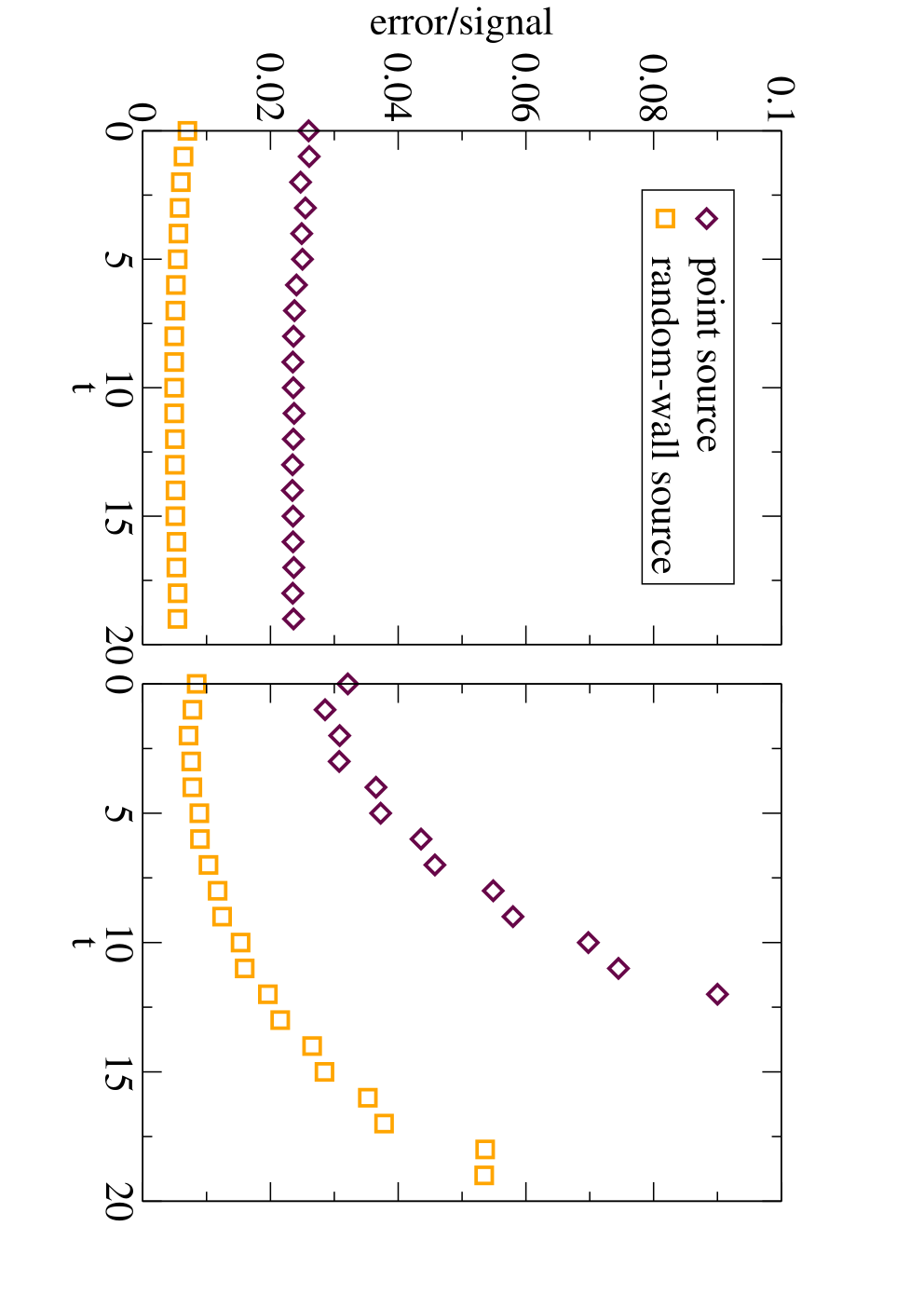
In Fig. 4 we show comparisons of percentage errors in three-point correlator data of local sources versus random wall sources. One sees significant improvement coming from random wall sources. These tests were carried out in the test case $D_{s}\rightarrow\eta_{s},l\nu$ calculations and with less than the full statistics. For $D\rightarrow K,l\nu$ we immediately went to random wall sources.

In addition to the three-point correlators, as we will show in the next section, several two-point correlators are needed in order to extract the matrix element $\langle K|S|D\rangle$. They are,

and

The $\frac{1}{L^{3}}\sum_{\vec{x}}$ can again be implemented via random wall sources. As already mentioned in the previous section we also calculated correlators for the $\eta_{c}$, $\eta_{s}$ and $D_{s}$ mesons in exactly the same way as $C^{2pnt}_{D/K}$ in order to carry out and check mass tunings. We have accumulated simulation data for the three- and two-point correlators described in this section for the ensembles of Table 1. In the next section we explain how hadronic matrix elements such as $\langle K|S|D\rangle$ and meson masses and decay constants are extracted from this data.

The interpolating operators $\Phi_{D}$ and $\Phi_{K}$ do not create just the ground state $D$ meson or kaon that we are interested in but also excited states with the same quantum numbers. With staggered quarks there is the further complication that in addition to regular states so-called “parity partner” states can contribute, whose energies are measured relative to $i\pi$ so that $e^{-Et}\rightarrow(-1)^{t}e^{-Et}$. The $D$ meson correlator, for instance, has the $t$ dependence (we set $t_{0}=0$ for simplicity),

We are interested in the ground state $D$ meson contribution with amplitude,

Similar relations apply for other mesons. Only in the case of equal mass mesons ($\pi$, $\eta_{s}$ or $\eta_{c}$) at zero momentum are the oscillatory contributions absent. The three-point correlators such as eq.(19) will have contributions from regular and oscillatory states for both the kaon and the $D$ meson. The rather complicated $t$ and $T$ dependence is then given by,

We will only consider the region $0\leq t\leq T$ and take $T<<N_{t}$ so that any contributions from mesons propagating “around the lattice” due to periodic boundary conditions in time can be neglected. The relevant amplitude here is,

From eqs.(23) and (5) one sees that our sought after hadronic matrix element is given by,

So our goal is to extract the combination on the right-hand-side of (26) as accurately as possible and with any correlations among the errors of the individual components, $A_{00}$, $b_{0}^{K/D}$, $M_{D}$ and $E_{K}$ taken properly into account.

We have carried out simultaneous fits to $C^{2pnt}_{D}$, $C^{2pnt}_{K}$ and the three-point correlators with different $T$ values, $C^{3pnt}(t,T_{i})$ $i=1,2...$. following the fit ansaetze of eqs.(V) and (V). Two (three) different $T$ values are used for the coarse (fine) ensembles. This allows us to evaluate (26) within one fit. The two-point correlators were fit for $t$-values between $t_{min}=2(2)$ and $t_{max}=30(20\sim 30)$ for the $K$ and $D$ respectively for coarse lattices. For fine lattices, $t$-values were used between $t_{min}=2\sim 4(2)$ and $t_{max}=30(30)$. For the three-point correlators we used all the data between $t=2$ and $t=T-2$ for coarse lattices, and $t=3$ and $t=T-2$ for fine lattices. Simultaneous fits with multiple $T$ and taking different fit ranges for different correlators were also helpful to reduce the statistical errors, since it allows us to extract maximum information from both the three-point and two-point correlators. The number of exponentials in our fit ansatz was varied to test for stability of fit results. For our final fits we ended up choosing around $3\sim 4$ for $N_{D}$ and $N_{K}$. $N_{D/K}^{\prime}$ was taken to be mostly $N_{D/K}-1$. Figs 5 - 9 show some results for $A_{00}$, $M_{D}$, $b^{D}_{0}$, $E_{K}$, $b^{K}_{0}$ versus $N_{D}$ or $N_{K}$ for ensemble C1 at kaon momentum $\vec{p}=(0,0,0)$. All our fits are carried out using Bayesian methods [21]. We describe choices for priors and prior widths in the Appendix.

We have found that using data from several $C^{3pnt}$ with different $T$-values helps greatly in reducing statistical/fitting errors. Fig. 10 compares results for $f_{0}(q^{2})$ for ensemble C2. One sees that having two rather than just one $C^{3pnt}(t,T_{i})$ involved in the simultaneous fit reduces errors and that this effect is most pronounced when one combines an even $T$ with an odd $T$. It may not be surprising that improvements are achieved from multi-T fits. From the fit ansatz (V) one sees that having more $C^{3pnt}$’s does not increase the number of fit parameters ($A_{jk}$ etc.) although the amount of data and hence of information given to the minimizer is increased. Furthermore if $T_{1}+T_{2}$ is odd, then $(-1)^{T_{1}-t}$ and $(-1)^{T_{2}-1}$ have opposite signs and $C^{3pnt}(t,T_{1})$ and $C^{3pnt}(t,T_{2})$ will provide more independent information.

Most of the fit parameters such as $M_{D}$ or $b_{0}^{D}$ etc. that one gets from the simultaneous $C^{2pnt}$ - $C^{3pnt}$ fits can also be determined by just fitting the two-point correlators by themselves. Results from the $C^{2pnt}$ fits are also shown on Figs. 6 - 9 and provide consistency checks. One interesting outcome is that two-point correlator parameters are more accurately determined via simultaneous fits with three-point correlators than when they are fit alone. This is especially noticeable for $D$ meson correlators, namely for $M_{D}$ and $b_{0}^{D}$ and has implications for determinations of the decay constant $f_{D}$. The latter is related to $b_{0}^{D}$ through,

In Figs. 11 and 12 we compare results for $M_{D}$ and $f_{D}$ using either pure two-point fits or simultaneous fits. One sees the significant improvement coming from the simultaneous fit. Doing simultaneous fits gives a better handle on excited state contributions because they contribute differently to two-point and three-point correlators. This is effectively similar to adding smearings to the correlators. In section VIII we will discuss extracting $f_{D}$ in the chiral/continuum limit. Having simultaneous fit results will make this determination more accurate than what can be achieved from pure two-point correlators. This appears to be a bonus side product of semileptonic decay studies.

In Tables 3, 4 and 5 we summarize our main fit results. One sees from Table 5 that we were able to determine $f_{0}(\vec{p}_{K})$ with errors ranging from $\sim 0.2$% at zero momentum to $\sim 0.9$% at our highest momentum. In Fig. 13 we plot the square of the “speed of light” $c^{2}(\vec{p})$ for the kaon.

One sees that the relativistic dispersion relation is satisfied to about $1\sim 2$%. We will check the effect of deviations from exact continuum dispersion relations on our final results for form factors in later sections.

References

- [1] M.Antonelli et al., FlaviaNet Working Group on Kaon Decays; arXiv:1005.2323 [hep-ph].
- [2] K. Nakamura et al. (Particle Data Group), J. Phys. G 37, 075021 (2010)
- [3] L.Widhalm et al. [Belle Collaboration]; Phys. Rev. Lett. 97:061804 (2006).
- [4]
B.Aubert et al. [BABAR Collaboration];
Phys. Rev. D76:052005 (2007),
BABAR update 2010; P.Roudeau private communication. - [5] D.Besson et al. [CLEO Collaboration]; Phys. Rev. D80:032005 (2009).
- [6] C.Aubin et al. [Fermilab Lattice, MILC and HPQCD Collaborations]; Phys. Rev. Lett. 94:011601 (2005).
- [7]
J.Bailey et al. [Fermilab Lattice and MILC Collaborations];
arXiv:0912.0214 [hep-lat],
E.Gámiz et al.; talk presented at LAT2010. - [8] E.Follana et al. [HPQCD Collaboration]; Phys. Rev. D75:054502 (2007).
- [9] S.Simula et al. [ETM Collaboration]; arXiv:0910.4845 [hep-lat].
- [10] E.Follana et al. [HPQCD Collaboration]; Phys. Rev. Lett. 100:062002 (2008).
- [11] H.Na et al. [HPQCD Collaboration]; arXiv:0910.3919 [hep-lat].
- [12] A.Bazavov et al. [MILC Collaboration]; arXiv:0903.3598 [hep-lat].
- [13]
C.G.Boyd, B.Grinstein and R.F.Lebed;
Phys. Rev. Lett. 74, 4603 (1995),
L.Lellouch, Nucl.Phys. B479, 353 (1996). - [14] M.C.Arnesen et al.; Phys. Rev. Lett. 95:071802 (2005).
- [15] T.Becher and R.J.Hill; Phys.Lett. B633, 61 (2006).
- [16] D.Becirevic, S.Prelovsek and J.Zupan; Phys. Rev. D68:074003 (2003).
- [17] C.Aubin and C.Bernard; Phys. Rev. D76:014002 (2007).
- [18] S.Naik, Nucl. Phys. B316, 238 (1989); G.P.Lepage, Phys. Rev. D59, 074502 (1999); K.Orginos et al., ibid. 60, 054503 (1999); C.Bernard et al., ibid. 61, 111502 (2000).
- [19] C.T.H.Davies et al. [HPQCD Collaboration]; Phys. Rev. D81:034506 (2010).
- [20] C.T.H.Davies et al. [HPQCD Collaboration]; arXiv:1008.4018 [hep-lat].
- [21] G.P.Lepage et al. [HPQCD Collaboration]; Nucl. Phys. B (Proc. Suppl.)106, 12 (2002).
- [22] C.Aubin et al. [MILC Collaboration]; Phys. Rev. D70:114501 (2004).
- [23] C.T.H.Davies et al. [HPQCD Collaboration]; Phys. Rev. D78:114507 (2008).
- [24] C.Amsler et al. Review of Particle Physics, Phys. Lett. B667:1, 2008.
- [25] A. Khodjamirian et al. Phys. Rev. D80:114005 (2009).
- [26] Heavy Flavor Averaging Group, http://www.slac.stanford.edu/xorg/hfag/charm/index.html .