Spectrum Shaping via Network Coding in Cognitive Radio NetworksThanks: This material is based upon work supported by the Air Force Office of Scientific Research under Contracts FA9550-09-C-0155 and FA9550-10-C-0026. Any opinions, findings and conclusions or recommendations expressed in this material are those of the authors and do not necessarily reflect the views of the Air Force Office of Scientific Research.
Abstract
We consider a cognitive radio network where primary users (PUs) employ network coding for data transmissions. We view network coding as a spectrum shaper, in the sense that it increases spectrum availability to secondary users (SUs) and offers more structure of spectrum holes that improves the predictability of the primary spectrum. With this spectrum shaping effect of network coding, each SU can carry out adaptive channel sensing by dynamically updating the list of the PU channels predicted to be idle while giving priority to these channels when sensing. This dynamic spectrum access approach with network coding improves how SUs detect and utilize temporal spectrum holes over PU channels. Our results show that compared to the existing approaches based on retransmission, both PUs and SUs can achieve higher stable throughput, thanks to the spectrum shaping effect of network coding.
Index Terms:
Cognitive radio networks; spectrum shaping; network coding; dynamic spectrum access.I Introduction
With the surge of a wide variety of wireless devices, the traditional static spectrum allocation poses an obstacle for efficient utilization of the limited spectrum resources. It is difficult for new users to find communication opportunities whereas the existing licensed or primary users (PUs) barely utilize the allocated spectrum to its full potential. According to the FCC measurement, only - on average has been used overall [1]. Such “virtual scarcity” in spectrum utilization has spurred a wealth of interest in studying cognitive radio (CR) that provides secondary users (SUs) with the capability of dynamically adapting physical layer characteristics to the available spectrum resources, thus enabling opportunistic access to the primary spectrum [2].
Cognitive radio goes beyond the conventional understanding of fixed network resource allocation and enables the coexistence of multiple user classes with varying priorities in a dynamic and hierarchical spectrum sharing environment. Hence, it is important for the SUs to capture temporal and spatial “spectrum holes” on PU channels, thereby enabling opportunistic spectrum access. One grand challenge in the design of CR networks is to discover spectrum holes for SUs and distribute them efficiently in heavily-loaded systems. In particular, a key functionality needed is the capability of sensing the spectrum and opportunistically accessing it without causing interference to the PUs. Spectrum holes appear in different ways, over space, time, and frequency. Particularly, the traffic pattern of the PUs directly determines the temporal spectrum availability and possibly leaves room for SU transmissions whenever PUs do not have any packet traffic to transmit.
In this paper, we consider a CR network with multiple PU channels, each representing a PU subnetwork. Within each subnetwork, PU packets are generated according to a stationary stochastic process. A base station (BS) over the PU channel buffers randomly arrived packets in its queue and multicasts them to a set of receiving PU nodes over lossy wireless channels. As expected, PU channels are not necessarily always busy and can be underutilized depending on packet arrival and link rates. With this observation, we analyze how SUs can discover these temporal spectrum holes (due to random packet traffic and random channel conditions) by trading channel sensing with data transmissions in a dynamic spectrum access environment.
Since SUs transmit on PU channels at idle instances of PUs, from a holistic perspective it is important to increase the transmission rates of PUs for given arrival rates, in order to enhance the spectrum access opportunities of SUs. However, the random nature of packet arrivals leads to stochastic and sporadic transmission patterns over the PU channels and “hides” the temporal spectrum holes from the SUs. We believe that it is beneficial to introduce some tangible structure into PU transmissions in the multicast setting with lossy communication links. To this end, we leverage network coding applied at PU channels to extend spectrum holes for SUs, as well as to make them more predictable to the SUs, i.e., network coding is used as a spectrum shaper on PU traffic.
Network coding is a novel networking paradigm that transforms the classical store-and-forward based routing. By allowing intermediate nodes to code over the incoming packet traffic, it is possible to improve the achievable throughput to the min-cut capacity for general multicast communications [3]. This coding diversity can be optimally realized by linear network coding [4], and distributed implementation is possible through random linear network coding (RLNC) [5] that improves the maximum flow rate to the min-cut capacity with high probability. The throughput benefits of network coding are not only possible in multi-hop operation but also apply to single-hop broadcast channels [6, 7, 8, 9] under both backlogged and stochastic packet traffic. Therefore, we can utilize network coding to improve PUs’ throughput rates, thereby extending temporal spectrum resources for SUs.
Beyond this apparent throughput gain for PUs (and extension of spectrum availability to SUs), we note that network coding further introduces a predictive structure associated with PU transmissions. Since PUs need to buffer batches of packets before coding them, their transmissions become more predictable and therefore make it easier for the SUs to discover the spectrum holes, whenever PUs become idle. This use of network coding here is similar in spirit to traffic shaping (e.g., leaky bucket [10]). Simply put, traffic shapers buffer the incoming data and retransmit them over time. The outgoing traffic resulted from the shaper is smoother and more regular at the expense of additional delay involved through buffering process. The same effect can be realized by network coding while boosting the throughput of both PUs and SUs in CR networks (without sacrificing delay performance in stable operation), and this is the main focus of our study.
We formulate a spectrum shaping framework where each BS over a PU channel first accumulates randomly arrived packets in its buffer and then applies RLNC to combine them before multicasting the coded packets to the receivers. Intuitively, when PUs use network coding, the busy periods on each of the PU channels are lower-bounded by the batch size of packets, and the idle periods are shaped based on the process of accumulating the packets. Transitions between the idle and busy periods become less frequent and more predictable due to the buffering of packets and their batch-based transmissions. Therefore, network coding applied by PUs reduces the need for channel sensing and creates more space for SUs’ data transmissions, thereby improving SUs’ throughput via the spectrum shaping effect, compared to ARQ-based retransmission schemes.
We propose an adaptive channel sensing scheme where the SU sets a timer for each PU channel that is sensed to be busy and does not revisit it for a period of time. In this way, the SU tracks a candidate list (we call this “sensing list” in subsequent sections) of possibly idle PU channels and performs a two-stage channel sensing: first, the SU senses the channels in the candidate list (with each of them being chosen randomly and sensed until an idle channel is detected) and then continues with the rest of the PU channels, provided that the candidate list does not include any idle channel. The timers for the PU channels form Markov chains that are coupled through the sensing list size. We characterize the candidate list evolution and compare the resulting throughput with random channel sensing (which is carried out independently of the sensing history). Significant throughput gains are attainable over ARQ when the PUs apply network coding and the SU performs random channel sensing. Further throughput gain is achieved when the SU performs the two-stage adaptive channel sensing supported by network coding over PU channels.
Our main contributions are three-fold:
- 1.
We propose to leverage network coding as a spectrum shaper in a CR network, aiming to enhance the spectrum discovery for SUs.
- 2.
We show that with network coding applied over PU channels only, both PU and SU’s throughput are increased, compared to the case when ARQ-based retransmission schemes are used by the PUs.
- 3.
We develop different sensing strategies for the SUs, and characterize the throughput attainable under random traffic, by balancing the tradeoffs between channel sensing and data transmissions for efficient spectrum access. The analysis is validated by simulation results.
In related work on spectrum sensing, much work has been carried out on exploiting the geographic and temporal properties of the signal power (e.g., energy, cyclostationary signal characteristics, interference and so on). Supportable communication regions, under which the SUs can safely transmit without interfering with the PU transmissions, were examined [11, 12, 13, 14, 15, 16, 17, 18, 19]. In reactive spectrum sensing, the SUs first sense the PU channels to detect the existence of PUs, and then decide whether to transmit or not based on the detection result [20]. In proactive spectrum sensing, the SUs predict future spectrum availability by exploring the history of spectrum usage and switch to a different channel expected to be available [21]. Our proposed method is a synergy of these two approaches, in the sense that the SU senses PU channels before transmission and prioritizes a candidate list of PU channels that are expected to be idle, and starts sensing from this candidate list. At the MAC-layer, a partially observable Markov decision process (POMDP) was used in [22] to model SUs’ sensing process and to search for the optimal sensing order. Also, a Markov decision process (MDP) framework was applied in, e.g., [23, 24], to determine the optimal sensing policy. Further, sensing period optimization was also studied (see e.g.,[25]).
Most existing studies focused on SUs’ performance, while little special attention was paid to the holistic performance improvement of both PUs and SUs. In contrast, our work here utilizes network coding as a spectrum shaper to create a more predictable structure of the spectrum holes, which simultaneously improves the throughput performance of both PUs and SUs.
The rest of the paper is organized as follows. Section II describes the system model, wherein a brief summary of PU’s stable throughput analysis is provided in Section II-B, for the two cases when PUs employ either ARQ or network coding. In Section III, we introduce the notion of spectrum shaping via network coding and develop two (random and adaptive) channel sensing schemes. Detailed analysis on random channel sensing is provided in Section IV, while Section V extends the study to adaptive channel sensing. In Section VI, SU’s throughput gains when network coding is used by the PUs are evaluated. In particular, the gain of adaptive channel sensing over random channel sensing is demonstrated. Finally we conclude the paper in Section VII.
II System Model & Background
II-A System Model
We consider a CR network consisting of PU channels. We focus on characterizing the spectrum shaping effect of network coding, in terms of the structural properties of PU spectrum holes, and developing efficient methods for SUs to discover and utilize the available spectrum resources. For ease of exposition, in our study here we consider one SU only (and the analysis readily extends to multiple SUs, each independently discovering spectrum holes on PU channels). Once PU spectrum holes are identified, the next step of coordinating SU transmissions can be handled separately depending on the choice of the medium access control mechanism, which we leave as a future design objective.
In this study, we assume that each PU channel is associated with a PU subnetwork consisting of one PU base station (BS) and receiving PU nodes (as shown in Fig. 1). Within each PU subnetwork, the BS multicasts data packets to the receiving nodes. We assume that the time is slotted and synchronized among PU channels. In each slot, packets arrive at any PU channel, , according to a stationary arrival process with a common rate . PU channels are lossy, with erasure probability . We assume independent erasures across channels and time slots. For ease of exposition, we consider this homogeneous CR network model, although the study can be carried over to general packet arrival models and channel erasure rates.

We assume that the transmission is carried out using either network coding or ARQ. If network coding is used, each BS accumulates a batch of packets, encodes them using random linear network coding, and multicasts the coded packets to the receivers. Once all receivers of a PU subnetwork decode the entire batch of packets, the BS proceeds with the next batch of packets, provided that there are enough buffered packets. If not, the PU BS waits to accumulate the next batch of packets. Random linear network coding is carried out in the Galois field , where is the finite field size. We assume a large value of so that with high probability (as specified in [5]), each generated coded packet would be innovative and each receiver simply needs to receive exactly coded packets in order to decode the whole batch of packets.
In contrast, if ARQ is used by the PUs, each BS multicasts individual packets one by one. The BS keeps retransmitting each packet (in uncoded plain form) until all receivers successfully receive it. Then, the BS proceeds with transmitting the next packet in the buffer.

As is standard, the SU opportunistically explores spectrum holes on PU channels for data transmissions. We assume synchronization across the SU and PUs. The packet transmission of a PU continues one slot (or time frame) and each slot of the SU amounts to mini-slots, which are used either for sensing different PU channels or transmitting packets. Clearly, at most channels can be sensed per slot, i.e., the SU would be able to sense all PU channels when needed only if . Sensing is performed based on the “sensing list” in every slot , which consists of the channels that are considered by the SU as “possibly idle” in this slot. When sensing, the SU picks a channel randomly and uniformly from the list at a time without replacement. After channel sensing, the SU transmits data packets during the rest of the time slot, provided that an idle channel is detected; otherwise, the SU waits till the next slot and repeats the procedure. Fig. 2 illustrates the slot structure, where points to the end of the sensing phase whenever the SU decides to transmit.
It is clear that when PUs use network coding, the transmission is performed on a batch basis with size . On the other hand, when ARQ is used by the PUs, the transmission is carried out per individual packet. This major difference implies that network coding not only extends the possible spectrum hole but also makes the spectrum structure more “regular,” namely, easier for SUs to predict when it is idle. With this insight, we should expect that the SU keeps a shorter sensing list when PUs use network coding compared to the case when ARQ is used. More specifically, when PUs use network coding, we have
| (1) |
and when PUs use ARQ,
| (2) |
where is the size of the sensing list. In particular, the sensing list size can be updated dynamically, when network coding is used, and we will show in Section VI that this results in higher throughput beyond random channel sensing. In the sequel, we will analyze different strategies taken by the SU for channel sensing, for cases when PUs use ARQ or network coding. Before that, we briefly demonstrate the gain brought by network coding over the PU channels in the following.
II-B PU’s Throughput and Idle Probability
For broadcast erasure channels, it is well-known that network coding reduces the completion time of data transmission compared to retransmission schemes [6], [9]. For completeness, we characterize the stable throughput and busy/idle periods of PUs for both cases when PUs use network coding and ARQ in the following.
II-B1 When PUs use network coding
Random network coding with large ensures that each of the PU receivers can decode the original packets with high probability, as long as it receives exactly coded packets [5]. Let denote the completion time for all receivers to successfully decode packets. Based on [6], the expected time is given by
The stability condition of the PU queues is given by , where the maximum stable throughput is
| (4) |
From Little’s theorem [26], the idle probability of each PU BS can be obtained as
| (5) |
II-B2 When PUs use ARQ
For ARQ, the completion time of any individual packet is the number of time slots necessary for successful reception of it at all receivers. Let denote this time. Note that ARQ is equivalent to network coding with batch size . From (II-B1) with , the expected service time is obtained as
| (6) |
The stability condition of the PU queues is given by , where the maximum stable throughput is
| (7) |
It follows that the idle probability of the PU channels is
| (8) |
As a result, we have and therefore
| (9) |
As expected, network coding increases the stable throughput for PUs and provides the SU with extended availability of the primary spectrum. Beyond this throughput gain, as we show in the subsequent sections, network coding also shapes the spectrum and increases the predictability of whether PU channels are idle or not, which in turn reduces the channel sensing time by the SU, thus further improving the SU’s throughput.
III Spectrum Shaping via Network Coding
We start this section with a special case with a single PU channel, and illustrate the basic idea of spectrum shaping. We then turn to the general multi-channel scenario, which is the main focus of the analysis in the sequel.
III-A The Case with a Single PU Channel
When there is a single PU channel, the SU is able to track the dynamics on the channel continuously by sensing it every slot. Intuitively, such a strategy is plausible if the PU uses ARQ-based transmission mechanism, since the packet arrivals are random and the transmission is carried out on a per packet basis. Then, the SU senses the channel using the first mini-slot in every slot, and after sensing, if the channel is sensed to be busy, the SU backs off and senses it again.
However, when network coding is used by the PU, the spectrum is better “shaped” in the sense that the transmission period becomes more regular and is bounded below by the batch size . Consequently, it is not necessary for the SU to sense the channel every slot while not losing tractability on it. Instead, the SU simply backs off for slots when the channel is sensed to be busy, and starts sensing every slot after slots. Clearly, the SU is able to recognize the starting time slot for every transmission period after it finds the channel idle in the first place. Therefore, such a backoff scheme is accurate in predicting the minimum completion time (i.e., ) while preventing the SU from missing any potential spectrum holes, and this reduces the sensing overhead without sacrificing the SU’s throughput, compared to the case when the PU uses ARQ.
III-B The Case with Multiple PU Channels
When there are channels in the CR network, the SU is no longer capable of keeping track of each channel all the time. The SU either senses a subset of them before transmitting, or gives up channel sensing for the current time slot (if none of the channels can be idle). Intuitively speaking, the SU needs to find an idle channel as soon as possible, while keeping the sensing cost low by exploiting the underlying traffic structure. When ARQ is used by the PUs, the PU channels experience fast idle-busy alternations on a per slot basis. However, when network coding is used by the PUs, the transitions between the idle and busy states would become slower on the scale of slots. Therefore, if network coding is used by the PUs, the SU would be better off by adaptively updating the sensing list. Based on the relationship of the time spent for channel sensing, namely sensing cost, and the achievable throughput, the SU can take different strategies for updating the sensing list.
We develop the following two strategies for the SU:
- •
Random channel sensing under network coding and ARQ. In every slot, the SU picks one channel randomly and uniformly from the complete list (i.e., the list with all channels) and senses it. If the channel is busy, the SU chooses another channel randomly and uniformly in the next mini-slot and senses it. If the channel is busy, the SU continues. Otherwise, the SU stops at the channel and transmits on it using the rest of the slot. Loosely speaking, random channel selection is more appropriate for ARQ, since the alternations between idle and busy states are fast. Nevertheless, as we show later, when PUs apply network coding, the SU’s throughput can be significantly improved, compared to the case when ARQ is used.
- •
Backoff-based adaptive sensing under network coding.
As pointed out before, when network coding is used by PUs, the SU can predict “slower” transitions between PUs’ idle and busy states due to additional buffering and batch transmissions of coded packets. Instead of keeping all channels in the sensing list, the SU seeks for a shortened list while hoping to reduce the time it takes to find an idle channel. In each time slot, the SU carries out a two-stage sensing. First, the SU starts sensing PU channels randomly picked from the sensing list one by one, and stops whenever an idle PU channel is detected. In the meantime, SU backs off on channels sensed to be busy for slots and updates the list based on the channel sensing information. The SU sets a timer for each PU channel it backs off and moves the particular channel back to the candidate sensing list only after slots.
If all channels in the first stage are found to be busy, the SU proceeds to the second stage and randomly searches for an idle channel in the backup list , namely the list of channels excluding , with size , until it finds one.11 1 Note that the sensing capability can be further improved by ordering channels in the back-up list according to their timer values and giving priority to those channels with smaller timer values in the sensing order. However, this would increase the complexity significantly. Instead, we consider random channel selection from the backup list in the second stage. In this stage, the SU moves the channel that it senses idle back to the sensing list, but does not change the timers of channels that are detected to be busy.
The intuition behind this two-stage sensing approach is to give higher sensing priority in the first stage to channels that are more likely to be idle while seeking for an idle channel beyond the priority list, if necessary. The backoff parameter can be expressed as a function of the batch size , namely . Without prior information (i.e., when the SU visits a busy channel for the first time), on average the SU would find the PU transmissions in the middle of the batch service time. Therefore, we can intuitively let , with given in (II-B1). For any channel, the SU should choose as the backoff timer the average remaining time it believes for the PU to complete the transmission of the current batch. We will evaluate the effects of on the channel sensing and throughput performance in Sections V and VI.
III-C SU’s Throughput
Let represent the number of mini-slots used for sensing in slot by the SU. Define a “good slot” to be one in which the SU finds an idle channel and transmits. Correspondingly, a slot is called “bad” if the SU fails in obtaining any transmission opportunity therein. Let be the indicator random variable indicating whether slot is good () or bad (). Since the SU can transmit data packets only over mini-slots (whenever SU does not sense the channels) and only if the channel sensing is successful (i.e., only if it detects one idle PU channel), the SU’s throughput can be obtained as
| (10) | |||||
where is the time period under observation, , and (10) follows from the ergodicity of the channel sensing process.
In the following, we focus on multiple PU channels and show how network coding enables new opportunities for dynamic spectrum sensing and improves the SU’s throughput compared to ARQ, while reducing the sensing cost.
IV Random Channel Sensing
When the SU uses random channel sensing, it probes the channels one by one randomly in each slot, until it finds an idle channel.
IV-A When PUs use Network Coding
Note that the SU cannot sense all channels when is smaller than (even though it keeps the sensing list size unchanged as ). Accordingly, we study two cases in the sequel: and .
When , i.e., when the slot length can accommodate sensing all channels, the probability that there exists at least one idle PU channel is
| (11) |
and, if an idle channel exists, the number of mini-slots used for sensing is
| (12) |
for . Based on (10), the throughput of the SU can be derived as
| (13) | |||||
On the other hand, when , we shall consider only the first slots. Correspondingly, we have
| (14) | |||||
| (15) |
for . In this case, the SU’s throughput is given as
| (16) | |||||
IV-B When PUs use ARQ
Similarly, we consider two regions as in the previous case. When , we have
for .
It follows that the SU’s throughput is
| (17) | |||||
On the other hand, when , the throughput of the SU can be obtained as
| (18) | |||||
V Backoff-based Adaptive Sensing
V-A The Case with
We start with the case . In adaptive sensing, the SU dynamically updates the size of the sensing list based on the sensing results from the current slot. It follows that the sensing list size, , becomes a random variable in itself in this case. For notational convenience, denote . To quantify the SU’s throughput, we consider two stages: sensing within the sensing list and beyond it within the backup list . Define (respectively ) as the indicator function indicating whether there exists at least one idle channel in the first (respectively second) stage. Clearly, only if the SU fails in the first stage, i.e., all channels in the sensing list are found to be busy, the SU will proceed into the second stage. Accordingly, can be obtained as the same in (11), and the number of mini-slots used for finding an idle channel, provided that there exists at least one idle PU channel, is computed as
| (19) | |||||
The calculation of SU’s throughput then follows from (10). However, it is observed that in order to characterize the SU’s throughput, we shall first characterize , the distribution of . Note that once a PU channel is sensed to be busy, the SU backs off on this channel by setting up a countdown timer with an initial value . The evolution of such a timer follows a Markov chain, where states correspond to the countdown values of the timer, or equivalently, the remaining time slots before the channel is moved back to the sensing list . It is noted that the value of the timer decreases from to at a rate of per slot. When it enters state , the corresponding channel is considered as a potential candidate in the sensing list again, and it remains in the list as long as it is sensed to be idle or it is simply not sensed. On the contrary, the channel is removed from the sensing list in the next slot, provided that it is sensed to be busy. In the meanwhile, if the SU enters the second stage and senses the channels therein, the state of the idle channel it finally finds changes to 0 in the next slot. Thereby, the Markov chain for the timer should include transitions from states to state , as depicted in Fig. 3. Accordingly, the transition probabilities can be expressed as
| (20) |
where is the probability that a PU channel in the sensing list is sensed in the first stage, and represents the probability that a PU channel in the backup list is sensed provided that all channels in the sensing list are found busy.

Recall that the PU channels in both lists are randomly chosen and sensed, until an idle channel is detected. The Markov chains of timers for different PU channels are coupled with each other through the size of the sensing list , which in turn depends on the states of the individual Markov chains, namely how many of them are in state . An approximation is necessary to integrate the effects of all PU channels (similar approach has been taken in e.g., [27], to analyze IEEE 802.11 backoff mechanism). In particular, we average the sensing probability of the first stage, , and obtain that
| (21) |
Along the same line, the sensing probability of the second stage, , can be characterized as
| (22) | |||||
where .
The stationary distribution for the states in the Markov chain is given by
| (23) |
Based on (20)-(23), , the probability that any given PU channel is in the sensing list , can be computed as
| (24) |
It follows that the size of the sensing list, , has a binomial distribution with parameter , i.e., is expressed as
| (25) |
Let . We note that (25) consists of a fixed point equation of form for p. Since is a continuous mapping on a compact space, there exists a solution to . Furthermore, p consists of the stationary distributions of the positive recurrent Markov chain that represents the overall PU channel states (it has a finite number of states and it is commutative), it follows that there exists a unique solution to (25).
V-B The Case with
V-C Prediction Accuracy of Spectrum Opportunities
In the backoff-based sensing strategy, the SU predicts the spectrum holes by adaptively updating the sensing list. As can be noted from the analysis above, the calculation of SU’s throughput heavily hinges on the distribution of the sensing list size, , where the key parameter is the idle probability of the PU channels. Clearly, in the actual underlying system, this probability is given by , while in the predicted system built from the adaptive sensing strategy, the expected idle probability on the PU channels is given by (24). In order to examine the prediction accuracy, we define the following distance to quantify the difference between the two:
| (29) |
Intuitively, the smaller the distance , the more accurate the prediction is. To get a more concrete sense, we plot in Fig. 4 and 5 some examples on the comparison of and , where we set and as the default values. As can be seen from Fig. 4, the prediction closely tracks the idle probability of the actual system for different erasure probabilities , indicating the robustness of channel tracking against channel variations. On the other side, as Fig. 5 demonstrates, when the backoff parameter increases, the difference first sharply shrinks and then increases slowly after reaches a certain value. This points to an optimal backoff parameter:
| (30) |
for capturing the spectrum holes. Intuitively, if is chosen to be smaller than the optimal one, the sensing list would be longer than necessary with redundant PU channels that are actually busy. On the other hand, if is greater than (30), the SU tends to perform a conservative sensing policy with a shorter list of candidate channels to be sensed.


VI Performance Evaluation
In this section, we illustrate, via numerical examples, the throughput gain of the SU when PUs use network coding. Fig. 6 and 7 show that compared to ARQ, the SU’s throughput is greatly increased when PUs use network coding and the SU employs random channel sensing. Clearly, with variations in the parameters, and , the SU’s throughput improves with network coding, for both cases with and . Besides, as the values of these parameters increase, the gain also increases.
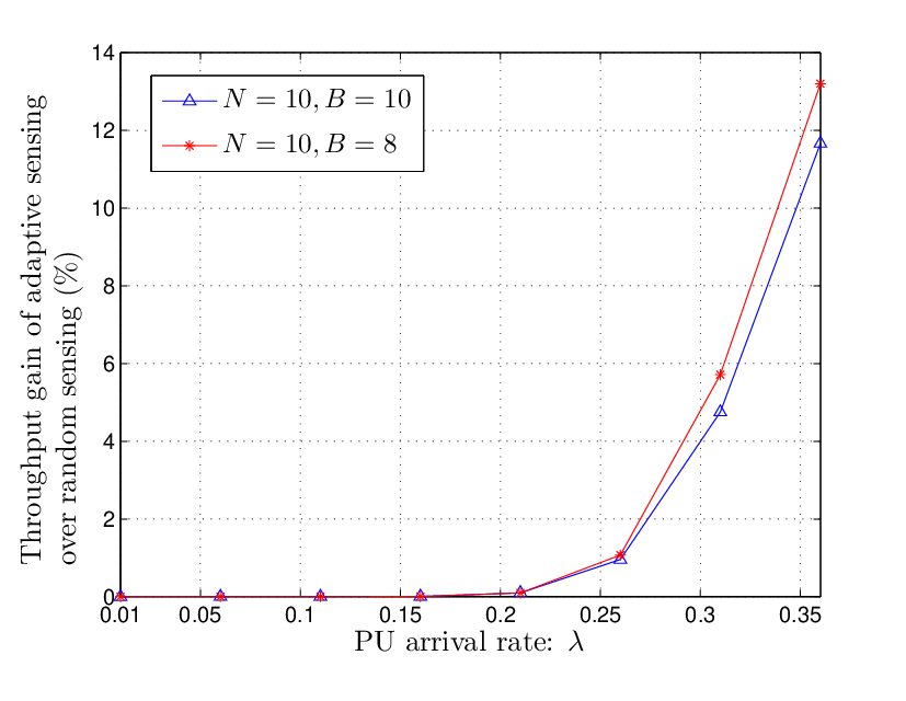
Next, we show that by employing the adaptive sensing strategy, the SU’s throughput can be further improved by almost , as Figs. 8-11 indicate, where the default values of parameters are and . The two-stage adaptive sensing strategy provides further gain over the random sensing mechanism, over the entire region of parameter variations (in , , , and ). Fig. 8 and 9 show that the gain increases with the PU arrival rate and channel erasure probability, and as illustrated in Fig. 10, the gain strongly depends on the network coding batch size as well. Moreover, Fig. 11 shows that the backoff parameter can be further adjusted by the SU to improve the gain of adaptive sensing.
We have a few more remarks on the above results. As either or increases, the idle probability of the PU channels decreases and the adaptive sensing scheme, in which the SU makes more use of system information, reveals more gain over the random sensing scheme, where dominates the performance. Differently, if increases, the service rate of the PUs increases to the min-cut capacity given by [6]. This increases the idle probability of the PU channels for fixed arrival rates and shrinks the operational difference between the random and adaptive sensing strategies. Finally, we observe that optimizing over the backoff parameter improves the performance of the adaptive sensing strategy, as has also been observed in Section V-C. On one hand, we have for , i.e., the random sensing strategy serves as a special case of the adaptive sensing scheme for . On the other hand, as increases, almost all PU channels are included in the backup list and the adaptive sensing strategy performs again closely to the random sensing scheme. Therefore, we expect an optimal with an intermediate value to yield the highest performance gain.




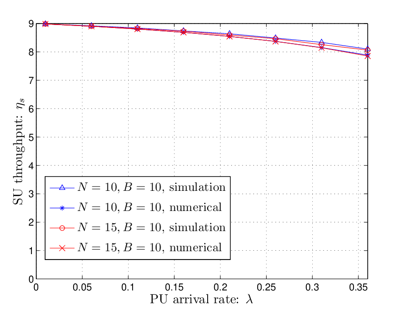
Finally, we take a closer look at the adaptive sensing scheme. As pointed out in Section V-A, we approximate the sensing probabilities and in the Markov chain analysis and compute the SU’s throughput accordingly. To validate this approximation, we perform Monte Carlo simulations over trials and compare them with the numerical evaluation of the analysis in Figs. 12-15. The default parameters are and . As can be seen from the figures, the numerical results from the analysis match with simulations under variations in all parameters. On average, the maximum difference between the numerical and simulation results is less than , indicating that the approximation in the analysis of adaptive sensing performs closely to the real system implementation.


VII Conclusion
We considered a CR network with PU channels and one SU, where each PU transmits packets to multiple receivers over lossy wireless channels via ARQ or network coding. Viewing network coding as a spectrum shaper, we showed that it increases the spectrum availability for the SU and offers a more predictive structure to the PU spectrum, i.e. it improves the SU’s prediction of spectrum holes on PU channels. Based on the spectrum shaping effect of network coding, we developed different sensing strategies for the SU, where adaptive channel sensing is carried out by dynamically updating the list of the PU channels that are predicted by the SU to be idle. Our analysis and numerical results showed that compared to retransmission, both PU and SU’s throughput can be improved when PUs apply network coding instead of ARQ, and the SU can further improve this gain by applying adaptive channel sensing (based on sensing history to reflect the PU traffic).
Future work is needed to quantify the gain of dynamic spectrum access for other channel models and to integrate medium access control for multiple SUs applying dynamic channel sensing with network coding. In particular, it is of great interest to study multi-hop CR networks where network coding has potential to offer more opportunities for PUs to improve their throughput. We expect that our initial steps here open a new avenue for SUs to discover spatial and temporal spectrum holes via spectrum shaping effects of network coding.
References
- [1] “Report of the spectrum efficiency working group,” FCC Spectrum Policy Task Force, Tech. Rep., Nov. 2002.
- [2] J. Mitola III, “Cognitive radio: an integrated agent architecture for software defined radio,” Ph.D. dissertation, KTH Royal Institute of Technology, 2000.
- [3] R. Ahlswede, N. Cai, S.-Y. R. Li, and R. W. Yeung, “Network information flow,” IEEE Transaction on Information Theory, vol. 46, pp. 1004–1016, Jul. 2000.
- [4] S. Li, R. Yeung, and N. Cai, “Linear network coding,” IEEE Transaction on Information Theory, vol. 49, no. 2, pp. 371–381, Jul. 2003.
- [5] T. Ho, R. Koetter, M. Médard, M. Effros, J. Shi, and D. Karger, “A random linear network coding approach to multicast,” IEEE Transaction on Information Theory, vol. 52, no. 10, pp. 4413–4430, Oct. 2006.
- [6] A. Eryilmaz, A. Ozdaglar, and M. Mdard, “On the delay and throughput gains of coding in unreliable networks,” IEEE Transaction on Information Theory, vol. 54, no. 12, pp. 5511–5524, 2008.
- [7] D. Lucani, M. Médard, and M. Stojanovic, “Random linear network coding for time-division duplexing: queueing analysis,” in Proc. IEEE ISIT’09.
- [8] D. Nguyen, T. Tran, T. Nguyen, and B. Bose, “Wireless broadcast using network coding,” IEEE Transaction on Information Theory, vol. 58, no. 2, pp. 914–925, 2009.
- [9] Y. E. Sagduyu and A. Ephremides, “On broadcast stability of queue-based dynamic network coding over erasure channels,” IEEE Transaction on Information Theory, vol. 55, no. 12, pp. 5463–5478, 2009.
- [10] R. L. Cruz, “A calculus for network delay, part I: network elements in isolation,” IEEE Transaction on Information Theory, vol. 37, no. 1, pp. 114–131, 1991.
- [11] I. F. Akyildiz, W.-Y. Leea, M. C. Vuran, and S. Mohantya, “Next generation/dynamic spectrum access/cognitive radio wireless networks: A survey,” Computer Networks, vol. 50, no. 13, pp. 2127–2159, 2006.
- [12] S. Haykin, “Cognitive radio: brain-empowered wireless communications,” IEEE Journal on Selected Areas in Communications, Special Issue on Cognitive Networks (Invited), vol. 23, pp. 201–220, 2005.
- [13] L. Cao and H. Zheng, “Stable and efficient spectrum access in next generation dynamic spectrum networks,” in Proc. INFOCOM’08, 2008.
- [14] N. Chang and M. Liu, “Competitive analysis of opportunistic spectrum access strategies,” in Proc. INFOCOM’08, 2008.
- [15] Y. Chen, Q. Zhao, and A. Swami, “Joint design and separation principle for opportunistic spectrum access in the presence of sensing errors,” IEEE Transaction on Information Theory, vol. 54, no. 5, pp. 2053–2071, 2008.
- [16] Y. Hou, Y. Shi, and H. Sherali, “Optimal spectrum sharing for multi-hop software defined radio networks,” in Proc. INFOCOM’07, 2007.
- [17] S. Huang, X. Liu, and Z. Ding, “Opportunistic spectrum access in cognitive radio networks,” in Proc. INFOCOM’08, 2008.
- [18] R. Tandra, M. Mishra, and A. Sahai, “What is a spectrum hole and what does it take to recognize one?” IEEE special issue on Cognitive Radio, pp. 824–848, May 2009.
- [19] R. Urgaonkar and M. Neely, “Opportunistic scheduling with reliability guarantees in cognitive radio networks,” in Proc. INFOCOM’08, 2008.
- [20] S. Wang, J. Zhang, and L. Tong, “Delay analysis for cognitive radio networks with random access: a fluid queue view,” in Proc. INFOCOM’10, 2010, pp. 1055–1063.
- [21] L. Yang, L. Cao, and H. Zheng, “Proactive channel access in dynamic spectrum networks,” Elsevier Physical Communication, vol. 1, no. 2, pp. 103–111, Jun. 2008.
- [22] S. Ahmad, M. Liu, T. Javidi, Q. Zhao, and B. Krishnamachari, “Optimality of myopic sensing in multi-channel opportunistic access,” IEEE Transaction on Information Theory, vol. 55, no. 9, pp. 4040–4050, 2009.
- [23] N. B. Chang and M. Liu, “Optimal channel probing and transmission scheduling for opportunistic spectrum access,” in Proc. mobihoc’07, 2007.
- [24] H. Jiang, L. Lai, R. Fan, and H. V. Poor, “Optimal selection of channel sensing order in cognitive radio,” IEEE Transaction on wireless communications, vol. 8, no. 1, pp. 297–307, 2009.
- [25] H. Kim and K. G. Shin, “Efficient discovery of spectrum opportunities with MAC-layer sensing in cognitive radio networks,” IEEE Transaction on Mobile Computing, vol. 7, no. 5, pp. 533–545, May 2008.
- [26] D. Bertsekas and R. Gallager, Data Networks, 2nd Edition. Prentice Hall, 1992.
- [27] G. Bianchi, “Performance analysis of the IEEE 802.11 distributed coordination function,” IEEE Journal on Selected Areas in Communications, vol. 18, no. 3, pp. 535–547, 2000.
*