Dynamical model for the formation of patterned deposits at receding contact lines
Abstract
We describe the formation of deposition patterns that are observed in many different experiments where a three-phase contact line of a volatile nanoparticle suspension or polymer solution recedes. A dynamical model based on a long-wave approximation predicts the deposition of irregular and regular line patterns due to self-organised pinning-depinning cycles corresponding to a stick-slip motion of the contact line. We analyze how the line pattern properties depend on the evaporation rate and solute concentration.
pacs
68.15.+e, 47.57.-s, 81.15.Lm, 81.16.RfThe last decade has seen huge growth in interest in phenomena that accompany evaporative and convective dewetting of suspensions and solutions. Well known are the detailed studies of the coffee stain effect [1, 2] that analyse the deposition and resulting structures left behind by a receding three-phase contact line of an evaporating drop of suspension upon a solid substrate. In particular, Ref. [2] describes a large range of different deposition patterns including cellular and lamellar structures, single and multiple rings, and Sierpinski gaskets. Other observed structures include crack [3] and chevron [4] patterns. Recently it has been shown that evaporating polymer solutions [5, 6, 7] and (nano)particle suspensions [8, 9, 10] may be used to fabricate strikingly regular stripe patterns, where the deposited stripes are parallel to the receding contact line and have typical distances ranging from 10-100m. The goal is to use this effect as a non-lithographic technique for covering large areas with regular arrays of small-scale structures, such as, e.g., concentric gold rings with potential uses as resonators in advanced optical communications systems [11]. The deposited patterns from more complex fluids, such as polymer mixtures [12] and DNA solutions [13], are also investigated. The occurrence of regular stripe patterns is a somewhat generic phenomenon, that is not only observed for different combinations of substances but also in a variety of experimental setups that allow for slow evaporation. Examples include the meniscus technique in a sphere-on-flat geometry [9, 7], a controlled continuous supply of liquid between two sliding plates to maintain a meniscus-like surface [5] and dewetting forced by a pressure gradient [10]. Interestingly, besides the stripes parallel to the receding contact line, a variety of other patterns are observed, including regular orthogonal stripes [9], superpositions of orthogonal and parallel stripes [5], regular arrays of drops [14, 5] and irregularly branched structures [14, 15]. This behaviour is highly sensitive to the particular experimental setup and parameters.
Despite the extensive number and variety of experiments, an explanation of the formation of the regular patterns has been rather elusive. Although most studies agree that the patterns result from a stick-slip motion of the contact line caused by pinning/depinning events [2, 11, 6, 16] no dynamical model of the periodic deposition process exists. Most models assume a permanently pinned contact line (see [17, 18] and references therein) and are therefore only able to describe the formation of a single line deposit. A non-isothermal Navier-Stokes simulation shows depinning from such a single line but no periodic deposits [16]. The model of Ref. [19] describes drop arrays formed via directed dewetting of the solvent that are subsequently dried.
In this Letter we discuss a generic close-to-equilibrium model for the evaporative and convective receding of a three-phase contact line of a solution or suspension on a solid substrate. We show that solely having a viscosity that diverges at a critical solute concentration is sufficient to trigger a self-organised periodic pinning-depinning process that results in the deposition of regular line patterns. The model can easily be extended to incorporate other processes and in the future may be employed to assess their influence on the basic mechanism that we describe here.

We consider a thin film of an evaporating partially wetting nanoparticle suspension (or polymer solution) in contact with its vapour on a flat solid substrate (see Fig. 1). Assuming that all surface slopes are small, one may employ a long-wave approximation [20] and derive two coupled evolution equations for the film thickness profile and the vertically averaged solute concentration field :
| (1) | |||||
| (2) |
The mobility models Poiseuille flow and incorporates the dynamic viscosity that exhibits a strong non-linear dependence on the local solute concentration. We employ the Krieger-Dougherty law [21, 22]
| (3) |
where is the viscosity of the pure solvent. We have scaled by the concentration at random close packing () so that diverges when . The precise value of the exponent depends on the type of suspension. For non-interacting particles (i.e. particles that have no net attractive forces between them and only have excluded volume interactions), values for between 1.4 and 3 are discussed, depending on the shape of the particles [21]. For spherical particles the factor , giving . Other thin film models use [23, 19]. For interacting solute particles, values for as low as 0.13 are reported [24]. Depending on the particular system, the transition at is either referred to as jamming or gelation [24]. Here we fix , although we have found that the effects we describe below are even stronger for smaller .
The first term on the right hand side of Eq. (1) (conserved part) corresponds to convective transport of the liquid whereas the second term (non-conserved part) models evaporation. The convective flow is driven by the gradient of the pressure
| (4) |
where the first term is the Laplace pressure ( is the surface tension) and the second is the disjoining pressure that models a partially wetting fluid [25, 26]. Here, is the Debye length, is a molecular interaction length, and are the apolar and polar spreading coefficient, respectively, and is the Hamaker constant. To derive the second term in Eq. (1) we assume the system is close to equilibrium and near to saturation and so evaporation is slow. In this limit evaporation with a rate is driven by the difference of the scaled pressure and the chemical potential of the ambient vapour [27, 28]. Latent heat effects may be neglected, and the density is assumed to be equal for particles and solvent. The first and second terms on the right hand side of Eq. (2) model convective and diffusive transport of the particles, respectively. Note that the diffusion coefficient depends on concentration and we employ the Einstein-Stokes relation , where is the Boltzmann constant, the temperature, and the particle radius.
Models related to Eqs. (1) and (2) are used in studies of particle-laden film flow [23] (without evaporation or wettability effects) and dewetting of suspensions of surface active particles [19] (different wettability regime). In the limit , our theory reduces to that used in [27] to study the fingering instability of an evaporative front of a pure liquid. We choose our scaling and some of the parameters to be the same as in [27]: The dimensionless chemical potential and the diffusion number , where . Our main control parameters are the initial mean (dimensionless) concentration and the evaporation number which represents the ratio of the time scales for convection and evaporation of a film without solute. We solve the nondimensional model by discretizing over a spatial domain of finite length . Deposited patterns are obtained by direct time simulations using a variable-step variable-order backward difference scheme starting from an initially step-like front that becomes smooth in the early evolution [29].

In the evaporative dewetting process one encounters different types of receding fronts. In the case without solute [27] one may distinguish the limiting cases of (i) convection-dominated and (ii) evaporation-dominated dewetting for small and large values of , respectively. In case (i) the front recedes rapidly and convective motion maintains a capillary ridge despite evaporation. In case (ii) convection is much slower than evaporation, the front recedes slowly and there is no capillary ridge. In the presence of a solute the situation is more complex and stationary receding front shapes are not found for some parameter values. In general, on starting with a uniform concentration , as the front recedes, it deposits part of the solute in a smooth layer. Evaporation in the contact line region increases the local concentration and consequently also the viscosity. When , the convective motion in the contact region stops completely (the suspension becomes locally jammed) due to the strong non-linearity in Eq. (3). One may say that the initial convection-dominated stage changes into an evaporation-dominated regime as the local evaporation number becomes large. At this stage the front seems pinned. However, it is actually still moving extremely slowly, solely by evaporation, and deposits a first line of solute. During this, the local concentration in the contact region decreases, i.e., decreases, until the front depins and convective motion resumes. Subsequently, after the initial line is deposited, various scenarios are possible: (a) a deposit of uniform thickness (i.e. only a single line is deposited), (b) deposition of a finite number of lines followed by a layer of constant thickness, (c) intermittent line pattern, and (d) regular line pattern. In the narrow region of parameter space where the ‘limiting’ case (c) occurs, we find that this behaviour is normally very sensitive to computational details (which is not the case for (d)), so we believe that the intermittent line patterns represent a ‘chaotic deposition’. Typical profiles are displayed in Fig. 2 and the corresponding parameter ranges are marked in the phase diagram Fig. 3.
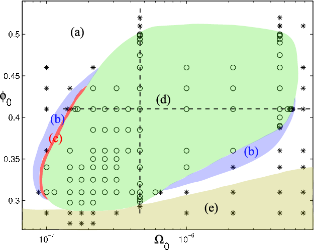
Ignoring initial transients, we distinguish two main types of deposits: those of uniform thickness (regions (a), (b) and (e) in Fig. 3) and periodic line patterns (region (d)). In the latter one observes (as in the experiments [11, 6, 10]) a regular stick-slip motion of the contact line, since the typical time scales for convection-dominated and evaporation-dominated front motion may differ by orders of magnitude.
Structure formation results from a subtle interplay between convection, evaporation, and diffusion. The basic mechanism of line deposition described above stems from a balance of convective and evaporative motion. Diffusion does not change that picture as long as its time scale is not much shorter than the convective and evaporative time scales. Increasing merely shrinks the region (d) in Fig. 3. However, in the unlikely situation that diffusion is so fast that nanoparticles diffuse away ahead of the receding contact line (e.g. when ), then line deposition is suppressed. We do not consider this case here.


Next, we analyse regular line patterns as obtained from long-time simulations [29]. Excluding the initial transient we take a sequence of regular deposition periods (lines), where , depending on the period of the deposit and required CPU time. We measure the amplitude, relative width (defined as , where is the standard deviation) and skewness of the lines, and the period of the line pattern. We find that these quantities strongly depend on both the evaporation number and the concentration . We focus on two cuts through region (d) in Fig. 3 (dashed lines).
First, we fix and vary the bulk concentration . Fig. 4 presents line characteristics and selected profiles. On increasing from a region without periodic line deposition, one first finds large amplitude almost solitary peaks separated by very large distances. On further increasing , the amplitude first hardly changes and later decreases. The period continuously decreases while the relative width increases. For higher the deposit pattern becomes almost uniform, with a small amplitude harmonic modulation. Finally, the amplitude goes to zero (at finite period) at the upper border of the region (d).


Second, Fig. 5 presents results for fixed and varying . Increasing , moving from the narrow region (b) of multiple lines (Fig. 3), one passes through a very narrow band of intermittent line patterns (c) followed by the region (d) of regular line patterns. For the lowest values of in (d), the patterns have a relatively small period and a small but non-zero amplitude. The strongly anharmonic peaks are skewed to the right with their tail pointing towards the receding front. On increasing the period increases. The amplitude, however, first increases and then decreases, until at a certain threshold the pattern ceases to be periodic and we arrive in the narrow border region (b), where only a finite number of lines are deposited. Correspondingly, the relative width decreases, as lines get more peaked. Remarkably, the skewness changes sign, i.e. the tail of the lines shifts from pointing towards the receding front, to pointing away. This effect was observed in experiments on nanoparticle suspensions [30] and can be explained as follows: For smaller values of , the capillary ridge is large and accommodates a large amount of nanoparticles as it recedes. When the front pins, the capillary ridge is evaporated and these nanoparticles are deposited in the thick tail to the right. When the liquid front depins, it results in a further drop in the deposition thickness (seen as shoulder in the tail). For higher values of the capillary ridge is smaller and so the right tail is smaller.
In conclusion, we have studied a generic model for the close-to-equilibrium deposition dynamics onto a surface from a polymer solution or nanoparticle suspension. The model incorporates wettability, capillarity, evaporation, convective transport of the solution and diffusion of the solute and has been derived employing a long-wave approximation. We find that a strong nonlinear dependence of viscosity (i.e., the front mobility) on concentration triggers, in an intricate interaction with evaporation and diffusion, the deposition of periodic and aperiodic line patterns as observed in experiments for many different materials and settings [2, 11, 7, 5, 6, 8, 9, 10, 30]. We believe that the model explains a basic mechanism for the formation of regular line patterns. They result from a self-organised cycle of deposition-caused pinning-depinning events that is experimentally often described as a stick-slip motion [11, 6, 10]. In the future the basic dynamical model should be extended to study the influence of other important effects on the deposition. These include thermal effects, solute-dependent wettability and the nature of the solvent-solute interaction.
We acknowledge support by the EU via the ITN MULTIFLOW (PITN-GA-2008-214919).
References
- [1] R. D. Deegan, O. Bakajin, T. F. Dupont, G. Huber, S. R. Nagel, and T. A. Witten, Nature 389, 827 (1997).
- [2] R. D. Deegan, Phys. Rev. E 61, 475 (2000).
- [3] E. R. Dufresne, E. I. Corwin, N. A. Greenblatt, J. Ashmore, D. Y. Wang, A. D. Dinsmore, J. X. Cheng, X. S. Xie, J. W. Hutchinson, and D. A. Weitz, Phys. Rev. Lett. 91, 224501 (2003).
- [4] G. Berteloot, A. Hoang, A. Daerr, H. P. Kavehpour, F. Lequeux, and L. Limat, Phys. Rev. E (2010), submitted.
- [5] H. Yabu and M. Shimomura, Adv. Funct. Mater. 15, 575 (2005).
- [6] J. Xu, J. F. Xia, S. W. Hong, Z. Q. Lin, F. Qiu, and Y. L. Yang, Phys. Rev. Lett. 96, 066104 (2006).
- [7] S. W. Hong, J. F. Xia, and Z. Q. Lin, Adv. Mater. 19, 1413 (2007).
- [8] E. Rio, A. Daerr, F. Lequeux, and L. Limat, Langmuir 22, 3186 (2006).
- [9] J. Xu, J. F. Xia, and Z. Q. Lin, Angew. Chem.-Int. Edit. 46, 1860 (2007).
- [10] H. Bodiguel, F. Doumenc, and B. Guerrier, Langmuir 26, 10758 (2010).
- [11] S. W. Hong, J. Xu, and Z. Q. Lin, Nano Lett. 6, 2949 (2006).
- [12] M. Byun, S. W. Hong, F. Qiu, Q. Z. Zou, and Z. Q. Lin, Macromolecules 41, 9312 (2008).
- [13] S. Maheshwari, L. Zhang, Y. X. Zhu, and H. C. Chang, Phys. Rev. Lett. 100, 044503 (2008).
- [14] O. Karthaus, L. Grasjö, N. Maruyama, and M. Shimomura, Chaos 9, 308 (1999).
- [15] E. Pauliac-Vaujour, A. Stannard, C. P. Martin, M. O. Blunt, I. Notingher, P. J. Moriarty, I. Vancea, and U. Thiele, Phys. Rev. Lett. 100, 176102 (2008).
- [16] R. Bhardwaj, X. H. Fang, and D. Attinger, New J. Phys. 11, 075020 (2009).
- [17] T. Okuzono, M. Kobayashi, and M. Doi, Phys. Rev. E 80, 021603 (2009).
- [18] T. A. Witten, Europhys. Lett. 86, 64002 (2009).
- [19] M. R. E. Warner, R. V. Craster, and O. K. Matar, J. Colloid Interface Sci. 267, 92 (2003).
- [20] A. Oron, S. H. Davis, and S. G. Bankoff, Rev. Mod. Phys. 69, 931 (1997).
- [21] R. Larson, The structure and rheology of complex fluids (Oxford University Press, 1998).
- [22] D. Quemada, Rheol. Acta 16, 82 (1977).
- [23] B. P. Cook, A. L. Bertozzi, and A. E. Hosoi, SIAM J. Appl. Math. 68, 760 (2008).
- [24] V. Trappe, V. Prasad, L. Cipelletti, P. N. Segre, and D. A. Weitz, Nature 411, 772 (2001).
- [25] P.-G. de Gennes, Rev. Mod. Phys. 57, 827 (1985).
- [26] A. Sharma, Langmuir 9, 861 (1993).
- [27] A. V. Lyushnin, A. A. Golovin, and L. M. Pismen, Phys. Rev. E 65, 021602 (2002).
- [28] L. M. Pismen, Phys. Rev. E 70, 021601 (2004).
- [29] The simulations start from the initial condition , where is the precursor film thickness, an upper stable film thickness [27] and the inital front position. is the Heaviside step function and . Boundary conditions at are derived from asymptotics for . Details will be published elsewhere. Although the length of the computational domain is large, it is often too small for transients to decay. To follow the dewetting front we shift the computational domain many times by a fraction of . To obtain the regular line patterns in Figs. 4 and 5, tens of shifts are necessary. Careful tests show that, in general, our results do not depend on the details of our numerical procedure.
- [30] A. Stannard and P. Moriarty, private communication (2009).