Revisiting the He ii to H i ratio in the Intergalactic Medium
Abstract
We estimate the He ii to H i column density ratio, , in the intergalactic medium towards the high redshift ( = 2.885) bright quasar QSO HE 23474342 using Voigt-profile fitting of the H i transitions in the Lyman series and the He ii Lyman- transition as observed by the FUSE satellite. In agreement with previous studies, we find that in most of the Lyman- forest except in four regions where it is much smaller () and therefore inconsistent with photo-ionization by the UV background flux. We detect O vi and C iv absorption lines associated with two of these regions ( = 2.6346 and 2.6498). We show that if we constrain the fit of the H i and/or He ii absorption profiles with the presence of metal components, we can accommodate values in the range 15-100 in these systems assuming broadening is intermediate between pure thermal and pure turbulent. While simple photo-ionization models reproduce the observed (O vi)/(C iv) ratio, they fail to produce low values contrary to models with high temperature (i.e T K). The Doppler parameters measured for different species suggest a multiphase nature of the absorbing regions. Therefore, if low values were to be confirmed, we would favor a multi-phase model in which most of the gas is at high temperature ( 105 K) but the metals and in particular C iv are due to lower temperature ( few K) photo-ionized gas.
Keywords:
galaxies: quasar: absorption line – quasar: individual(HE 23474342) – galaxies: intergalactic medium1 Introduction
The presence of metals in the H i Lyman- forest at optical depths , detected through C iv and O vi absorption lines seen in QSO spectra, is now well established (Songaila & Cowie, 1996; Bergeron et al., 2002; Simcoe et al., 2004, see). Observations are consistent with an average carbon metallicity relative to solar of [C/H] with no sign of redshift evolution over the range but a significant trend with over-densities (Schaye et al., 2003; Aguirre et al., 2008). Given the expected low metallicities and the high ionization state of the gas, direct detection of metal absorption lines from underdense regions of the intergalactic medium (IGM) is beyond the scope of present day large telescopes. Statistical methods like pixel analysis are used instead (Ellison et al., 2000; Schaye et al., 2003; Aracil et al., 2004; Scannapieco et al., 2006; Pieri et al., 2010) and show that metals must be present in the low-density regions. Even in regions where C iv absorption is detected directly, it is not clear however what is the main physical process that is maintaining the ionization state of the gas. In general, it is believed that photo-ionization keeps the gas ionized. However, it is probable that mechanical inputs from galactic winds can influence the ionization state of part of the IGM gas through collisional ionization at least in the proximity of galaxies. Therefore, it is important to simultaneously study different species covering a wide range of ionization states to get a better understanding of the metal enrichment and the different ionizing mechanisms at play.
Recent hydrodynamical simulations (Davé et al., 2001; Fang & Bryan, 2001; Kang et al., 2005; Bouché et al., 2006; Bouché et al., 2007) suggest that the missing baryons at low redshift, , and the missing metals at high redshift, , could reside in the warm-hot phase of the intergalactic medium (called WHIM) with K). Highly ionized species of oxygen such as O vi, O vii and O viii can be useful probes of the WHIM. While the strongest transitions of the latter two species have rest-wavelengths in the soft X-ray range, the spectral doublet O vi1032,1037 is seen in the near UV range and is therefore a useful probe of the gas at a temperature of 3105 K, temperature at which O5+/O is maximum.
It has been suggested that a large fraction of the conspicuous O vi phase seen to be associated to high- damped Lyman- systems may originate from collisionally ionized gas (Fox et al., 2007). However, photo-ionization can also maintain oxygen in a high ionization state and at relatively low temperature (Oppenheimer & Davé, 2009, a few 104 K, see). Actually a large fraction of the O vi absorption seen at in quasars show Doppler broadening consistent with photo-ionization in the vicinity of the QSOs (Srianand & Petitjean, 2000, for example) but also in the diffuse intergalactic medium (Bergeron et al., 2002; Simcoe et al., 2004, for example,). While it is expected that the intrinsic ionizing spectrum of QSOs is hard enough to maintain a high degree of ionization of oxygen in their vicinity, in the IGM, the hardness of the ionizing spectrum will depend on the intrinsic spectral shape of the ionizing sources and the IGM opacity at the H i and He ii Lyman Limit (Haardt & Madau, 1996; Fardal et al., 1998).
An additional piece of information comes from QSO lines of sight transparent in the Lyman continuum [i.e a high- QSO line of sight without any intervening Lyman limit system (LLS) blocking the UV end of the spectrum]. It is then possible to observe the rest wavelength ranges of the H i and He ii Lyman- forests and to compute the ratio of the He ii to the H i optical depth (i.e the parameter). The bright QSO HE 23474342 at = 2.885 (Reimers et al., 1997) is one such targets that attracted a lot of attention in the past years. It was shown that the He ii opacity is “patchy” in nature (Reimers et al., 1997; Smette et al., 2002) and that decreases gradually from higher to lower redshift possibly due to a change in the slope of the ionizing spectrum (Zheng et al., 2004). Shull et al. (2004) discussed the small scale variations (over ) of and found an apparent correlation between high (less ionized He ii) and low H i column density. They ascribed these small scale variations to “local ionization effects” in the proximity of QSOs located close to the line of sight and having spectral indices ranging from = 0 to 3. Worseck et al. (2007) reported the detection of 14 foreground QSOs in the field located close to the line of sight and could not find any convincing evidence for any transverse proximity effect from a decrease in the H i absorption, although they did claim that the local UV spectrum inferred in the vicinity of three foreground QSOs appeared harder than expected, which is an indication of a transverse proximity effect. In turn these fluctuations could be due to an appreciable contribution of thermal broadening to the velocity width of absorption lines at high (H i) (Fechner & Reimers, 2007).
In this paper and after a description of the observations (Section 2), we use a different approach involving Voigt profile fitting analysis of the H i and He ii absorption lines to measure (Section 3). We then report new detections of O vi absorption associated with regions with low values (Section 4) and construct models of these regions (Section 5) before concluding in Section 6.
2 Observations
The optical spectrum of HE 23474342 ( = 2.885) used in this study was obtained with the VLT UV Echelle Spectrograph (UVES) (Dekker et al., 2000) mounted on the ESO Kueyen 8.2-m telescope at the Paranal observatory in the course of the ESO-VLT large programme ‘The Cosmic Evolution of the IGM’ (Bergeron et al., 2004). HE 23474342 was observed through a 1-arcsec slit (with a typical seeing of 0.8 arcsec) for 12 h with central wavelengths adjusted to 3460 and 5800 Å in the blue and red arms, respectively, using dichroic #1 and for another 14 h with central wavelengths at 4370 and 8600Å in the blue and red arms with dichroic #2. The raw data were reduced using the latest version of the UVES pipeline (Ballester et al., 2000) which is available as a dedicated context of the MIDAS data reduction software. The main function of the pipeline is to perform a precise inter-order background subtraction for science frames and master flat fields, and to apply an optimal extraction to retrieve the object signal, rejecting cosmic ray impacts and performing sky subtraction at the same time. The reduction is checked step-by-step. Wavelengths are corrected to vacuum-heliocentric values and individual one-dimensional spectra are combined. Air-vacuum conversions and heliocentric corrections were done using standard conversion equations (Edlén, 1966; Stumpff, 1980). Addition of individual exposures is performed by adjusting the flux in individual exposures to the same level and inverse variance weighting the signal in each pixel. Great care was taken in computing the error spectrum while combining the individual exposures. Our final error in each pixel is the quadratic sum of the weighted mean of errors in the different spectra and the scatter in the individual flux measurements. Errors in individual pixels obtained by this method are consistent with the rms dispersion around the best fitted continuum in regions free of absorption lines. The final combined spectrum covers the wavelength range of 3000 to Å. A typical SNR60 per pixel (of 0.035 Å) is achieved over the whole wavelength range of interest for a spectral resolution of . The detailed quantitative description of data calibration is presented in Aracil et al. (2004) and Chand et al. (2004).
We use the continuum normalized FUSE data provided by Dr. Zheng. The details of the data reduction and continuum normalization can be found in Zheng et al. (2004) 11 1 We have obtained individual spectra reduced using Calfuse 3.2.1 version from http://fuse.iap.fr/interface.php. We combine LIF spectra after correcting for the background by demanding zero flux in the core of strong saturated absorptions in the wavelength range 1130–1185 Å. When we follow the same continuum fitting and re-binning procedures, we find the new data follow the structures (both in wavelength and flux) as seen in the data of Zheng et al. (2004) very well and fitting results are not changed. So, results presented in this paper will not change when one uses the new pipeline for the data reduction. Whereas this work was already completed, new COS data on this object were reported by Shull et al. (2010). As the COS spectrum is found to be consistent (see their Fig. 3) with the FUSE spectra used here, this has no consequence on the results of this paper.. The original data have typical resolution of and signal-to-noise ratio 5 in the long wavelength range ( 1050 Å). Following Zheng et al. (2004), we have re-binned this data to 0.1 Å, which leads to an effective resolution of . We restrict ourselves to the wavelength range with SNR 10. This corresponds to a redshift range 2.58 z2.70 or a velocity range of km s-1around a central redshift of (see Fig. 1).
3 (He ii)/(H i) ratio
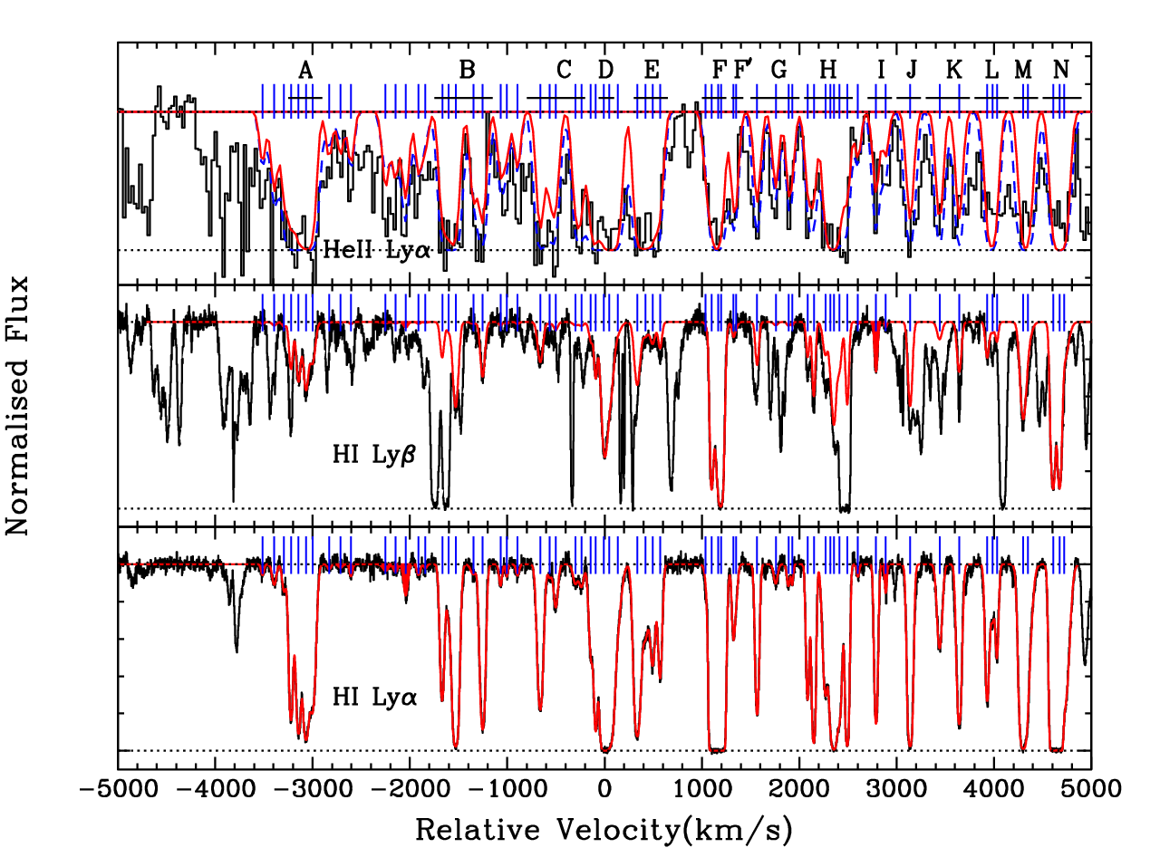


In this Section we concentrate on the column density ratio = (He ii)/(H i) over the redshift range 2.58 where the FUSE data show relatively good signal to noise ratio. This range roughly corresponds to a relative velocity range of 4000 km s-1 to 5000 km s-1 around the strong O vi absorber seen at = 2.6346 (see Fig. 1).
As a first step we fitted simultaneously the Lyman- to Lyman- profiles when possible, e.g. when the Lyman- and/or Lyman- lines are not blended with another intervening Lyman- line. Then we compare the He ii absorption profile with a model with the same components as the H i model, scaling the fitted H i column densities by the parameter . We consider two alternatives: In the first case we use the same Doppler parameter for H i and He ii (assuming turbulent broadening); in the second case we give the He ii -parameter the value expected from thermal broadening (i.e (He ii) = 0.5(H i)). The best fitted values of is obtained by minimization. While fitting the He ii profiles we use a Gaussian convolving function to correctly represent the FUSE spectral resolution. For Voigt-profile decomposition we have used the fitting code developed by Khare et al. (1997).
As the FUSE data are of much lower resolution and SNR than the UVES data, we cannot estimate for individual H i components. Instead, we have singled out 15 small regions named as A, B, C etc., in Fig. 1 and we derive the best value over each region. We wish to point out that the approach we have taken here is very different from previous studies. Indeed, Shull et al. (2004) used apparent optical depth in Lyman- only (AOD) method, whereas Kriss et al. (2001) and Zheng et al. (2004) used Gaussian decomposition and Fechner & Reimers (2007) scale the whole H i spectrum by = to fit the He ii data. In all these studies only H i Lyman- is used 22 2 limited amount of analysis of Lyman- have been done by Zheng et al. (2004).. This is the use of the H i optical depths in all available Lyman series lines that allows us to discriminate between thermal and turbulent broadening.

The best fitted Voigt profiles to the Lyman- and Lyman- absorption lines are shown in the bottom and middle panels of Fig. 1. The top panel shows the best fitted He ii Lyman- line with the two assumptions on the Doppler parameter discussed above. The curves as a function of for the different regions singled out in Fig. 1 are shown in Fig. 2. The solid and dashed lines in these plots represent the cases of thermal and turbulent broadening respectively. In most cases the curve shows a clear minimum thereby allowing us to discriminate between the turbulent and thermal cases, and to derive the best fitted value of . Errors are estimated from the range of values corresponding to = 1 around the minimum. There are regions, especially when the He ii Lyman- line is saturated, for which the curve flattens (e.g. regions E and G), we have only one-sided limit. In these cases we define the 2 lower limit of as the value corresponding to a equal to of the flat part of the curve plus four. The shapes of the curves are not symmetric which is a natural consequence of line saturation.
It is clear from the Figure that, apart from region I, the values are smaller in case of turbulent broadening and that minima are reached only in that case. In the case of thermal broadening, the curves seem to saturate to some asymptotic value probably because the observed He ii profiles are too broad to be reproduced by the model. Thus the exercise presented here shows that the width of He ii Lyman- lines are consistent with the -parameter derived from H i lines.
If the gas is optically thin and photo-ionized by a UV background dominated by QSOs, we would expect to be in the range 40400 depending on the exact spectral index and the IGM opacity. In the case of self-shielded optically thick gas, could be even higher (Fardal et al., 1998). Four regions (D, F, H and N) in Fig. 2 have . These regions are associated with large H i column densities as can be seen on Fig. 3 where log is plotted against log (H i) as measured in the different regions. This correlation was already noted in earlier works. Fechner & Reimers (2007) argued that this can be explained if the thermal broadening of lines are also important.
In the following, we will use additional information on metal lines observed in the UVES spectrum to discuss further the ionization state of the gas in these regions.
4 Regions with low values
In the previous Section, we have shown that the (He ii)/(H i) ratio can be explained over most of the observed spectrum by ionization of the gas by the UV background except in four regions: D (= 2.6346), F (= 2.6498), H (= 2.6624) and N (= 2.6910). The presence of O vi and C iv absorption in systems showing low values of may yield interesting clues about (i) the nature of the ionizing radiation, (ii) the effect of thermal/turbulent broadening and (iii) the possible mechanical feedback from winds.
Regions D and F are associated with C iv and strong O vi absorption lines. These are the only two C iv systems in the redshift range (see top panels in Fig. 4) and we discuss them in detail below.
For region H, the wavelength range where possible O vi1031 absorption is redshifted is strongly blended and only a possible weak line is present at the expected location of O vi1037 (see bottom-left hand-side panel in Fig. 4). As no other metal line is detected at this redshift we are unable to confirm if this feature is indeed due to O vi absorption.
For region N, while both O vi regions are strongly blended, the optical depth constraints are satisfied at two velocity positions (see Fig. 4). However, the possible O vi1031 feature is also consistent with being C iii absorption at 2.8972. Similarly, the possible O vi1037 line is blended with Lyman- at = 2.7306 and O vi1031 at = 2.7121. Hence, we cannot confirm the presence of O vi absorption in this region. Note that in region N (i.e. = 2.6910) is probably affected by transverse proximity effect from QSO J23495-4338 located at redshift 0.006, 15 arcmin away from the line of sight of interest (Worseck et al., 2007).


Note that we detect O vi absorption at = 2.7121, 2.7356 and 2.7456 as well. The He ii opacity is high at = 2.7121 and 2.7456 which makes difficult to estimate. If we scale the Voigt-profile fits to the H i absorption to reproduce the He ii profile, we find to be in the range 10100 and 100 for, respectively, the systems at = 2.7121 and 2.7456. The wavelength range in which the He ii absorption at = 2.7356 is expected to be redshifted has been removed by Zheng et al. (2004) because of the strong airglow lines so that we cannot estimate for this system. The system at = 2.7356 is a known Lyman-limit system. A Voigt-profile fit to the H i absorption gives log = 16.500.28.
4.1 System at = 2.6498
A velocity plot of high ionization metal lines and H i lines from this system is shown in the top-right panel of Fig. 4. Clearly the metal lines are off-centered with respect to the H i absorption. In addition, there is a velocity off-set of 2 to 10 km s-1 between the centroids of the O vi and C iv absorption profiles. Interestingly, all the shifts are in the same direction as would be expected in a flow ionized from the same side. The best fit of the profiles is obtained when we allow for C iv component redshifts to be independent of that of the O vi components (see Table 1).
Doppler parameters are larger for O vi compared to C iv which supports neither pure thermal nor pure turbulent broadening. The upper limits on the kinetic temperature of the gas measured from the -parameters of O vi components is 1.4, 8, 1.2 and 4 K respectively for components at , , and km s-1. Therefore within the allowed error in -parameters, the O vi profile allows for the existence of high temperature ( K) at least in part of the associated gas.
The top panel of Fig. 5 shows the apparent column densities of O vi (in blue) and C iv (in red) per unit velocity interval versus relative velocity. Since O vi 1037 is heavily blended we use only the O vi1031 line. For C iv, we have used the oscillator strength weighted mean of the column densities per unit velocity measured from both absorption lines of the doublet. For clarity, we have multiplied the C iv apparent column density profile by a factor of 10. Vertical dashed and dotted lines show the positions of peaks in the optical depth of C iv and O vi respectively. It is apparent that the O vi peaks are shifted compared to the C iv ones.

In the lower panel of Fig. 5 we plot the ratio of O vi to C iv apparent column densities per unit velocity against the relative velocity and find that the ratio varies between 10 and 20 through the C iv absorption profile. The fact that the O vi absorption profile is broader suggests the existence of gas outside the C iv profile with O vi to C iv column density ratio higher than 20.
The component at km s-1has virtually no detectable H i absorption associated. From the Lyman- line we derive an upper limit of log (H i) = 12.80 suggesting that metallicity is probably high in this component. Indeed, given the low value of the component, it is probable that the gas is photo-ionized in which case metallicity has to be close to solar. For the other three components that coincide with a strong H i absorption and it is impossible to quantify the amount of H i absorption associated with them individually such that useful metallicity limits can be established.
| (km s-1) | Ion | H i lines used | (km s-1) | log ( in cm-2) |
|---|---|---|---|---|
| 214.6 1.0 | H i | Ly- | 16.3 1.5 | 12.59 0.03 |
| 150.8 0.3 | H i | Ly-, Ly- | 23.6 0.3 | 14.63 0.01 |
| 76.2 0.0 | H i | Ly-, Ly- | 37.6 0.9 | 14.91 0.01 |
| 48.6 0.0 | H i | Ly-, Ly- | 23.1 0.7 | 14.68 0.02 |
| 20.2 0.0 | H i | Ly-, Ly- | 26.4 1.1 | 13.53 0.06 |
| 76.2 3.3 | O vi | 38.6 3.9 | 13.56 0.05 | |
| 58.8 1.0 | C iv | 14.5 1.5 | 12.30 0.03 | |
| 48.6 0.3 | O vi | 9.4 0.9 | 13.16 0.06 | |
| 24.1 0.6 | C iv | 5.9 1.0 | 12.06 0.04 | |
| 20.2 0.2 | O vi | 10.9 0.4 | 13.55 0.02 | |
| 1.9 0.4 | C iv | 4.8 0.7 | 12.16 0.03 | |
| 4.2 0.1 | O vi | 6.5 0.2 | 13.49 0.01 |
We have seen before (Fig. 2) that the curve corresponding to the fit of the He ii absorption shows a marked minimum for = 12 in the case of turbulent broadening (i.e = = 1) and no minimum for pure thermal broadening ( = 0.5). In Fig. 6 we show in the left hand-side row the simulated He ii profiles for 130 and = 0.5 (solid curve) and 12 and = 1.0 (dashed curve). Remember that for these fits we have used the minimum number of Voigt profile components without any constraint from the O vi profile. It is apparent that the red solid He ii profile (obtained assuming pure thermal broadening) is missing several pixels in the red wing of the region of interest around 0 km/s. This is because the value of the corresponding component (fixed by the H i profile) must be much larger to reach this position. If we now add the constraint that H i should be associated with the three O vi components, we can reproduce this profile better. Indeed, because of the extra component at km/s, pure thermal broadened He ii profile with higher ( 100) gives an equally good fit (right panel of Fig. 6).
It seems therefore that if we add a He ii component at the position of the redder O vi component, any value of between 15 and 100 is acceptable. Thus it seems that the possible presence of unresolved narrow H i components could be one of causes of low measurements. It is a fact however that the main H i components have large values, corresponding to temperatures in excess of 105 K. Therefore it is not impossible that part of the gas is at high temperature.
4.2 System at = 2.6346
| (km s-1) | Ion | H i lines used | (km s-1) | log ( in cm-2) |
|---|---|---|---|---|
| 140.6 0.0 | H i | Ly- | 27.8 0.6 | 13.41 0.01 |
| 91.6 0.0 | H i | Ly-,Ly-,Ly- | 22.5 0.3 | 13.80 0.01 |
| 16.4 0.2 | H i | Ly-,Ly-,Ly- | 38.2 0.9 | 14.27 0.03 |
| O vi | 20.3 8.3 | 12.76 0.28 | ||
| C iv | 11.5 2.4 | 12.55 0.12 | ||
| 0.6 0.7 | H i | Ly-,Ly-,Ly- | 28.3 2.2 | 14.14 0.06 |
| O vi | 18.9 0.5 | 14.05 0.02 | ||
| C iv | 8.1 0.6 | 12.83 0.06 | ||
| 36.2 0.7 | H i | Ly-,Ly-,Ly- | 25.7 10.4 | 13.24 0.37 |
| O vi | 9.6 0.8 | 13.37 0.04 | ||
| C iv | 7.5 1.0 | 12.19 0.04 | ||
| 48.5 0.0 | H i | Ly-,Ly-,Ly- | 46.6 1.5 | 14.32 0.01 |
| O vi | 25.2 1.6 | 13.61 0.03 | ||
| 101.4 0.0 | H i | Ly-,Ly- | 69.5 2.0 | 13.69 0.02 |
| O vi | 32.8 3.5 | 13.35 0.04 |
Absorption profiles from this system are shown on a velocity scale in Fig. 4. Unlike in the previous system the velocity range of metal lines falls well within the Lyman- profile. The O vi1037 line is blended with Lyman- at = 2.8781 and Lyman- at = 2.6765. Because of this contamination we use the well measured redshifts of C iv components to fit the O vi doublet. The contributions of the contaminating lines are self-consistently computed using other available transitions. In addition to the C iv counterparts, we need two components in the red part of the profile to fit the O vi doublet where there is no C iv absorption. H i Lyman-, Lyman-, and Lyman- lines have been fitted simultaneously imposing components at the redshifts of five O vi components. Two extra components are required in the blue ( km/s) to cover the total H i absorption. The details of the fit results are given in Table 2.
As in the previous system, for the components with both C iv and O vi the O vi -parameters are larger than the C iv ones and the column density ratio of O vi to C iv is as high as . The O vi -parameters correspond to upper limits on the kinetic temperature of , and K respectively for the components at , and km s-1. In the components where we find only O vi the ratio of O vi to C iv column densities can be higher than 20. These components have broad O vi lines with -parameters corresponding to upper limits of and K respectively for the components at and km s-1. The corresponding H i components also have high values allowing for high temperature ( K) in the gas associated with these two components. All this suggests a multiphase structure in this absorbing gas with the possible existence of a hot phase contributing to most of the O vi absorption. Indeed, the O vi profile is suggestively broad.


We fitted the H i and He ii profiles in the two extreme cases of pure turbulent and pure thermal broadening, considering both components from the fit of the H i profile only and from the fit of metal lines. Results are given in Fig 7 and Table 2. We notice from right panel of Fig 7 that even when we tie the H i components to O vi components the best fitted is obtained for the pure turbulent case with low . However, reality probably corresponds to an intermediate case with between 0.5 and 1. In the bottom panel of Fig. 8 we plot the minimum value obtained for different values of . Even though the best fitted value is obtained for = 1 the curve is flat and the 1 range is . As can be seen in the top panel of the figure, this can accommodate a wide range of . Therefore, in this system also high values are acceptable although H i and O vi absorption profiles are broad and highly suggestive of a gas with temperature higher than the typical photo-ionization temperature (i.e few K).


5 Models
Given the particularities of the systems singled out by the presence of O vi absorption, possible low values and high O vi/C iv ratios, we have constructed models to test the different mechanisms that could induce such properties. It is well known that photo-ionization by a power-law spectrum with appropriate slope can yield low values. This would require the presence of local sources of hard photons (Shull et al., 2004, see). Observations by Worseck et al. (2007) seem to show however that there is no QSO present in the vicinity of the two absorbers considered in the previous Section. While this observation does not rule out a QSO emission highly beamed perpendicular to the line of sight or a short lived QSO emission in the vicinity of the absorbers, we explore alternate explanations for low in the O vi absorbers. Therefore, in the following we present the results of models of a hot gas embedded in the meta-galactic UV background.
We use the photo-ionization code Cloudy (v07.02; Ferland et al. (1998)) to derive the ionization structure in a gas with fixed temperature (therefore not controlled by photo-ionization). This will make it possible to discuss at the same time both extreme situations (collisional ionization and photo-ionization) but also the intermediate situation of high-temperature gas with a contribution of photo-ionization. For comparison, we also show results from the model in which the temperature is the consequence of thermal equilibrium under photo-ionization. The calculations are made in the optically thin case. We use the Haardt and Madau (2005) background spectrum dominated by QSOs. We assume relative solar abundances and [C/H] = . In the top panel of Fig. 9, we plot the variation of the O vi to C iv ratio with hydrogen density. The solid black line is the result of model calculations where temperature is calculated by CLOUDY assuming photo-ionization equilibrium. Other lines are for temperatures in the range 51045105 K. It is to be remembered that when pure collisional excitation is considered the fraction of He ii is maximum when 4.5 4.9 and in the case of O vi it is 3 K (Gnat & Sternberg, 2007). At low temperature (say K) the ionization is dominated by photo-ionization. As expected the transition between photo-ionization dominated and collisional ionization dominated regimes happens at K.
The horizontal dotted lines show the range of observed O vi to C iv column density ratios (between 10 and 20) seen in the C iv components of the two systems discussed above. This range is well reproduced by models with T K for a typical density of 10-4 cm-3. However the higher O vi to C iv ratio inferred in the velocity range (or Voigt profile components) where only O vi is detected needs either low density (and low temperature) photo-ionized gas or high density (i.e cm-3) hot gas (T K) where collisions begin to play a role. Interestingly such high temperatures are not ruled out by the -parameters of O vi components (see discussions in the previous Section).


In the bottom panel of Fig. 9 we plot as predicted by the models versus the hydrogen density. It is apparent that low values (i.e ) are only possible for K. Available data on H i and He ii profiles allow for the existence of such hot gas that would also produce the component with high O vi to C iv column density ratio (i.e (O vi)/(C iv)20). It is apparent from Fig. 4 that the absorption profiles indicate higher Doppler parameters going from C iv to O vi to H i. This has already been noted for C iv and O vi by Fox et al. (2007) and interpreted as the existence of a hot phase. We note that the values measured for the strongest H i components in the two systems (38.6 km/s at = 2.6498 and 46.6 and 69.5 km s-1 at = 2.6346, see Tables 1 and 2) are consistent with a temperature, K and it is apparent from the absorption profiles that larger values could be accommodated.
If the low values were to be confirmed, we would favor a scenario where the absorbing gas is a multiphase medium in which photo-ionized gas components coexist with a wide range of density and temperature. While most of the metal absorption traced by C iv comes from relatively cold (i.e T K) gas part of O vi and predominant contributions of H i and He ii could be due to a hot phase ( K). There is evidence for the existence of multiphase media in the low-z O vi absorbers (Tripp et al., 2008) and O vi absorption associated with high- DLAs (Fox et al., 2007).
6 Conclusions
We have reanalyzed the line of sight towards the high redshift ( = 2.885) bright quasar QSO HE 23474342 and measured the parameter = (He ii)/(H i) in the Lyman- forest using Voigt-profile fitting of the H i transitions in the Lyman series. As in previous studies, we find that in most of the Lyman- forest except in four regions where it is much smaller ().
We detect O vi absorption associated with two of these regions (at = 2.6346 and 2.6498). The corresponding wavelength ranges for the two other regions are too blended to reach any firm conclusion on the presence of associated O vi absorption. We observe that the = 2.6346 system is a usual system with the metals located at the center of the H i profile whereas the = 2.6498 system has the metals displaced in the red wing of the H i absorption but moreover, with the C iv profile systematically shifted compared to O vi. Doppler parameters of the well-defined C iv components rule out the fact that the associated gas is hot and favor the idea that this gas is photo-ionized. We show that if we constrain the fit of the H i and/or He ii absorption profiles with the presence of metal components, we can accommodate values in the range 15–100 in these systems assuming broadening is intermediate between pure thermal and pure collisional.
We construct constant density photo-ionized models and show that while simple photo-ionization models reproduce the observed (O vi)/(C iv) ratio for a range of density, they fail to produce low values. On the contrary, models with high temperature (i.e T K) can produce low values of . The Doppler parameters of the strongest H i components are consistent with such a temperature. In addition, the higher values observed for O vi compared to C iv and the existence of O vi alone components suggest a multiphase nature of the absorbing region. Therefore, if low values were to be confirmed, we would favor a multi-phase model in which most of the gas in the regions of low is at high temperature (105 K) but the metals and in particular C iv are located in lower temperature photo-ionized and probably transient regions. As the high temperature gas can not be produced by photo-ionization, we expect the O vi systems with low to be associated with galaxies. Therefore, deep search for Lyman break galaxies at these redshifts may be interesting to perform in these fields.
Acknowledgment
We wish to thank Dr. Zheng for providing the FUSE data and the referee Dr. Williger for useful comments. SM thanks CSIR for providing support for this work. RS thanks University Paris 6 and IAP for an invitation as Professeur Associé.
References
- Aguirre et al. (2008) Aguirre, A., Dow-Hygelund, C., Schaye, J., & Theuns, T., 2008, ApJ, 689, 851
- Aracil et al. (2004) Aracil, B., Petitjean, P., Pichon, C., & Bergeron, J., 2004, A&A, 419, 811
- Ballester et al. (2000) Ballester, P., Modigliani, A., Boitquin, O., Cristiani, S., Hanuschik, R., Kauffer, A., & Wolf, S., 2000, The Messenger, 101, 31
- Bergeron et al. (2002) Bergeron, J., Aracil, B., Petitjean, P., & Pichon, C., 2002, A&A, 396, L11
- Bergeron et al. (2004) Bergeron, J., Petitjean, P., Aracil, B., et al., 2004, The Messenger, 118, 40
- Bouché et al. (2007) Bouché, N., Lehnert, M. D., Aguirre, A., Péroux, C., & Bergeron, J., 2007, MNRAS, 378, 525
- Bouché et al. (2006) Bouché, N., Lehnert, M. D., & Péroux, C., 2006, MNRAS, 367, L16
- Chand et al. (2004) Chand, H., Srianand, R., Petitjean, P., & Aracil, B., 2004, A&A, 417, 853
- Davé et al. (2001) Davé, R., Cen, R., Ostriker, J. P., et al., 2001, ApJ, 552, 473
- Dekker et al. (2000) Dekker, H., D’Odorico, S., Kaufer, A., Delabre, B., & Kotzlowski, H., 2000, in Proc. SPIE Vol. 4008, p. 534-545, Optical and IR Telescope Instrumentation and Detectors, Masanori Iye; Alan F. Moorwood; Eds., pp. 534–545
- Edlén (1966) Edlén, B., 1966, Metrologia, 2, 71
- Ellison et al. (2000) Ellison, S. L., Songaila, A., Schaye, J., & Pettini, M., 2000, AJ, 120, 1175
- Fang & Bryan (2001) Fang, T. & Bryan, G. L., 2001, ApJ, 561, L31
- Fardal et al. (1998) Fardal, M. A., Giroux, M. L., & Shull, J. M., 1998, AJ, 115, 2206
- Fechner & Reimers (2007) Fechner, C. & Reimers, D., 2007, A&A, 461, 847
- Ferland et al. (1998) Ferland, G. J., Korista, K. T., Verner, D. A., Ferguson, J. W., Kingdon, J. B., & Verner, E. M., 1998, PASP, 110, 761
- Fox et al. (2007) Fox, A. J., Petitjean, P., Ledoux, C., & Srianand, R., 2007, A&A, 465, 171
- Gnat & Sternberg (2007) Gnat, O. & Sternberg, A., 2007, ApJS, 168, 213
- Haardt & Madau (1996) Haardt, F. & Madau, P., 1996, ApJ, 461, 20
- Kang et al. (2005) Kang, H., Ryu, D., Cen, R., & Song, D., 2005, ApJ, 620, 21
- Khare et al. (1997) Khare, P., Srianand, R., York, D. G., Green, R., Welty, D., Huang, K., & Bechtold, J., 1997, MNRAS, 285, 167
- Kriss et al. (2001) Kriss, G. A., Shull, J. M., Oegerle, W., et al., 2001, Science, 293, 1112
- Oppenheimer & Davé (2009) Oppenheimer, B. D. & Davé, R., 2009, MNRAS, 395, 1875
- Pieri et al. (2010) Pieri, M. M., Frank, S., Mathur, S., Weinberg, D. H., York, D. G., & Oppenheimer, B. D., 2010, ApJ, 716, 1084
- Reimers et al. (1997) Reimers, D., Kohler, S., Wisotzki, L., Groote, D., Rodriguez-Pascual, P., & Wamsteker, W., 1997, A&A, 327, 890
- Scannapieco et al. (2006) Scannapieco, E., Pichon, C., Aracil, B., Petitjean, P., Thacker, R. J., Pogosyan, D., Bergeron, J., & Couchman, H. M. P., 2006, MNRAS, 365, 615
- Schaye et al. (2003) Schaye, J., Aguirre, A., Kim, T.-S., Theuns, T., Rauch, M., & Sargent, W. L. W., 2003, ApJ, 596, 768
- Shull et al. (2004) Shull, J. M., Tumlinson, J., Giroux, M. L., Kriss, G. A., & Reimers, D., 2004, ApJ, 600, 570
- Shull et al. (2010) Shull, M., France, K., Danforth, C., Smith, B., & Tumlinson, J., 2010, arXiv:1008.2957
- Simcoe et al. (2004) Simcoe, R. A., Sargent, W. L. W., & Rauch, M., 2004, ApJ, 606, 92
- Smette et al. (2002) Smette, A., Heap, S. R., Williger, G. M., Tripp, T. M., Jenkins, E. B., & Songaila, A., 2002, ApJ, 564, 542
- Songaila & Cowie (1996) Songaila, A. & Cowie, L. L., 1996, AJ, 112, 335
- Srianand & Petitjean (2000) Srianand, R. & Petitjean, P., 2000, A&A, 357, 414
- Stumpff (1980) Stumpff, P., 1980, A&AS, 41, 1
- Tripp et al. (2008) Tripp, T. M., Sembach, K. R., Bowen, D. V., Savage, B. D., Jenkins, E. B., Lehner, N., & Richter, P., 2008, ApJS, 177, 39
- Worseck et al. (2007) Worseck, G., Fechner, C., Wisotzki, L., & Dall’Aglio, A., 2007, A&A, 473, 805
- Zheng et al. (2004) Zheng, W., Kriss, G. A., Deharveng, J., et al., 2004, ApJ, 605, 631