Jet quenching in hot strongly coupled gauge theories revisited: 3-point correlators with gauge-gravity duality
Abstract
Previous studies of high-energy jet stopping in strongly-coupled plasmas have lacked a clear gauge-theory specification of the initial state. We show how to set up a well-defined gauge theory problem to study jet stopping in pure super Yang Mills theory (somewhat analogous to Hofman and Maldacena’s studies at zero temperature) and solve it by using gauge-gravity duality for real-time, finite-temperature 3-point correlators. Previous studies have found that the stopping distance scales with energy as (with disagreement on the gauge coupling dependence). We do find that none of the jet survives beyond this scale, but we find that almost all of our jet stops at a parametrically smaller scale proportional to , where is the size of the space-time region where the jet is initially created.
I Introduction and Results
How far does a localized, high-energy excitation travel in a quark-gluon plasma before slowing down, stopping, and thermalizing? This question is of phenomenological interest for heavy ion collisions, and it has long been a problem of theoretical interest to calculate the result in various idealized situations. In a weakly-coupled gauge theory with massless partons, the stopping distance scales with energy as , up to powers of logarithms, where is the initial energy of a high-energy parton.11 1 A specific calculation for QCD of the stopping distance at weak coupling in the high-energy limit may be found in Ref. [1]. However, the scaling of this result was implicit in the early pioneering work of Refs. [2, 3] on bremsstrahlung and energy loss rates in QCD plasmas. At the other extreme, investigations [4, 5, 6] of strongly-coupled, large-, supersymmetric versions of QCD, using gauge-gravity duality [7, 8, 9, 10], have indicated that the maximum stopping distance scales like . In this paper, we revisit this gauge-gravity duality result. In particular, previous calculations have always specified the high-energy initial state using the gravity description (and in some cases relegated other matters of interpretation to the gravity description): there has not been a complete specification of the problem, from beginning to end, solely in terms of 4-dimensional gauge theory. We will investigate what happens if a localized, high-energy excitation is created in the gauge theory, and the response later measured in the gauge theory. For our method of creating the initial excitation, we find that there is an additional scale characterizing the response: almost all of the excitation’s conserved charge is deposited at a distance that scales with energy as rather than and is sensitive to the initial spatial size of the excitation. Nonetheless, we will still see emerge as the furthest distance that any non-negligible fraction of the charge propagates before stopping and thermalizing.
To be more concrete, we need to explain more precisely what we calculate.
I.1 The problem
The specific theory we study is pure super Yang Mills theory in the large and large limit. Readers needing a general introduction to the use of gauge-gravity duality to study finite-temperature physics in this and similar strongly-coupled theories should refer to Ref. [12].
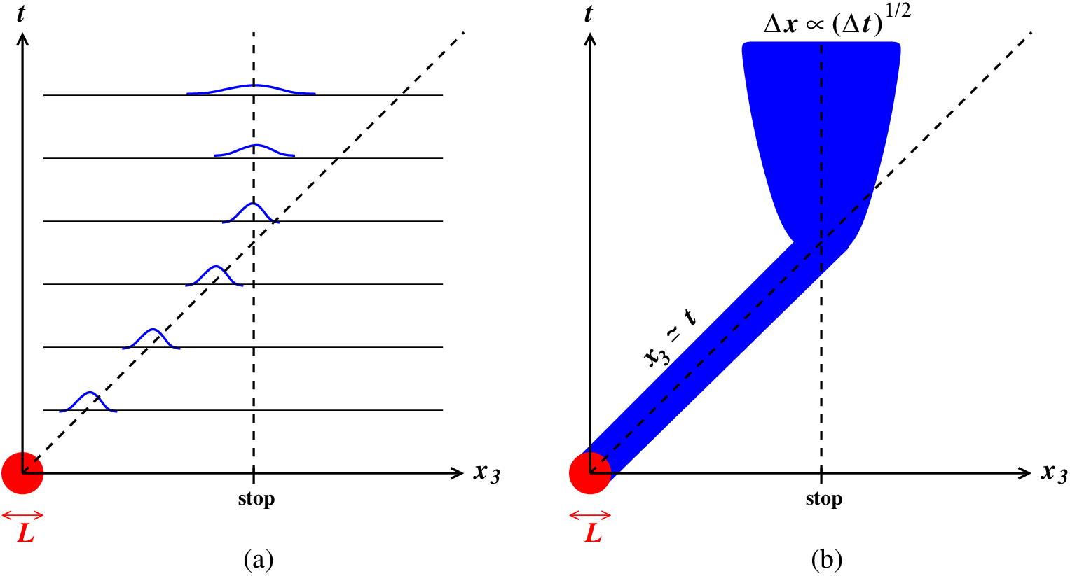
We will follow the general philosophy of Chesler et al. [6, 11] that the way to study stopping distances is to locally create a high-energy excitation and then measure the subsequent evolution of conserved charge densities such as energy or momentum density. A cartoon of this evolution is shown in fig. 1. In contrast to previous studies at finite temperature , we will give an explicit gauge theory prescription for creating the initial excitation. We excite the gauge theory plasma by turning on external sources, localized in space-time, that produce a high-energy state with nearly-definite energy and momentum. One could in principle use most any type of source that has a simple translation to the gravity dual theory under the AdS/CFT correspondence, but in this paper we will focus on an example where the sources couple to the global R-charge currents of the gauge theory. It will also simplify the analysis to use a source that is translation invariant in the two spatial dimensions transverse to the motion of the excitation, but localized in time and the third space direction. Specifically, we modify the 4-dimensional field theory Lagrangian by
| (1) |
where are the SU(4) R-charge currents of the theory and is a classical external source. We choose the external source to have the form of (i) a high-energy plane wave times (ii) a smooth, slowly varying, real-valued envelope function localizing the source to a space-time region of size . Specifically,
| (2) |
where
| (3) |
is a very large light-like 4-momentum with frequency ; is an arbitrarily small source amplitude; is a transverse linear polarization, such as
| (4) |
and are Pauli matrices for any SU(2) subgroup of the SU(4) R-symmetry, with
| (5) |
(The motivation for the factor will be discussed below). A simple example of an appropriate envelope function would be
| (6) |
should be chosen large compared to , so that the momentum components in the source are all close to (3), but small compared to the large stopping distance that we wish to study. To avoid the mental clutter of an over-abundance of scales, it is convenient (but not necessary) to consider to be of order in what follows.
The source (2) creates an excitation that carries energy, momentum, and R charge. We could subsequently track the densities of any of these conserved charges to study the evolution of the excitation. In this paper, we have chosen to study the evolution of the R charge density, specifically the large-time behavior ( both and ) of
| (7) |
if the system starts in thermal equilibrium at . Here, the superscript “” indicates the R charge current associated with in the SU(2) subgroup referenced by (5), and the subscript “” indicates that the expectation is taken with the source term (1) present in the Lagrangian. Because of the in (2), the situation is analogous to the interaction of a quark-gluon plasma with an external, high-energy boson in a wavepacket of size (and with a decay time of order ), as depicted in fig. 2.22 2 One could imagine strengthening this analogy by gauging an SU(2) subgroup of the super Yang Mills R symmetry with a very weak coupling constant . The full SU(4) R symmetry is anomalous and so cannot be consistently gauged unless one adds yet other fields to the model to cancel the anomaly. But an SU(2) subgroup is not anomalous and could be gauged, provided one defines the currents of that subgroup appropriately. The currents that the gauge bosons would have to couple to would be slightly different than the usual currents defined in the AdS/CFT correspondence with holographic regularization because the latter treat all the R currents on an equal footing. This difference in currents reflects the difference between the covariant and consistent anomalies [13]. None of these distinctions actually matter in the current problem with source (2), but we will simply avoid gauging any of the R currents so that we do not need to ponder these issues. The boson will leave behind an excitation that carries electric charge and the third component of isospin . Subsequently measuring the latter is analogous to (7).

I.2 The result
We will take the source amplitude to be arbitrarily small so that we can treat the source term (1) as a small perturbation in our later analysis. A small-amplitude source will most of the time have no effect at all on the system, producing no excitation and no R charge. We can normalize away this case simply by dividing the average charge density distribution by the average total charge produced by the source,
| (8) |
In the case of a transverse-translational invariant source, such as will be studied in this paper, it is more appropriate to consider the charge per unit transverse area .
The simplest way to express our final result is to give a charge-deposition function which represents how much thermalized charge the high energy excitation leaves behind at each space-time point . More specifically, is the source term for the diffusion equation for the subsequent evolution of that charge, so that the late-time charge density is given by33 3 The idea of defining and investigating has been taken from Chesler, Jensen, and Karch [11]. However, in that paper, they applied it only to scales large compared to the stopping distance of the high-energy excitations. Here, we resolve all scales where hydrodynamics is applicable.
| (9) |
where the here indicates that we are only resolving structure on distance and times scales large compared to the thermal wavelength . For a strongly-coupled plasma, that is the hydrodynamic limit—the limit where the diffusion equation is applicable. The value of the R-charge diffusion constant is [14]
| (10) |
Our result is that, if one contents oneself with only resolving details on distance scales large compared to both the source size and the thermal wavelength , then
| (11) |
where is the step function; ; and is a source-dependent function that suppresses , causing suppression of above. In the case of the Gaussian source (6),
| (12) |
The subscript on indicates that is only an approximate delta function, with a width of order . Approximating it as a true delta function is good enough if we are only interested in the hydrodynamic response on scales large compared to . In (11), the ’s are numerical constants, given by
| (13) |
We shall see later that and are determined by the first quasi-normal mode in the gravity description.
A qualitative summary of the the dependence of is shown in fig. 3. The deposition of charge furthest from the origin that is not exponentially suppressed is at
| (14) |
which scales with energy as like the various results of Refs. [4, 5, 6]. However, at least on average, only a tiny fraction of the total charge is deposited at this distance if we keep the source size small compared to itself. Most of the charge is deposited at the much smaller distance scale
| (15) |

There is an important difference between (14) and the subset [4, 6] of earlier results which have studied jet stopping by studying the dynamics of classical strings on the gravity side. Ref. [6] (see also [11]) added massless fundamental-charge matter to supersymmetric Yang Mills and argued that one could study the stopping of excitations carrying the analog of baryon number by studying the stopping of moving classical strings in the gravity dual. Ref. [4] studied the pure Yang-Mills theory and modeled gluon jets by the evolution of folded pieces of string in the gravity dual. In both references, the stopping distance was found to be of order
| (16) |
which is parametrically smaller than our corresponding scale (14) by a factor of in the strong-coupling limit . Formally, the origin of the factor of in the calculations based on classical strings is the fact that the string tension, and therefore the energy of the state represented by the string, is proportional to , so that . In our calculation, in contrast, we will not consider classical strings at all. We will just use the most basic, original elements of the AdS/CFT dictionary for relating gauge theory operators to classical boundary sources in the gravitational dual.
Our maximal scale (14) does agree (including the absence of ) with the scale previously found by Hatta, Iancu, and Mueller [5], who specifically studied R charge excitations like we do. Gauge-gravity duality relates the SU(4) R currents to classical 5-dimensional SU(4) gauge fields on the gravity side. They studied how a wave solution of the gravity-theory fields would fall into the black brane horizon, and then they used rough, qualitative arguments to relate this behavior back to what happens in the 4-dimensional gauge theory. In this paper, we precisely relate the field theory problem we have outlined to a calculation in the gravity dual. Along the way of solving the gravity dual problem, we will eventually encounter the same sort of problem studied by Hatta, Iancu, and Mueller. However, we will find another scale to the problem, which was missed in their qualitative interpretation, and which corresponds to the scale (15) at which almost all of the charge is deposited. In fact, we will see that the appearance of this scale from the gravity calculation is intimately related to the conservation of R charge in the 4-dimensional gauge theory problem after the source turns off ().
Before moving on, we record the generalization of our result (11) to the case of a generic source envelope, which is that
| (17) |
where is the step function and is the two-dimensional Fourier transform
| (18) |
Provided the envelope function is smooth on the scale and falls sufficiently rapidly for , the qualitative conclusions are the same as for the Gaussian envelope.
I.3 Jets in strong coupling
We loosely use the term “jet” to refer to a spatially localized, high energy excitation that initially moves at nearly the speed of light through the plasma. There is a potential for confusion because sometimes people loosely summarize the (zero temperature) results of Hofman and Maldacena [15] as indicating that there are no jets in strongly-coupled super Yang Mills. Hofman and Maldacena considered the case of an isotropic source localized in all four space-time dimensions, with 4-momentum narrowly peaked around . In weak coupling, this source would predominantly produce two back-to-back partons, flying in opposite directions, and so produce a non-trivial angular distribution in the late-time energy-energy correlation function far away from the source. In the strong coupling limit, they found the opposite: there was no such angular correlation. Their source did not create a jet-like structure.
However, at zero temperature, one may change the appearance of something simply by boosting to a different reference frame. An expanding spherical shell of energy in the original frame looks like a single, slowly spreading, localized jet if one boosts by a very large amount in the direction. Effectively, this is what our source (2) does when we choose in (3). The envelope function causes a narrow spread in momentum around , and we will see later that it is the time-like subset () of these momenta that produce our result (see also [5]). So the physics of the creation of our initial “jet” state is essentially an extremely boosted version of the zero-temperature problem studied by Hofman and Maldacena.
Hofman and Maldacena related the measurement of one-point correlations of energy density to the calculation of three-point correlations , where was the operator that created their initial state. In order to measure charge densities such as (7) in this paper, we will similarly investigate three-point correlators (in our case at finite temperature) between (i) the measured charge density and (ii) operators associated with the creation of the source. However, for reasons of calculational simplicity that we will explain later, we have set up the problem in a slightly different way than Hofman and Maldacena did and so evaluate a slightly different type of 3-point correlator ordering. Specifically, we cast the problem in terms of retarded 3-point correlators.
I.4 What follows
In the next section, we set up the basic integrals that we will have to evaluate to obtain the charge density in terms of bulk-to-boundary propagators in AdS5-Schwarzschild space. Then we warm up to the task of evaluating these integrals in section III by applying our method to the simpler case of zero temperature. In particular, we will make comparison with Hatta, Iancu, and Mueller [5] in section III.5. We move on to the finite-temperature case in section IV, where we derive our final result (11). Finally, we conclude with some suggestions for future work in section V.
II General Set-up
II.1 Notational Preliminaries
We will use the form of the AdS5-Schwarzschild metric given by
| (19) |
where
| (20) |
is the radius of the AdS space-time (which results will not depend upon), corresponds to the 4-dimensional boundary, and corresponds to the horizon. For space-time indices, we will use capital roman letters (, , …) for indices in 5-dimensional space-time and Greek letters (, , …) for four-dimensional space-time. When we write a lower Greek index on a 4-momentum or polarization , we will always mean that the index is lowered with the 4-dimensional metric and not the 5-dimensional metric ; so
| (21) |
where .
Our conventions for light cone coordinates will be
| (22) |
and similarly
| (23) |
and so . When integrating over 4-momenta , we will use the short-hand notation
| (24) |
Where there is no opportunity for confusion, we will abbreviate as and sometimes even as .
II.2 Field Theory: 3-point functions
To relate the response of 1-point functions such as energy density or R charge density to equilibrium -point correlation functions, for small source amplitudes , one follows the same steps as in derivations of the fluctuation-dissipation theorem or Kubo formulas. Since it’s relatively simple, we’ll take a moment to review it here. Write the Hamiltonian as , where are the small-amplitude source terms and is everything else in the full Hamiltonian of the theory. If the system initially starts in equilibrium, before the sources turn on, then the later evolution of an observable is given by
| (25) |
where
| (26) |
is the evolution operator under , and is time ordering. Working in the interaction picture and expanding in powers of the small , one finds
| (27) |
where the various are the equilibrium -point retarded correlation functions, given in this case by44 4 Readers familiar with the (r,a) formalism may know these retarded Green functions as , , etc. See, for example, the review of notation in Ref. [16].
| (28) | ||||
| (29) |
etc. In our problem, the first non-vanishing term is the one involving the 3-point correlator because the operator has non-zero R-charge, causing the 2-point correlator to vanish. However, the conclusion is more general than our specific example involving R charge currents. To create a high-energy excitation, the source should have large momentum . To measure later hydrodynamic behavior after the jet stops in the medium, one wants to examine relatively low-wavenumber components of the late-time diffusing density . Because of this momentum mismatch between source and observable, the equilibrium two-point function will vanish by momentum conservation. It is only when we get to the three-point function that we first find a non-vanishing result.55 5 Hydrodynamic quantities like viscosity and charge diffusion constants can be studied using two-point correlators [14, 12, 17] because one may measure them by studying the low-wavenumber response of the system to a low-wavenumber source. The reason one has to go to 3-point functions here (and in Hofman and Maldacena [15]) is that we are specifically interested in a high-momentum source in order to study “jets.”
In our problem, (27) manifests in detail as
| (30) |
in the limit of arbitrarily small source amplitude .
Now comes a crucial argument that we will use repeatedly. In studying the response (30) to determine how far the jet travels, we will not care about the detailed structure on small distance and time scales such as or even . It would be perfectly adequate to look at a smeared response such as
| (31) |
where the smearing distance is chosen large compared to microscopic scales such as and but small compared to scales we’re interested in resolving, such as the stopping distances (14) and (15). In momentum space, the smearing (31) retains only small wavenumbers , by which we mean whose components are all . If we make an approximation to (30) that changes the integrand for large but not for small (where is conjugate to the point where we measure the charge density), then the smeared response (31) containing all the information we are interested in will not change. In the rest of this paper, we will not again explicitly reference the smeared response (31), but we will feel free to make approximations that are only valid when the components of have magnitudes small compared to and . Note that this only applies to the conjugate to the measurement point ; no such approximation would be acceptable for the source momenta and in (30), which are both large.
In particular, using the explicit source (2) in (30) gives
| (32) |
where we have ignored terms involving and because these contribute only to to very large momenta .
Before moving on to the gravity side of the calculation of retarded correlators, it will be useful to review the fact that retarded real-time correlators are related to time-ordered imaginary-time correlators by analytic continuation in frequency. For two-point correlators, we are used to seeing this in the form66 6 The imaginary-time -point Green function is defined here as times the imaginary-time time-ordered correlator of fields. So, for instance, for a free massless scalar.
| (33) |
where is the analytic continuation of the imaginary-time Green function to real-time frequencies;77 7 () indicates that one continues from positive (negative) imaginary frequencies. the upper and lower signs are for the retarded (R) and advanced (A) Green function respectively; and we have suppressed showing the spatial momentum . To understand the generalization to -point functions, it is useful to write the 2-point function in terms of two momenta, trivially related by momentum conservation:
| (34) |
Since , the prescription (33) is in this language
| (35) |
That is, the frequency associated with the response has a prescription and that associated with the source has the opposite. This generalizes to the higher-point functions, so that [18]88 8 One may check that the prescriptions (36) enforce vanishing of the retarded correlator unless is the largest of the three times, just as in the equivalent but more explicit formula (29). (i) Fourier transform (36) back to , , and , (ii) use frequency conservation for the integration to rewrite as , and (iii) close the and/or integration contours in the lower half plane if and/or [realizing that the prescription (36) makes analytic in the lower half planes of and/or (corresponding to the upper-half plane of )].
| (36) |
II.3 Gravity Dual: 3-point functions
II.3.1 Basics
The AdS/CFT correspondence translates the problem of computing the 3-point Green function of R charge currents in strongly-coupled gauge theory to the problem of computing 3-point boundary correlators of classical gauge fields living in AdS5-Schwarzschild space. If we were interested in imaginary-time correlators, the boundary correlator would be given by the Witten diagram of fig. 4a, with the circle representing the boundary of imaginary-time AdS5-Schwarzschild space.

To start with a simpler example, if we were studying a 3-point boundary correlator of 5-dimensional scalar fields in the gravity theory with 3-point vertex , then the Witten diagram would give
| (37) |
where the are 4-momenta in the boundary theory, is the coordinate for the 5th dimension, and is the bulk-to-boundary propagator which solves the 5-dimensional imaginary-time classical equation of motion for the scalar field, appropriately normalized on the boundary. is the usual boundary regulator. In our calculation, there will turn out to be no divergences as , and so we will set for simplicity.
Imaginary-time AdS5-Schwarzschild spacetime is smooth, and we can integrate over the entire space-time without worrying about horizons or singularities. In real time, one in principle has to worry about such issues, but for the retarded 3-point propagator one can find the correct prescription simply by the analytic continuation (36) of the imaginary-time result:
| (38) |
where and solve the linearized 5-dimensional real-time equations of motion with retarded or advanced boundary conditions respectively. The result (38) was found in Ref. [20], where more discussion of both retarded and other 3-point correlators may be found. (See also the related discussion in Ref. [21].)
As a matter of convention, note that our 4-momenta , and are momenta in the gauge theory, and therefore they are the momenta conjugate to the boundary points in the bulk-to-boundary propagators. (The momenta conjugate to the 4-position of the bulk point are correspondingly , , and .) As a result, our convention is that a retarded bulk-to-boundary propagator refers to the case where information flows from the bulk to the boundary, and so corresponds to a solution where waves flow out of the horizon. Similarly, our advanced bulk-to-boundary propagator is the solution where waves flow into the horizon.99 9 Let us relate this to the notation of Son and Starinets [12]. Let be the 4-momentum conjugate to the boundary position and the 4-momentum conjugate to the bulk position. Then, in the scalar case, our corresponds to their . Note that . In position space, our retarded bulk-to-boundary propagator from a bulk point to a boundary point is . The last is the same as the advanced boundary-to-bulk propagator defined by (40). If one wished to describe a bulk wave falling from the boundary into the horizon, it would be given by or equivalently . The two are related by
| (39) |
Readers who find it awkward or confusing to think in terms of bulk-to-boundary flow rather than boundary-to-bulk flow may, if desired, rewrite our equations in terms of boundary-to-bulk propagators defined by
| (40) |
where is the 4-momentum conjugate to the bulk position.
The real-time Witten diagram associated with (38) corresponds to Figure 4b, and the bulk vertex lives exclusively in the right-hand quadrant of the Penrose diagram. This can be understood from the causality properties of the retarded and advanced bulk-to-boundary propagators in the analytic continuation (38) of the imaginary-time result (37). only has support when the bulk point is in the causal future of the boundary point, and only when the bulk point is in the causal past of the boundary point. Taking the boundary points to all be on the right-hand boundary, the combination of these causality constraints requires the bulk vertex to be in the right-hand quadrant. This argument is similar to the discussion by Caron-Huot and Saremi [22] of the “causal diamond” in their analysis of long-time hydrodynamic tails from one-loop gravity corrections to the 2-point retarded correlator.
It is the simple form (38) of the retarded correlator that led us to choose to set up the problem of studying jet evolution in terms of retarded correlators, rather than the type of correlators considered by Hofman and Maldacena, which would be more complicated to analyze at finite temperature.1010 10 Such correlators can be related to the retarded correlator. Since the source is localized, and we are only interested in measurements at times after the source turns off, we can rewrite the correlator in Schwinger-Keldysh (closed time path) notation as . Each subscript in designates whether the corresponding operator appears on (1) the first leg of the Schwinger-Keldysh integration contour ( to ) or (2) the second leg ( to ), and operators are ordered accordingly. Specifically, , where represents ordinary time ordering. (Since is our largest time, here, where is the average of using 1 and 2.) 3-point Schwinger-Keldysh propagators can all be (non-locally) related to retarded Green functions , , and (the distinction being which of the three operators is the latest time when defining “retarded”) and their complex conjugates. Explicit formulas (and more explanation of the notation) are given in Ref. [16]. Alternatively, see Ref. [20] for a discussion of different 3-point correlators directly in terms of integrating over both right and left quadrants in the gravity theory. (Beware that Ref. [20], following Ref. [23], uses a different convention for the Schwinger-Keldysh contour than Ref. [16]. This introduces factors of into the definition of , where .)
II.3.2 The vector-vector-vector vertex
The generalization of (38) from scalar interaction to vector interaction is that we need to use the vector-vector-vector vertex in the super-gravity (SUGRA) theory:
| (41) |
where the advanced and retarded bulk-to-boundary propagators have one 4-dimensional vector index () associated with the boundary point and one 5-dimensional vector index () associated with the bulk point and are normalized on the boundary so that
| (42) |
The vertex function is extracted from the cubic terms in the SUGRA interaction [8, 24]
| (43) |
where we work in real time, have only shown explicitly the cubic term in the Chern-Simons interaction, and
| (44) |
The term produces a 3-point vertex with R charge structure , whereas the Chern-Simons term (which reproduces the R charge current anomaly) yields . Here and are defined in terms of SU(4) Hermitian generators by , normalized by .
Recall that the currents in our source (2) and measurement (7) were chosen to lie in an SU(2) subgroup of SU(4). Since vanishes for SU(2), the Chern-Simons term will not contribute in our application.1111 11 An independent reason that the Chern-Simons term does not contribute in our problem is our choice of linear polarization for our source: the two ’s which attach to the source points on the boundary will give factors of and contracted with the , giving zero. So the only relevant contribution to the vertex comes from the cubic interaction
| (45) |
The factors of the AdS radius all cancel [the explicit above with the factors in from (19)]. If desired, one could simply set in the rest of the paper.
To get the vertex function in (41), substitute the three bulk-to-boundary propagators for the three ’s in (45) in all possible permutations. Since the problem studied in this paper is invariant under translation in the transverse directions, we will restrict attention to 5-dimensional gauge choices that respect this invariance. In particular, the bulk-to-boundary propagators will preserve transversality of polarization,
| (46) |
and transverse derivatives will vanish,
| (47) |
Here it is convenient to define a 5-dimensional in terms of 4-dimensional by
| (48) |
Putting everything together, the piece of (41) that contributes in our problem is then
| (49) |
where is the transverse piece of the bulk-to-boundary propagator. (Other than as an attempt to save space in equations, there is no significance to whether we write the R/A for retarded/advanced as subscripts or superscripts.) Switching to four-dimensional momentum space, and using the notation ,
| (50) |
II.3.3 Summary in gauge
The last formula (50) is simplest in gauge, where the last term vanishes. We will specialize to gauge in the remainder of the paper. Define by
| (51) |
Putting everything together and using , we then have
| (52a) | |||
| with | |||
| (52b) | |||
in gauge.
As it currently stands, (52) is challenging to evaluate. Our crucial approximation in what follows will be to replace in (52b) by its small- approximation valid for . As discussed earlier in section II.2, such approximations are adequate for the long-distance physics that we wish to study. As a simple example, for a massless bulk scalar field, the bulk-to-boundary propagator in the small- limit is [25, 12]1212 12 To have an expression valid all the way to the horizon, it is important not to expand in powers of the exponent as . For any fixed , the corrections to this truncation are not small when is close enough to the horizon that .
| (53) |
where . The approximation (53) has the nice property that it factorizes for :
| (54) |
If this were the propagator to use for in (52b), then the and integrals would factorize in (52a), greatly simplifying the calculation by allowing us to evaluate them independently. We will see in section IV that the issue of factorization is a little more complicated for the vector bulk-to-boundary propagator at finite temperature, but we will be able to use a variant of this trick to factorize the calculation.
III The zero-temperature calculation
In this section, we warm up to the calculation by applying to the case of zero temperature the methods that we will later use for finite temperature. At zero temperature, the metric (19) becomes
| (55) |
for AdS5, where runs from zero (at the boundary) to infinity. This is related to the Poincare metric
| (56) |
by . Eq. (52b) for the 3-point function becomes
| (57) |
At zero temperature, it is notationally a little more convenient to use the coordinate than . However, we will use the coordinate for the finite-temperature calculations, and so we stick to here in order to make the two cases as easy to compare as possible.
In imaginary time, the regular solution to the linearized 5-dimensional vector equation of motion is
| (58a) | |||
| in momentum space in gauge, where1313 13 For the momentum-space solution in covariant conformal gauge (), see, for example, Ref. [26] specialized to the case and . This is the gauge transformation of (58) with . | |||
| (58b) | |||
and is the modified Bessel function of the second kind. The real-time version is then simply
| (59) |
where with for retarded and advanced. For time-like momenta (), it can be useful to recast in terms of Hankel functions,
| (60) |
III.1 The crucial approximation
Now we will make the same approximation that we suggested for the finite temperature limit: take the small- approximation of . At zero temperature, however, we do not have temperature to define a natural scale , and so the discussion of the small- limit is a bit more complicated. The zero-temperature given by (59) simplifies when , in which limit it is simply .
The crucial approximation:
(61) where is the momentum conjugate to the measurement point .
We will discuss the validity of this approximation in a moment, but first let’s see what it gives. Making the zero-temperature version (61) of the crucial approximation in (57) and using the relation (39) between advanced and retarded propagators, we may approximate (52a) and (57) as
| (62a) | |||
| where | |||
| (62b) | |||
(Note: is a flat-space dot product here.) The combination has the same form as the expression for the “current” associated with a charged bosonic field in field theory.
The definition (62b) of is simply (up to normalization factors) a convolution of the retarded bulk-to-boundary propagator and the positive-energy piece of the classical source (2) in the 4-dimensional gauge theory:
| (63) |
where
| (64) |
That is, is a retarded solution to the linearized 5-dimensional vector equation of motion that is proportional to the source on the boundary. As time progresses, the bulk excitation represented by will fall away from the boundary, into the fifth dimension.1414 14 Our nomenclature gets a bit convoluted here. Earlier we said that our convention was that corresponds to waves propagating from the bulk to the boundary. So why do we say here that falls into the horizon as increases? Note that is the boundary point for , whereas is the bulk point. is equivalent to : the bulk point becomes further and further back in time compared to the boundary point and so closer to the horizon. It might have been clearer in this respect to use notation like or instead of [and perhaps similarly for ], but we decided that would be too cumbersome. This evolution of is roughly the type of problem studied in the context of jet evolution by Hatta, Iancu, and Mueller [5].1515 15 A very minor difference is that for most of their paper they chose to focus on the evolution of the and components of the 5-dimensional field, whereas we have found it convenient to choose a transverse source, and so our tracks the evolution of the transverse components. They made qualitative interpretations concerning the initial conditions on and the result of its evolution. Here, we have seen the question of ’s time evolution arise step by step from a problem posed completely in the 4-dimensional field theory. Consequently, we also have a quantitative way to interpret the solution for : use it in (62a) [or the appropriate generalization to finite temperature coming in section IV] to find the current density response.
When does one expect the approximation (61) to be valid in the zero temperature case? It is correct in the limit , where means . Writing where are the desired resolutions of and in the response, this suggest that the approximation is valid when
| (65) |
The question then boils down to knowing the natural scale for in this calculation.
Later on we’ll see that one of the natural scales for that arises in the analysis, identified by Hatta et al. [5], is
| (66) |
However, we will find that a more important and parametrically larger scale is
| (67) |
The approximation (61) is then valid provided we only apply the result to resolve questions on scales
| (68) |
Since , there is no problem simultaneously resolving and to scales small compared to .
If we want to resolve all the way down to (as we shall implicitly do later) and simultaneously resolve to better than itself, then (68) requires . These constraints are special to the zero-temperature problem—at finite temperature, choosing a resolution distance large compared to will be all that we will need.
Thanks to the approximation (61), we now have just a single 4-momentum integral (62b) to evaluate or approximate, followed by a one-dimensional integration (62a). In Appendix A, we verify that the approximation (62a) obeys current conservation outside of the space-time region of the external source.
III.2 The high-energy approximation
Our next task is to evaluate . Using and rewriting as , the formula (62b) for becomes
| (69) |
where the transverse bulk-to-boundary propagator extracted from (59) depends only on the combination :
| (70) |
is the two-dimensional Fourier transform (18) of the source envelope, which for a Gaussian envelope (6) would give
| (71) |
The smooth envelope function restricts support for the integral (69) to and therefore . We may therefore approximate
| (72a) | |||
| in (69). | |||
With this approximation, the integration gives
| (72b) |
where
| (73) |
is insignificant unless and . For the Gaussian envelope (6),
| (74) |
As depicted in fig. 5, the response (72b) is localized in . Up to the matters of resolution discussed at the end of section III.1, the high energy excitation produced by the source simply propagates along the lightcone to the right of the 1+1 dimensional source region.

Now return to eq. (62a) for the current response:
| (75) |
The derivative of (72b) will be dominated by the term where the derivative hits the highly-oscillating factor of :
| (76) |
In this approximation, the statement of current conservation (outside of the source region) is , which means that (for zero temperature)
| (77) |
should be independent of outside of the source region.
III.3 An approximation that doesn’t quite work
We now discuss a further approximation, which will be flawed. But it will be close to what we eventually need, and how it fails will be instructive. We will fix it up afterward.
In the case of a Gaussian envelope (74), the evolution (72b) of is
| (78) |
The integral determines the dependence of the response. There are three factors in the integrand, associated with three different scales for : the corresponding wavelengths are , , and respectively. To study the response far away from the source, where , one might hope one could treat as arbitrarily small in the integrand of (78), replacing it by a convergence factor:
| (79a) | |||
| where is infinitesimal. Mathematically, this approximation corresponds to replacing the Gaussian source envelope | |||
| (79b) | |||
and so corresponds to replacing fig. 5 by fig. 6. The generalization to generic source envelopes would be
| (80) |

Changing integration variables from to
| (81) |
we can rewrite (80) as
| (82) |
where
| (83) |
Note that the only parameter in the definition of is its argument , and so a natural scale of the problem is . From (82), this corresponds to
| (84) |
which was the first of the two scales for previewed back in (66).
An apparent paradox
We can now see the origin of a problem. The response (76) after all our approximations becomes
| (85) |
where
| (86) |
is on the boundary . This result appears to depend on as , which is inconsistent with current conservation, as discussed for (77). The loophole to this paradox is that the integral in (85) turns out to be divergent (corresponding to contributions far away from the boundary). Specifically, explicit evaluation of the integral defined by (83) yields (see Appendix B)
| (87) |
where is the step function, giving
| (88) |
As we will now see, this divergence arises from ignoring the width of the source in in order to make the last approximation (80).
III.4 Fixing the last approximation
We will now step away from the last approximation (80) but will still treat as relatively “small” in a sense to be made precise in a moment. We know from the previous analysis that what will be important are small values of . Since the full integral in eq. (72b) for is more complicated than , we will make our lives easier by approximating it in the small (large ) limit instead of attempting to evaluate it exactly for general . As we’ll see, the appropriate approximation in this limit is the method of steepest descent.
III.4.1 Steepest descent evaluation of
For the sake of concreteness, we focus for the moment on the case of the Gaussian envelope function, which gives (78) for , proportional to
| (89) |
The first thing to note is that the contribution to this integral from space-like momenta () is small in the limit . That’s because, in that case, falls rapidly with . The dominant large behavior therefore comes from the time-like () region of integration, where is oscillatory. Writing (retarded prescription), the integral then gives
| (90) |
Now use the large argument approximation to eq. (70) for (which we will verify later is appropriate):
| (91) |
giving
| (92) |
where
| (93) |
We now perform steepest descent by finding the zero of . Formally expanding the solution in powers of and keeping only terms through , this extremum is at
| (94) |
The condition for treating as small in this way is that the magnitude of the term be small compared to that of the term, which is the condition
| (95) |
The value of corresponding to (94) is
| (96) |
giving
| (97) |
The factor is just the oscillatory factor in the earlier result (87) for . The size of the exponent will be large, justifying the steepest descent approximation, when is small. By considering the first correction to the exponent in powers of , we have now found in (97) that there is a decreasing exponential that kicks in and cuts off the large behavior. This large- suppression factor starts to kick in when
| (98) |
which is the second scale for previewed in (67). At this , the small- approximation (95) is valid (far away from the source, ), and so our treatment of effects as a perturbation to the evaluation of is justified.
The reason we could not just stick with the leading order term in the exponent is because it was pure imaginary: we had to go to first order in to find the leading contribution to the real part of the exponent. In contrast, a leading-order evaluation of the algebraic prefactor of the exponential is good enough, and so we can ignore the effects of on that prefactor. The upshot is that (97) tells us to modify our previous analysis of section III.3 by simply replacing
| (99) |
Alternatively, one may obtain the same result at small by explicitly finishing the steepest descent analysis by expanding to quadratic order about and doing the Gaussian integral to get the prefactor.
III.4.2 Final result for current response
Inserting (100b) for into the expression (76) for , and changing integration variable from to , gives the final zero-temperature result
| (101a) | |||
| for , with given by (44). This result is independent of after the source turns off, as required by the discussion of current conservation surrounding (77) [which we remind the reader is subject to the resolution requirement (68) for making our approximations]. For the case of the Gaussian envelope (74), the result (101a) is | |||
| (101b) | |||
The total charge density per unit transverse area at late times can be taken from (101a) as
| (102) |
which may be rewritten as
| (103) |
[from where one may now see where the form of the normalizing denominator in (17) comes from]. In the case of the Gaussian envelope (71),
| (104) |
As a simple check of our calculation, in Appendix A.2 we make a completely independent computation of the total charge produced by the source by using Ward identities. The result is the same as (103).
III.5 Schrödinger interpretation à la Hatta, Iancu, and Mueller
In 4-momentum space, the zero-temperature, linearized equation of motion for the transverse components of the 5-dimensional vector field is
| (105) |
The solution, appropriately normalized, is just the transverse bulk-to-boundary propagator (70). If we approximate and Fourier transform to , the above equation can be rewritten as
| (106) |
Our solution (100) for (approximately) solves (106).1616 16 By direct substitution of (107) in (106), one may double-check that it is an approximate solution everywhere in the region , which is the region where is non-negligible. Focusing on the Gaussian source case for concreteness, the and dependence of is
| (107) |
Hatta, Iancu, and Mueller [5] noted that the equation (106) (as well as its finite-temperature version in the case of small ) can be recast in the form of a Schrödinger-like equation by changing variables from to and redefining
| (108) |
The equation of motion (106) then becomes
| (109) |
which is a Schrödinger equation with potential energy , provided is interpreted as time. The conserved “probability” of this Schrödinger equation is
| (110) |
From our discussion surrounding (77), we see that, for zero temperature, conservation of probability in this Schrödinger problem is equivalent to conservation of charge in the original field theory problem.
Qualitative sketches of our result (107) for and are given in fig. 7. Both (i) the wavelength of the first oscillation and (ii) the location of the bulk of the probability grow with time (). The substantive difference with the study of Hatta et al. [5] is that they studied non-localized solutions,1717 17 There are some other differences. The in our discussion plays the role of in theirs. Similarly, our plays the role of their in what follows. They focus more on the longitudinal mode than the transverse mode (111). The two are qualitatively similar, as can be seen from our (59), except that Hatta et al. choose to work with instead of directly. They choose boundary conditions so that [see their (3.13)], whereas the boundary conditions determined by our type of field theory problem would give a different solution (in the limit) to the same second-order equation [their (3.11), dropping the term, with and related by their (2.8)]: from our (111).
| (111) |
which do not decay at large and have infinite normalization . These solutions correspond to taking in (107) and so, in our context, making the failed approximation (80). Correspondingly, the only scale that Hatta et al. identify at zero temperature is the scale of (66), associated with the first oscillation, which they call the “diffusion” distance in . However, the bulk of the probability density is instead characterized by the larger scale of (67), which grows faster with time.

When we go to finite temperature, we will correspondingly find two time scales for how long it takes to fall into the event horizon. The time scale for the first oscillation of to fall into the event horizon will turn out to be the scale of (14), as found by Hatta et al. But the time scale for the bulk of the “probability” density to fall into the horizon will turn out to be the shorter time scale of (15).
To facilitate later comparison with the finite temperature case, we repackage in fig. 8 the qualitative information from fig. 7. The scales marked by the dashed lines in fig. 7 are represented on a plot of versus by the dashed curves in fig. 8. The region parametrically below the top dashed curve is where has many oscillations and steepest descent is a useful method of approximation. The (magenta) region parametrically below the lower dashed curve is where the amplitude of is exponentially suppressed.

IV The finite-temperature calculation
We now apply to the finite-temperature case the methods just presented for the zero-temperature case. In this section, we will use units where . Powers of may be restored by dimensional analysis, replacing
| (112) | ||||
| (113) | ||||
| (114) | ||||
| (115) |
throughout this section.
The AdS5-Schwarzschild metric is
| (116) |
and the basic equations (52) for our problem become
| (117a) | |||
| and | |||
| (117b) | |||
| with | |||
| (117c) | |||
IV.1 The crucial approximation
IV.1.1 The small limit
The first thing we need is the low momentum approximation for the bulk-to-boundary propagator associated with the measurement point in (117). The issue of resolution scale will be much more straightforward than in the zero-temperature case: Here we will simply restrict attention to distance and time scales large compared to , and so small will mean that all components of are small compared to .
Because our problem is transverse-translational invariant, and we focus on and . In Appendix C, we show that the small- form of the bulk-to-boundary propagator in gauge is, to leading order in the size of and , given by1818 18 We are interested in leading order in and , and not simply leading order in and , because we are interested in studying diffusion, for which .
| (118a) | ||||
| (118b) | ||||
|
and (irrelevant here except for comparison) |
||||
| (118c) | ||||
over the entire range of . The arbitrary 4-vector above represents the source on the boundary and is introduced here as a notational device for displaying the individual components of . Note that the above expressions have the property that
| (119) |
which is a general property of the bulk-to-boundary propagator in gauge, arising from gauge invariance [see (206) in appendix A]. The small- form (118c) of is irrelevant simply because the transverse-translation invariance of our source implies that there will be no expectation of (which involves transverse derivatives of the fields) in the response.
Eqs. (118) are a bit cumbersome to deal with, and it will greatly help to first make some additional approximations. We will see later that the terms with factors of will never be important for small in our evaluation of . Because of this, we can approximate in these terms, to leading order in the size of . Then (118) simplifies to
| (120a) | ||||
| (120b) | ||||
Of the terms remaining, we will later see that the one which dominates the calculation of the charge deposition of (11) is the fist term in (120a), provided we only wish to resolve on scales large compared to the source size as in (11). For the sake of simplifying the presentation, we will ignore the other terms for now and replace (118) by
| (121a) | ||||
| (121b) | ||||
Once we see how the calculation works out, we will return in sec. IV.7 to see why the factors in (118) and the other terms in (120) are unimportant.
IV.1.2 Factorizing the calculation
When the formulas for taken from (121) are used in (117), the and integrals do not factorize like they did in our zero-temperature calculation. That’s because of the factor. We can get rid of the denominator by studying the charge deposition function
| (123) |
of (9) instead of directly calculating the current response . It will be even more convenient to first calculate the time integral
| (124) |
of the charge deposition function, which is related to the charge response by
| (125) |
In Fourier space,
| (126) |
The factor of above will cancel the similar factor from (121) so that (117) leads to an expression for where the and integrations factorize. Specifically, combining (117), (121), and (126),
| (127a) | |||
| where | |||
| (127b) | |||
This is very similar in form to the zero-temperature expression (62) for except for the important distinction that (127a) gives instead of the charge density.
IV.2 What will look like?
Before we discuss the calculation of , it will be helpful to have in advance a qualitative picture of what the result should look like. In fig. 3b, we gave a pictorial representation of the final result (11) that we will find for the charge deposition function when resolved on scales large compared to . The picture is that the excitation initially moves ballistically at the speed of light, and no charge is deposited until the jet reaches its stopping distance, which we will find is stretched out between the scales and . But now consider the case where we choose (but still small compared to ), and consider what happens if, unlike fig. 3b, we resolve the charge density and down to the scale itself. At early times, before the earliest stopping time scale , the charge density will evolve like the left half side of Figs. 1a and b: the charge density will be a narrow, positive function of of width , independent of , just as in the zero-temperature result (101). But then, at these times,
| (128) |
is the derivative of a function that is localized in , and so is a localized function whose integral vanishes. When resolving down to the scale , the picture of fig. 3b for therefore becomes fig. 9a for . The canceling positive and negative edges at early times blur together and disappear when we only resolve scales large compared to . The time integral of fig. 9a, which defines as in (124), is shown in fig. 9b.

When we return to resolution scales large compared to , where the positive and negative regions cancel at early times, then we approximate the dependence of by as in our final result (11). The coefficient of that function will be the integral of over . Since was defined as the time integral of , this approximation is then just
| (129) |
Our goal in what follows will be to use (127) to compute at , corresponding to the very top of fig. 9b.
IV.3 WKB approximations to
Before we can evaluate the 4-momentum integral (127b) that gives , we first need formulas for the transverse bulk-to-boundary propagator . This propagator is the solution to the linearized classical 5-dimensional equation of motion , which is
| (130) |
It will be useful to rewrite this equation as
| (131) |
where (as previously) . In the high-energy limit, this classical equation can be solved using methods analogous to the semi-classical (WKB) approximation in quantum mechanics, as discussed in Refs. [25, 27] and in particular for the light-like case of by Caron-Huot et al. [28].1919 19 Ref. [28] present their solutions in terms of the electric field instead of . In our transverse-translation invariant problem, the relation is . There is also an additional difference in overall normalization: they do not normalize their solutions on the boundary like . Here, we will need to examine small non-zero (with ). In order to carefully understand the various scales at which different approximations are valid, we will go through the WKB approximation from the beginning.
Treat and substitute
| (132) |
in (131), where the exponent has been expanded formally in powers of for fixed (with of order ). This gives
| (133) |
where we now use as a short-hand notation for , given by
| (134) |
is an overall normalization factor not determined by the equation of motion. The approximation (133) is valid when the exponent has large magnitude.
We’ve written the answer in a form that’s convenient for the time-like case , which will be the most important later on. The choice of retarded propagator corresponds to taking the positive sign on the square root in (134) in this case. For space-like momenta , the analytically continues to an exponential suppression factor .
Useful approximations to the integral (134) for depend on whether or not is small enough that can be treated as a perturbation in . The scale that separates different qualitative behaviors of is therefore
| (135) |
We discuss various expansions of (134) in Appendix D. The important limits for the present discussion are that
| (136) |
for use when , and
| (137) |
for use in the case . The constant is defined by (13). is defined as the result for for the case , which gives
| (138) |
with limiting cases
| (139) |
The overall normalization of (133) is fixed by the boundary condition , which lies outside of the region of validity for (133) since . Determining requires matching (133) to a small- solution of the equation of motion (131). We find in two complementary limits and , which will be adequate for deriving our final result (11). We will discuss the appropriate scale for matching in each case below, but the result is summarized in fig. 10. The WKB approximation (133) is a good approximation in the shaded region, parametrically far below the solid curve, which we will call .

IV.3.1
The case (corresponding to ) will be the most important for studying the vast majority of charge deposition, which (as previewed in the introduction) will turn out to take place at distance scales .
For a given , let define the region of where is large and so the WKB result (133) is applicable. In order to determine , we need to solve the equation of motion in the region where the WKB approximation is marginal, which is the region where . If , then eq. (136) will give
| (140) |
which will be consistent with (135) for precisely when .
Because where we need to do the matching, we can approximate
| (141) |
in the equation of motion (131). The complete approximation in this region is
| (142) |
The boundary-normalized solution is just the vacuum solution (70), which we will write here in the form
| (143) |
Using the asymptotic formula for the Hankel function to match to the WKB formula (133) in the range where both are valid determines
| (144) |
IV.3.2
When , we will see that at , and so we turn to eq. (137) for the WKB exponent . Note that the second term in (137) is of order when , and so it can be ignored, leaving . Then at
| (145) |
This is consistent with (135) precisely when .
Because where we need to do the matching, we can approximate
| (146) |
in the equation of motion (131). Since also , the complete approximation in this region is
| (147) |
The retarded, boundary-normalized solution is
| (148) |
where is the Airy function and .
One might worry that the analysis that led to (148) breaks down at . But in that range, is very close to its boundary value and so the deviation from (147) there will not affect the approximation (148) at leading order in .
Using the asymptotic formula for the Airy function to match to the WKB formula (133) in the range where both are valid determines
| (149) |
and so
| (150) |
Except for issues of overall normalization convention, this matching calculation is the same as the analysis of Ref. [28].2020 20 There is a typographic error in Eq. (A6) of Ref. [28]: The factor in big parenthesis in the left-hand equation should be raised to the power.
IV.4 Steepest descent analysis of
We now turn to using steepest descent methods to evaluate the integral (127b) that gives , just as we did at zero temperature in section III.4. As a qualitative preview of what we will find, fig. 11 is the finite-temperature version of fig. 8. The horizontal axis is
| (151) |
Given our interest in distances , eq. (139) for means that the difference between and is insignificant unless is extremely close to the horizon. However, we will see that the behavior of as is precisely what we want to get the large-time limit that determines the charge deposition function via (129). We will see below that the dependence of is localized to and so
| (152) |

There will be two different cases we will need to explore, corresponding to whether the saddle point of the integration probes the bulk-to-boundary propagator above or below the curve of (135) and fig. 10.
IV.4.1 Case A: Just like zero temperature
At early times, we expect that the physics should be approximately the same as the zero-temperature case analyzed in section III.4. The zero-temperature bulk-to-boundary propagator (70) corresponds to the finite-temperature one when (i) and (ii) , so that (143) applies. When these two conditions are satisfied, we may just take over the zero-temperature result (100b) for ,
| (153) |
From (94), the saddle point is at
| (154) |
Combining this with from (135), the first condition is then
| (155) |
which corresponds to the region above the solid curve in fig. 11. One may ignore the difference between and here because of ’s relative insignificance away from the horizon. Using (154), the second condition will be satisfied if
| (156) |
So the vacuum saddle-point result applies to the shaded region of fig. 11 that is above the solid curve and to the left of the black dashed line.
IV.4.2 Case B: Falling into the black brane
As we will see, the shaded region below the solid curve in fig. 11 will be determined by a saddle point with (i) , and (ii) . Combining (133), (137), and (144) with the fact that when , these two conditions give
| (157a) | ||||
| where with | ||||
| (157b) | ||||
The factor is important, and cannot be ignored, when is very close to the horizon so that is large. When Fourier transforming from to , the effect of this factor will be to shift by . The high-energy approximation (72) that we made in the zero-temperature case is modified to
| (158) |
with
| (159a) | |||
| giving | |||
| (159b) | |||
Eq. (159b) and the finite size of the source region in imply that is localized to
| (160) |
and so near the horizon.
For a Gaussian source envelope (74), approximating the integral (159b) by steepest descent requires extremizing
| (161) |
analogous to the zero-temperature case (93). We will again treat perturbatively and so find the extremum of
| (162) |
which is at
| (163) |
One may now verify that the location of the saddle point satisfies the two requirements and assumed for the propagator (157) provided one is in the Case B region of and . Also note that the requirement is , which is also satisfied when .
Expanding to second order in small fluctuations about the saddle point, and then doing the Gaussian integral from (159) and (157b), yields
| (164) |
To do a saddle point analysis, one should verify that there is a choice of integration contour that makes the neighborhood of the saddle point the dominant contribution to the integral. Having an explicit contour also helps one sort out exactly which branch one is on when evaluating the various roots in the derivation of (164). We discuss the choice of integration contour in Appendix E.
IV.5 Final result for
We are now ready to assemble our final result (11) for charge deposition up to distances of order . (The exponential tail at larger distances will be discussed in section IV.6.) As in the zero-temperature case, the derivative on in eq. (127a) for will be dominated by the term that hits , and so
| (165) |
analogous to (76). We are interested in this result for , which means arbitrarily large and . Because of the localization (160) of , non-negligible contributions at large can only come from the near-horizon part of the integration in (165), where is large. Very large represents an exponentially-small region of , and its contribution to the integral would be negligible if not for the factor in (165).
For and , our result (164) for becomes
| (166) |
Using (139) to rewrite in the limit, and also using (152) in the same limit,
| (167) |
Shifting integration variable from to , and using the fact that is localized to in the limit of interest, we can use the definition (17) and the result (103) for the total charge per unit transverse area produced by the source (see also Appendix A.2) to rewrite the last equation as2121 21 Given our definitions (18) and (73) of and , then .
| (168) |
Using the relationship (129) with the charge deposition function finally produces our result (11). As a check of the calculation, one may verify that this result satisfies , as it should given the definition (9) of .
IV.6 The exponential tail of
IV.6.1 Relation to poles of
We will now discuss the exponential fall-off of our result (11) for charge deposition for . This requires evaluating near the horizon for , corresponding to the bottom of the white region in fig. 11. Near the horizon, we can always use the WKB formulas for (see fig. 10), and so we can use the integral expression (159) for , which we now find convenient to rewrite as
| (169) |
where is defined by
| (170) |
Attempting to evaluate this integral for large with saddle point methods will fail. But we can instead use the fact that the large-argument () behavior of a Fourier transform is determined by the singularities of that function in the complex plane ().
In particular, the singularities of the bulk-to-boundary propagator are poles corresponding to quasi-normal modes of a vector field in the AdS-Schwarzschild background [25, 29], shown qualitatively in fig. 12 for . Remember that our convention is that , and so the lower-half frequency plane (where the singularities of a retarded propagator should be) corresponds to the upper-half plane.

We will review the origin of these poles in a moment, but first let’s examine the consequence. For , we can close the integration contour in (169) in the upper-half plane, giving a sum of residues from the poles , each exponentially suppressed by a factor of . The dominant contribution at large will be from the pole closest to the real axis, giving
| (171) |
will turn out to be small in the high-energy limit, so that it may be replaced by zero in the evaluation of the envelope function. Then
| (172) |
The same steps that we took from (166) to (168) then give
| (173) |
For comparison, note that the zero temperature formula (70) for has a branch point singularity at . This is why the zero-temperature result (100b) for falls algebraically rather than exponentially at large .2222 22 On the gauge theory side, the origin of singularities at is the presence of long-lived massless excitations. At finite temperature, however, excitations generally have finite life-times due to interactions with the plasma. Only long-wavelength hydrodynamic excitations can have arbitrarily long life times. However, these will only couple indirectly to the large-momentum modes being considered here. On the gravity side, the coupling would be through loops, which are suppressed, as in the discussion of long-time hydrodynamic tails of Refs. [22, 30].
IV.6.2 Scaling of poles with energy
Poles in occur when is such that the normalization condition at causes to be infinite for all other . Turning this around, poles occur for where finite solutions to the equation of motion with retarded boundary conditions at the horizon vanish at the boundary, . For , we can use WKB methods to investigate solutions, but WKB breaks down and requires matching as . When will this matching solution for cause ?
For , the equation of motion (131) becomes
| (174) |
in the high energy limit. By the WKB analysis, the behavior of the retarded solution for is proportional to , which for is
| (175) |
It will be simpler to analyze the question of when vanishes if we can look at purely real solutions rather than complex ones. To this end, change variables to so that the asymptotic behavior is
| (176) |
and the equation of motion is
| (177) |
where
| (178) |
This solution will have when the Schrödinger-like equation (177) has a zero-energy bound state solution that vanishes at the origin. That can happen for real positive , which we label starting from the smallest value that works. The corresponding pole locations are then
| (179) |
Solving (177) numerically to find , we obtain .2323 23 We have double checked our analysis by also calculating the full, un-approximated bulk-to-boundary propagator numerically and verifying that we get the same scaling and pole locations at large . We did it by brute force, and one could likely find the poles more efficiently using the method of Ref. [29]. Correspondingly, the exponential decay factor in (173) is
| (180) |
where
| (181) |
Given the analytic structure of fig. 12, readers may wonder what has become of the cut associated with the term in the WKB formula exponent (157b). The formula for any contribution to a WKB exponent can only be trusted if its magnitude is large compared to 1, which for means when . But that means that is large compared to the separation between poles in fig. 12, and so the dense line of poles can approximate a cut.
IV.6.3 The residue
Unlike the pole position, the residue will depend on , and we are interested in the value near the horizon. From (150), we know that in this case there is a prefactor of order when . Parametrically, the prefactor should be of the same order when . So the behavior of the propagator near the pole should scale as
| (182) |
which we will use (178) to write as
| (183) |
for some constant . By numeric evaluation of the full propagator (170) for smaller and smaller values of and closer and closer to 1, we find
| (184) |
Using the residue from (183) in the result (173) for then yields
| (185) |
IV.7 Revisiting the small- expression for
We now return to discuss in hindsight the terms that we dropped in the small- form of when replacing
| (186) | ||||
| (187) |
by
| (188) | ||||
| (189) |
in section IV.1.1. We have seen in the transition from (165) to (168) how the factor was crucial to get a non-negligible result from near-horizon contributions, which in turn were crucial to get something for . That came from a factor of the inverse metric in our evaluation (117) of the 3-point function. It is only present for , not for . As a result, the of (187) does not produce anything significant and can be dropped as in (189). The terms of are multiplied by the factor in , but the second term in (186) contains an explicit factor of , which cancels the near-horizon enhancement. So it too can be dropped, which is how we arrive at (188).
V Conclusion
We have shown how to use gauge-gravity duality for retarded 3-point correlators to solve a well-formulated gauge theory problem for studying the stopping of high-energy jets in strongly-coupled super Yang Mills theory. Focusing on jets that carry R charge, we found more than one scale associated with the stopping of that charge, as described in the introduction. It would be interesting to check whether our conclusions depend on the details of what we chose to study. In future work, one could study different observables, such as energy rather than R charge, and/or different sources, such as external gravitational fields rather than external R-charge fields. It would also be interesting to consider a source that is localized in the transverse direction and so look at the transverse spreading of the jet.
Our final result (11) for charge deposition is exponentially suppressed at early times, before the first stopping scale. In giving (11), we ignored details on distance scales . At early times there is a dipole contribution , as depicted in fig. 9. A moving, time-dependent dipole source might possibly produce a response that is not exponentially suppressed. In our approximations, the early time behavior was just the vacuum propagation of the excitation, which does not produce any charge diffusion. But there may be parametrically small corrections, dropped in approximations like (121), that might produce dipole sources that do produce a small amount of diffusion originating from early times—that is, that produce effects which are suppressed but not exponentially suppressed. This is another possibility for further study.
Acknowledgements.
We are indebted to Austen Lamacraft for useful discussions. This work was supported, in part, by the U.S. Department of Energy under Grant No. DE-FG02-97ER41027 and by a Jeffress research grant, GF12334.Appendix A Current conservation and total charge
In this appendix, we will review how the Ward identity implies that currents are conserved outside of the source region. (As discussed in the main text, the current anomaly is not relevant to the particular field theory problem we have set up, and so we will ignore the anomaly in what follows.) We will also use the Ward identity to give an independent calculation of the total charge created by the source. Finally, we will show in detail how the Ward identity is respected by some of our main formulas and approximations in the gravity calculation. (We found such derivations very useful in the early stages of research as a debugging tool for our calculations.)
A.1 General
Start from the basic formula (30) for the response in terms of the 3-point function. To investigate , we need to know . The Ward identity tells us that
| (190) |
or equivalently [using ]
| (191) |
where both sides are of course multiplied by a momentum-conserving . The form (191) of the Ward identity is familiar except perhaps for the details of retarded versus advanced prescriptions. These can be quickly deduced by starting from the imaginary-time Ward identity and then analytically continuing in frequency according to (36).2424 24 Alternatively, the derivation of (190) directly in real time follows by applying to , using and the operator identity (ignoring the anomaly), and using the equal-time current algebra commutation relations .
A.2 The total charge created
The total charge created is given by
| (193) |
Using (30) and the Ward identity (191),
| (194) |
Then
| (195) |
Now specialize to
| (196) |
to get
| (197) |
where we have used the relations and . Here is the spectral density with non-relativistic (NR) sign convention, related to the standard relativistic sign convention by
| (198) |
To extract , we need the Green function . Since the source momenta are very large (of order and so with components ), we may use the vacuum result for the Green function, which is
| (199) |
with (70) for . This gives
| (200) |
The advanced prescription is , giving2525 25 A good check of overall sign is that the spectral density should be positive for positive frequency.
| (201) |
Using this in (197),
| (202) |
Now use the explicit form (2) for the source and :
| (203) |
Since is large and localizes to be near , we may set and , giving
| (204) |
Then, for a transverse-translational invariant source,
| (205) |
in agreement with (103).
A.3 Ward identity for (52)
Here we will check that the basic formula (52b) for the 3-point function satisfies the Ward identity. To investigate we need . The latter is the response to a boundary perturbation that is . But this boundary perturbation can be gauged away () while remaining in gauge by the -independent transformation . The response to zero boundary perturbation is . Gauge transforming back gives the response , independent of . Therefore
| (206) |
Then, using , (52b) gives
| (207) |
where .
Now consider the transverse equation of motion . For transverse-translational invariant sources, we will only need the Green function for . Using the fact that the metric coefficients depends only on , we can write the equation of motion as
| (208) |
and so
| (209) |
Using this in (207) gives
| (210) |
where the last step implicitly assumes that the integral is sufficiently convergent that there is no contribution from the horizon (or in the zero temperature case). At the boundary,
| (211) |
and
| (212) |
[For instance, in the AdS metric (56), the last is the usual expression (199).] So we recover the Ward identity
| (213) |
A.4 Current conservation of (62)
As a final example, consider the zero temperature expression (62a) in terms of . Starting from (62a),
| (214) |
The equation of motion for is
| (215) |
Combining the last two equations,
| (216) |
Since is proportional to the source on the boundary, the first factor vanishes outside the source region, verifying that current conservation holds there.
Appendix B Evaluation of
The first thing to notice is that the definition
| (217) |
of gives zero for . The argument is basically to close the integration contour in the lower half complex plane, where has no singularities. Technically, one has to be a little careful because the convergence factor does not converge for . This problem can be avoided by first deforming the integration contour to run, for example, from to the origin to . At that stage, the factor produces a convergent integrand, and one may drop the the now superfluous convergence factor. Then one can close the integration contour at infinity,
For , it’s possible to evaluate the integral (217) defining directly, by various contour deformation arguments and series expansions of Bessel functions. However, there is a simpler way using the equation of motion
| (218) |
satisfied by at zero temperature. In terms of , this equation is
| (219) |
We can use this to rewrite (217) as
| (220) |
Integrating by parts twice,
| (221) |
which can be rewritten
| (222) |
This differential equation is trivial to solve, giving
| (223) |
All that remains is to fix the overall proportionality constant by evaluating the original integral for some convenient value of . This can be done for small by the saddle point method of section III.4.1 (taking ), or it can be done by evaluating the integral (217) for large by changing integration variables from to and then expanding the integrand in powers of . Either way, one obtains the result (87).
Appendix C Small form of
The low- behavior of the vector bulk-to-boundary propagator has been analyzed previously [12] but not put into exactly the form that we need. What has generally been presented are the derivatives and , whereas in this paper we want and directly, in gauge. It is easy to integrate, however, and determine the constants of integration. From Ref. [12],2626 26 See specifically eqs. 73–78 of Ref. [12]. keeping only the leading-order terms and for the sake of notational brevity writing for our ,
| (224) |
and
| (225) |
Integration gives
| (226) |
and
| (227) |
where the integral of the term from (225) has been dropped because that term’s integral is sub-leading in powers of and . The integration constants and are constrained by the fact that and must satisfy the equation of motion, which is
| (228) |
and so . They are also constrained by the boundary normalization that . These constraints give (118c).
Appendix D The WKB exponent for
Separately expand in powers of the factors of and in the second form of the integrand in (134). Integrating term by term then yields
| (229a) | |||
| where | |||
| (229b) | |||
is the Appell hypergeometric function of two variables. The first term in this expansion gives (136).
Rewriting the sum in (229b) as a hypergeometric function gives the expansion
| (230) |
The standard hypergeometric transformation
| (231) |
gives
| (232) |
with which we can rewrite (230) as
| (233) |
Expand the hypergeometric function as
| (234) |
Then rewrite the part of the sum as a sum over , and use
| (235) |
and
| (236) |
to obtain
| (237) |
The first terms of this expansion give (137).
We have presented the expansion (237), useful when , as a series of tricks starting from the complementary expansion (229) useful when . It is also possible to derive (237) directly from the integral (134) by appropriate expansions for . We will not reproduce here the full derivation of (237) from this starting point, but the origin of the first terms (137) is easy to explain. Rewrite (134) as
| (238) |
where is an arbitrary scale with . Then approximate as
| (239) |
where
| (240) |
will not be analytic in (because a naive expansion of the integrand in leads to integrals with divergences). A simple way to evaluate is to evaluate its derivative with respect to and then integrate back:
| (241) |
and so
| (242) |
Approximating in (239) and (242) then gives the leading terms shown in (137).
Appendix E Saddle point integration contours
When making a saddle point approximation, one should choose an integration contour such that the contributions to the integral are negligible everywhere except in the neighborhood of the saddle point. Fig. 13 shows examples of integration contours that do the job for Case A and Case B analyzed in section IV.4. (We consider here a Gaussian envelope function for the sake of concreteness.) The dashed line depicts the line of poles discussed in section IV.6, which also serve as the location for the cut of the and terms in the WKB exponents (136) and (137). The integrand of the integral in (159b) will be exponentially suppressed compared to the saddle point (shown by the large dot) in the interior of the shaded region. The various circles indicate different scales for , as labeled.
The reasons for the suppression are different in different regions. We will go through Case B as an example. We get exponential suppression when
| (243) |
has a positive real part . In the interior of the smallest circle () in fig. 13b, the term dominates, and the shaded part shows where its real part is positive. In the next annulus (), the term dominates, and the shaded part shows when its real part is positive. In the next annulus out (), is large enough that the expansion (243) is no longer appropriate, and we should switch from (137) to (136), giving
| (244) |
as in (93). But the term still dominates. Finally, beyond the outermost circle (), the term dominates.

References
- [1] P. B. Arnold, S. Cantrell and W. Xiao, “Stopping distance for high energy jets in weakly-coupled quark-gluon plasmas,” Phys. Rev. D 81, 045017 (2010) [arXiv:0912.3862 [hep-ph]].
- [2] R. Baier, Y. L. Dokshitzer, A. H. Mueller, S. Peigné and D. Schiff, “The Landau-Pomeranchuk-Migdal effect in QED,” Nucl. Phys. B 478, 577 (1996) [arXiv:hep-ph/9604327]; “Radiative energy loss of high energy quarks and gluons in a finite-volume quark-gluon plasma,” Nucl. Phys. B 483, 291 (1997) [arXiv:hep-ph/9607355]; “Radiative energy loss and -broadening of high energy partons in nuclei,” Nucl. Phys. B 484, 265 (1997) [arXiv:hep-ph/9608322].
- [3] B. G. Zakharov, “Fully quantum treatment of the Landau-Pomeranchuk-Migdal effect in QED and QCD,” JETP Lett. 63, 952 (1996) [arXiv:hep-ph/9607440]; JETP Lett. 65, 615 (1997) “Radiative energy loss of high energy quarks in finite-size nuclear matter and quark-gluon plasma,” [arXiv:hep-ph/9704255].
- [4] S. S. Gubser, D. R. Gulotta, S. S. Pufu and F. D. Rocha, “Gluon energy loss in the gauge-string duality,” JHEP 0810, 052 (2008) [arXiv:0803.1470 [hep-th]].
- [5] Y. Hatta, E. Iancu and A. H. Mueller, “Jet evolution in the N=4 SYM plasma at strong coupling,” JHEP 0805, 037 (2008) [arXiv:0803.2481 [hep-th]].
- [6] P. M. Chesler, K. Jensen, A. Karch and L. G. Yaffe, “Light quark energy loss in strongly-coupled N = 4 supersymmetric Yang-Mills plasma,” Phys. Rev. D 79, 125015 (2009) [arXiv:0810.1985 [hep-th]].
- [7] J. M. Maldacena, “The large N limit of superconformal field theories and supergravity,” Adv. Theor. Math. Phys. 2, 231 (1998) [Int. J. Theor. Phys. 38, 1113 (1999)] [arXiv:hep-th/9711200].
- [8] E. Witten, “Anti-de Sitter space and holography,” Adv. Theor. Math. Phys. 2, 253 (1998) [arXiv:hep-th/9802150].
- [9] S. S. Gubser, I. R. Klebanov and A. M. Polyakov, “Gauge theory correlators from non-critical string theory,” Phys. Lett. B 428, 105 (1998) [arXiv:hep-th/9802109].
- [10] E. Witten, “Anti-de Sitter space, thermal phase transition, and confinement in gauge theories,” Adv. Theor. Math. Phys. 2, 505 (1998) [arXiv:hep-th/9803131].
- [11] P. M. Chesler, K. Jensen and A. Karch, “Jets in strongly-coupled N = 4 super Yang-Mills theory,” Phys. Rev. D 79, 025021 (2009) [arXiv:0804.3110 [hep-th]].
- [12] D. T. Son and A. O. Starinets, “Viscosity, Black Holes, and Quantum Field Theory,” Ann. Rev. Nucl. Part. Sci. 57, 95 (2007) [arXiv:0704.0240 [hep-th]].
- [13] W. A. Bardeen and B. Zumino, “Consistent And Covariant Anomalies In Gauge And Gravitational Theories,” Nucl. Phys. B 244, 421 (1984).
- [14] G. Policastro, D. T. Son and A. O. Starinets, “From AdS/CFT correspondence to hydrodynamics,” JHEP 0209, 043 (2002) [arXiv:hep-th/0205052].
- [15] D. M. Hofman and J. Maldacena, “Conformal collider physics: Energy and charge correlations,” JHEP 0805, 012 (2008) [arXiv:0803.1467 [hep-th]].
- [16] E. Wang and U. W. Heinz, “A generalized fluctuation-dissipation theorem for nonlinear response functions,” Phys. Rev. D 66, 025008 (2002) [arXiv:hep-th/9809016].
- [17] G. Policastro, D. T. Son and A. O. Starinets, “The shear viscosity of strongly coupled N = 4 supersymmetric Yang-Mills Phys. Rev. Lett. 87, 081601 (2001) [arXiv:hep-th/0104066].
- [18] T. S. Evans, “Three-point functions at finite temperature,” Phys. Lett. B 249, 286 (1990); “N point finite temperature expectation values at real times,” Nucl. Phys. B 374, 340 (1992).
- [19] L. Fidkowski, V. Hubeny, M. Kleban and S. Shenker, “The black hole singularity in AdS/CFT,” JHEP 0402, 014 (2004) [arXiv:hep-th/0306170].
- [20] E. Barnes, D. Vaman, C. Wu and P. Arnold, “Real-time finite-temperature correlators from AdS/CFT,” Phys. Rev. D 82, 025019 (2010) [arXiv:1004.1179 [hep-th]].
- [21] B. C. van Rees, “Real-time gauge/gravity duality and ingoing boundary conditions,” Nucl. Phys. Proc. Suppl. 192-193, 193 (2009) [arXiv:0902.4010 [hep-th]].
- [22] S. Caron-Huot and O. Saremi, “Hydrodynamic Long-Time tails From Anti de Sitter Space,” arXiv:0909.4525 [hep-th].
- [23] C. P. Herzog and D. T. Son, “Schwinger-Keldysh propagators from AdS/CFT correspondence,” JHEP 0303, 046 (2003) [arXiv:hep-th/0212072].
- [24] D. Z. Freedman, S. D. Mathur, A. Matusis and L. Rastelli, “Correlation functions in the CFT()/AdS() correspondence,” Nucl. Phys. B 546, 96 (1999) [arXiv:hep-th/9804058].
- [25] D. T. Son and A. O. Starinets, “Minkowski-space correlators in AdS/CFT correspondence: Recipe and applications,” JHEP 0209, 042 (2002) [arXiv:hep-th/0205051].
- [26] W. Mück and K. S. Viswanathan, “Conformal field theory correlators from classical field theory on anti-de Sitter space. II: Vector and spinor fields,” Phys. Rev. D 58, 106006 (1998) [arXiv:hep-th/9805145].
- [27] G. Policastro and A. Starinets, “On the absorption by near-extremal black branes,” Nucl. Phys. B 610, 117 (2001) [arXiv:hep-th/0104065].
- [28] S. Caron-Huot, P. Kovtun, G. D. Moore, A. Starinets and L. G. Yaffe, “Photon and dilepton production in supersymmetric Yang-Mills plasma,” JHEP 0612, 015 (2006) [arXiv:hep-th/0607237].
- [29] A. O. Starinets, “Quasinormal modes of near extremal black branes,” Phys. Rev. D 66, 124013 (2002) [arXiv:hep-th/0207133].
- [30] P. Kovtun and L. G. Yaffe, “Hydrodynamic fluctuations, long-time tails, and supersymmetry,” Phys. Rev. D 68, 025007 (2003) [arXiv:hep-th/0303010].