Continuum Electromechanical Modeling of Protein-Membrane Interaction
Abstract
A continuum electromechanical model is proposed to describe the membrane curvature induced by electrostatic interactions in a solvated protein-membrane system. The model couples the macroscopic strain energy of membrane and the electrostatic solvation energy of the system, and equilibrium membrane deformation is obtained by minimizing the electro-elastic energy functional with respect to the dielectric interface. The model is illustrated with the systems with increasing geometry complexity and captures the sensitivity of membrane curvature to the permanent and mobile charge distributions.
Boundaries of eukaryotic cells and most organelles within the cells are defined by lipid bilayer membranes. Shape and topological transformations of membrane are crucial steps in numerous transport and signaling processes of cells, including cell migration, membrane trafficking, and ion conductance [1, 2, 3]. There are various types of proteins that are displaced to the vicinity of membranes or are embedded in them. Many of the delicate changes of configuration and topology of biological membranes result from the interactions between lipids as well as between lipids and proteins. Among the most interesting examples of protein-induced membrane deformation are the Bin/amphiphysin/Rvs (BAR) domain-induced membrane curvature [4] and the Endosomal Sorting Complex Required for Transport III (ESCRT-III) induced membrane budding or protrusion [5]. These interactions happen over a wide range of time and length scales, and depend critically on the lipid composition, charge distribution, hydrophobicity, and elastic moduli. Understanding of quantitative relationships between the forces and the membrane geometry have long been subjected to intensive studies using either discrete methods such as molecular dynamics (MD) simulations and the coarsed grained MD [6], or continuum elasticity based on minimization of Helfrich-Canham-Evans bending free energy [7, 8] and its simplifications [9], sometimes under the constraints such as surface area or enclosed volume [10]. While the dynamics in the lipid-protein interactions can be revealed in atomistic details by MD simulations, protein-induced macroscopic bending, expansion, contraction of lipid bilayers can be more efficiently simulated using continuum mechanics at substantially reduced computational cost. The continuum models also give us access to interacting at the interfaces between molecular biology, mathematical modeling, and numerical computing. Most of the current studies of membrane mechanics model the lipid bilayer as an elastic sheet with vanishing thickness, and are focused on the the membrane’s curvature energy, stability, or the deformation modes for given external mechanical constraints or loads. In this Letter, we propose a continuum electromechanical energy and associated system of nonlinear partial differential equations as a framework for modeling the self-consistent macromolecular deformation induced by the long range electrostatic interactions in solvated macromolecular systems.
The essential idea underlying our model is the coupling of the electrostatic potential energy of the solvated macromolecular system and the nonlinear elastic energy of flexible biomolecules modeled as elastic continuum. We stress that, as opposed to other continuum models, the bilayer is described as an elastic sheet with a finite thickness and a constant dielectric permittivity. We neglect the atomistic details of the lipids, but the partial charges in the head-groups of the lipid bilayers, modeled as a distribution of charge on the surfaces, will be retained and incorporated into the modeling of the electrostatic interactions with the proteins, c.f. Fig. 1. In contrast, the proteins are modeled as rigid bodies with atomistic detail. Their dielectric interfaces with the solvent are described by properly defined molecular surface.


Let be the electrostatic potential of the entire solvated system and be the displacement vector of its flexible subdomain with a mass density , the electro-elastic energy density of the system is defined to be
| (1) |
where the first and the second terms are the kinetic and potential energy of the elastic domain in the system, respectively, and is the linear strain tensor. are the two Lamé constants. The electrostatic potential energy (density) is given by , for which we use the following ansatz:
| (2) |
where is the spatial-dependent dielectric permittivity, is the concentration of the th species of mobile ions in the solvent with charge . The permanent charge distribution consists of the singular point charges located at in the proteins and the constant charge distribution on the surfaces of the membrane, i.e., , where and are the 3-D and 2-D Dirac delta functions, respectively. It is known [11] that this potential can be solved from the Poisson-Boltzmann (PB) equation, , and the electrostatic force density is given by
| (3) | |||||
where , is the molecular surface, and the subscripts denote the values in the solvent and in the molecules, respectively. Here we choose and . The surface charge distribution will be treated as an interface condition on the membrane surfaces, i.e., , where is the surface outer normal. We finally consider the energy functional
| (4) |
and its variation with respect to the spatial displacement . The minimization of the energy functional gives rise to an equation , i.e.,
| (5) |
where is the identity matrix. This shows that the minimization of the electro-elastic energy functional (4) is equivalent to the coupled solution of the PB equation and the elastic equation (5). The coupling is realized through supplying the electrostatic force computed from the PB equation to the elastic equation as a dynamical load and supplying the varying membrane configuration computed from elastic equation to the PB equation as a dielectric interface. The time derivative in the elastic equation can be removed if one is only interested in the equilibrium configuration of the deformable macromolecules. This regenerates the direct coupling of the nonlinear elasticity equation and the PB equation [12], and gives us a handle of high-fidelity numerical methods for solving these partial differential equations. Furthermore, the equivalent relation between the electrostatic force density and the Maxwell stress tensor (MST) [13] allows us to use the MST to compute the electrostatic force exerted only on the surfaces of the membrane:
It is worth noting that the charged membrane will subject to a self-force in the absence of the proteins. This self-force must be subtracted and thus the net traction applied on the membrane is .
To ensure the accuracy of the numerical solution of electrostatic potential induced by singular point charges, singular surface charge distribution, and mobile ions, we introduce a stable decomposition of the PB equation [14], with which one can analytically solve the potential component induced by the singular charges. A molecular surface conforming finite element method is then used to solve the regular component of the potential with which the interface conditions due to the surface charge distribution can be enforced exactly. In order to avoid regenerating interface-conforming finite element meshes due to the membrane deformation in the iterations, a Piola transformation [15] is adopted so that the elastic equation can be solved on the same reference configuration with varying surface traction.
As a proof of the model and the numerical method, we present a test system in which a cylindrical membrane is buckled by a model protein whose structure is adjustable. The membrane has a radius of 150Å and a thickness of 30Å. The radii of atoms in the model protein are uniformly 10Å. The default surface charge density Å2 is computed by assuming that the membrane has the same composition of 30% dioleoylphosphatidylserine (DOPS) and 70% dioleoylphosphatidylcholine (DOPC) as studied in [6]11 1 A replicated system has a surface area Å2, each unit having 36 lipids in its monolayer. Only 30% of lipids have a unit negatively charged head group. The surface charge density is then .. We fix the Young’s modulus and the Poisson ratio of the membrane to be Å2 and , respectively [17]. The number, positions and charges of the atoms in the protein, the membrane surface charge density, and the mobile ion concentrations will be varied to validate the proposed model for simulating the membrane deformation under a wide range of electrostatic forces. Fig. 2 plots the membrane displacement as a function of stated parameters.


The plots show that rich dynamics can take place in this electromechanical system and different types of electrostatic force compete. A large negative surface charge density results in a strong attractive interaction with the positively charged model protein, and gives rise to a positive displacement. In the absence of membrane surface charge, a small but negative displacement (Fig. 2A) suggests that the total electrostatic force induced by the discontinuous dielectric permittivity and the ionic osmotic pressure is repulsive on the low dielectric material in agreement with the analysis in [12, 18]. The attractive interaction gets stronger with the increase of the net positive charge of the protein, resulting in a monotonical increase of the membrane displacement (Fig. 2B). The mobile ion concentration has a more complicated consequence in regulating the protein-membrane electrostatic interaction (Fig. 2C). The present of mobile ion at low concentration reduces the electrostatic potential and in turn the electrostatic force on the membrane surfaces, resulting a decease of the displacement. Nevertheless, the further increase of the mobile ion concentration from to leads to a slight increase of the membrane displacement. This suggests that over this small range of mobile ion concentration the decrease of the attractive force is dominated by the decrease of repulsive force components, resulting in an increase of attractive net force. This dominance reverses with the further improvement of the ion concentration, as seen in the decrease of the displacement for all ion concentrations larger than . In the second test system, the lower positively charged domain of the protein has an attractive interaction stronger than the repulsive interaction between the negatively charged upper domain and the membrane. One the other hand, the repulsive interaction due to the discontinuity of the dielectric permittivity is also prominent under the weak screening of the mobile ions, and thus a negative displacement as large as Å is seen in Fig. 2D. Noticing that the dielectric pressure (2nd term in Eq.(3)) is proportional to the square of the magnitude of the electric field while the force (1st term in Eq.(3)) is proportional to , this pressure reduces more quickly as the electric field weakens with the increase of ionic strength. At a sufficiently high ion concentration close to the physiological condition, a small positive displacement is found.
We now investigate the membrane curvature induced by the BAR-domain protein (PDB ID: 1I4D) dimer and compare our results to the molecular dynamics simulations by Blood et. al. [6]. The membrane at free state is a rectangular cuboid whose size is Å3. The concave surface of the dimer has a radius of curvature Å. The coordinates of the dimer structure are rotated and translated such that the three atoms (GLN225:O,LEU149:HG,SER164:HG) are on the plane and the -coordinates of the last two atoms are . The -distance between these two atoms and the top surface of the membrane, which is initially placed below the dimer, is denoted by . The top and bottom membrane faces are charged at the default value, and the other four faces are charge free. The two end faces in -direction are fixed and thus homogeneous Dirichlet boundary conditions will apply. The periodic boundary condition is enforced in -direction to reduce the numerical artifacts due to finite truncation. The results for the membrane displacement and curvature, measured along the intersection between the top surface and the plane , are shown in Fig. 3.


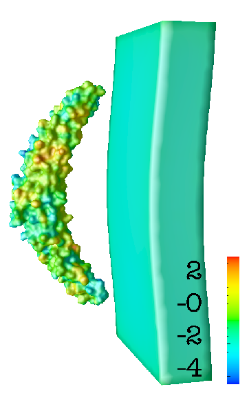


The dimer has a positively charged concave face and a net charge of . This negative net charge gives rise to a strong repulsive force to the negatively charged membrane surfaces when the ion screening is weak, which along with the repulsive dielectric pressure leads to a positive bending curvature of /Å. A transitional ion concentration is found at , below which the bending curvature is positive while above which the curvature is negative. Similar to the second model problem we tested above, this transitional ion concentration corresponds to the state in which the screened attractive interaction between the positively charged side of the dimer and the negatively charged membrane surfaces is balanced by the repulsive interaction between the negative charged side of the dimer and the membrane surfaces plus the dielectric pressure as well as the ionic pressure. The maximum curvature, /Å, occurs at an ion concentration of , while the curvature at the physiological concentration, in this study, is /Å. These demonstrate that the present model is able to capture the critical role of the mobile ions in mediating the protein-membrane interactions. Nevertheless, all these bending curvatures are smaller than the intrinsic curvature of the dimer (/Å). We speculate that a larger curvature could be found at suitable initial separation between the membrane and the dimer. However, the simulations with various separations (c.f. Fig. 3) illustrate that the bending curvature becomes slightly smaller as the separation gets smaller. These observations suggest that the attractive electrostatic force is not sufficiently strong to generate a bending curvature as large as the intrinsic curvature of the dimer when the membrane is constrained at two -ends. On the other hand, a charged membrane free of these constraints will move towards the dimer under the attraction and eventually contact with the two ends of the dimer; these two ends will then serve as the constraints for the bending of the membrane. This procedure has been observed in molecular dynamical simulations [6, 9], where the two ends of the dimer will insert into the membrane after contacting with the membrane and further facilitate the bending of the membrane.
The results clearly demonstrate that our continuum electromechanical model efficiently captures the balance between the electrostatic energy and the elastic strain energy in the protein-membrane interaction. The model quantitatively characterizes the dependence of the interaction on the solvation, partial charge distribution in protein, membrane composition and its surface charge distribution, and the membrane dielectric constant, some of which has been observed in previous studies [6, 9], but never described in a continuum framework. The present formalism is mainly limited by the fixed constraints on some un-charged membrane surfaces, which could be resolved by introducing the protein surface as a limit of membrane deformation [19]. Future efforts to improve these approximations are critical to accurately describe the protein-membrane interactions for more complicated geometries. The formulation and examples presented here are expected to spur the interests of other investigators in molecular biology, mechanics, and mathematics.
The authors thank Si Hang for the help with mesh generation. The research of YCZ is supported by Colorado State University. BZL is supported by the Chinese Academy of Sciences, the State Key Laboratory of Scientific/Engineering Computing, and NSFC(NSFC10971218). AAG acknowledges the support from the University of Texas Medical School at Houston.
References
- [1] A. J. Ridley, M. A. Schwartz, K. Burridge, R. A. Firtel, M. H. Ginsberg, G. Borisy, J. T. Parsons, and A. R. Horwitz, Science, 302, 1704 (2003).
- [2] W. Cho and R. V. Stahelin, 34, 119 (2005).
- [3] P. Wiggins and R. Phillips, Biophys. J., 88, 880 (2005).
- [4] B. J. Peter, H. M. Kent, I. G. Mills, Y. Vallis, P. J. G. Butler, P. R. Evans, and H. T. McMahon, Science, 303, 495 (2004).
- [5] S. Saksena, J. Sun, T. Chu, and S. D. Emr, Trends Biochem Sci., 32, 561 (2007).
- [6] P. D. Blood and G. A. Voth, Proc. Natl. Acad. Sci. U.S.A., 103, 15068 (2006).
- [7] D. K. Fygenson, J. F. Marko, and A. Libchaber, Phys. Rev. Lett., 79, 4497 (1997).
- [8] G. Fabrikant, S. Lata, J. D. Riches, J. A. G. Briggs, W. Weissenhorn, and M. M. Kozlov, PLoS Comput Biol, 5, e1000575 (2009).
- [9] A. Arkhipov, Y. Yin, and K. Schulten, Biophys. J., 95, 2806 (2008).
- [10] W. S. Klug, R. F. Bruinsma, J. P. Michel, C. M. Knobler, I. L. Ivanovska, C. F. Schmidt, and G. J. L. Wuite, Phys. Rev. Lett., 97, 228101 (2006).
- [11] K. A. Sharp and B. Honig, J. Phys. Chem., 94, 7684 (1990).
- [12] Y. Zhou, M. Holst, and J. A. McCammon, J. Math. Anal. Appl., 340, 135 (2008).
- [13] M. K. Gilson, M. E. Davis, B. A. Luty, and J. A. McCammon, J. Phys. Chem., 97, 3591 (1993).
- [14] B. Lu, M. J. Holst, J. A. McCammon, and Y. C. Zhou, J. Comput. Phys., 1, 1 (2010).
- [15] P. G. Ciarlet, Mathematical Elasticity Volume I: Three-dimensional elasticity (North-Holland, 1987).
- [16] A replicated system has a surface area Å2, each unit having 36 lipids in its monolayer. Only 30% of lipids have a unit negatively charged head group. The surface charge density is then .
- [17] Y. Tang, G. Cao, X. Chen, J. Yoo, A. Yethiraj, and Q. Cui, Biophys. J., 91, 1248 (2006).
- [18] B. Li, SIAM J. Math. Anal., 40, 2536 (2009).
- [19] N. Kikuchi and J. T. Oden, Contact Problems in Elasticity: A Study of Variational Inequalities and Finite Element Methods (SIAM, 1988).