: an Efficient Program for Genotype Elimination
Abstract
This paper presents an efficient program for checking Mendelian consistency in a pedigree. Since pedigrees may contain incomplete and/or erroneous information, geneticists need to pre-process them before performing linkage analysis. Removing superfluous genotypes that do not respect the Mendelian inheritance laws can speed up the linkage analysis. We have described in a formal way the Mendelian consistency problem and algorithms known in literature. The formalization helped to polish the algorithms and to find efficient data structures. The performance of the tool has been tested on a wide range of benchmarks. The results are promising if compared to other programs that treat Mendelian consistency.
keywords: abstract interpretation
1 Introduction
Geneticists employ the so-called linkage analysis to relate genotypic information with their corresponding phenotypic information. Genotypes are organized in data structures called pedigrees, that besides genetic data, record which individuals mate and their offspring. Since pedigrees may contain incomplete and/or erroneous information, geneticists need to pre-process them before performing linkage analysis. Moreover, in many cases, we cannot know any genetic information for some individuals (for instance because they refuse to or cannot be analyzed) and we would like to know which are their possible genotypes. Therefore, we would like to pre-process the pedigree by removing some candidate genotypes, in such a way that the remaining genotypes respect the classical Mendelian laws. When the pedigree is composed by thousands of individuals, this consistency checking need to be automated. The first notable contribution in the pedigree consistency check is the algorithm proposed by Lange and Goradia in 1987 [7]. The algorithm takes as input a pedigree with a list of genotypes associated to every individual, and perform genotypes elimination by removing from the lists the genotypes that lead to Mendelian inconsistencies. The algorithm performs a fixpoint iteration by processing one nuclear family at a time. This algorithm is optimal (in the sense that it removes all the genotypes that lead to Mendelian inconsistencies, and only them) when the pedigree has no loops. An example of loop in a pedigree is when two individuals that mate have an ancestor in common. An algorithm that is optimal even in the presence of loops has been proposed by O’Connell and Weeks in 1999 [9]. In brief, the algorithm selects the loop breakers (that is the individuals that, if duplicated, remove the loop) and perform the Lange Goradia algorithm for every combination of the genotypes of the loop breakers. Unfortunately, it has been proven [2] that the consistency check on pedigrees with marker data containing at least three alleles is a NP-hard problem.
The remainder of the paper is organized as follows. Firstly, we formalize the problem of genotype elimination (Section 2) and the algorithms of Lange-Goradia (Section 2.1) and O’Connell and Weeks (2.2). Then, we describe the implementation of (Section 3). Section 4 describes the performances of on a large set of benchmarks. Then, we compare our program with other existing software (Section 5). Finally, we conclude and suggest some directions for future works.
2 Mendelian consistency algorithms
A pedigree contains parental and genetic information about a set of individuals. Pedigrees are usually represented in a graphical way by drawing a circle for every female individual and a box for every male individual. Inside the circle (or the box) there can be some data regarding the individual (for instance genetic information, or affection status). Parental relations are represented by lines that connect to a node (the so called marriage node). Arrows depart from the marriage nodes to the children of the couple. In Figure 1 we report the graph of a pedigree composed by 11 individuals. For each individual, we report his/her identification number (id from now on) and his/her possible genotypes.
We collect the parental structure in a triple where is the set of individuals and and are two partial functions from into mapping a subset of individuals to their father and mother, respectively. The individuals that do not have parents in the pedigree are called founders. For the pedigree of Fig. 1, the founders are the individuals with id in .
We suppose that we are looking at a single locus. The possible alleles in the locus are in the set , ranged by uppercase case letters . Let be the set of unordered pairs of elements in . Since we consider the genotypes and as equivalent, the genotype of each individual will be an element of the set . A fully specified genetic map of a pedigree is an element of . We say that a fully specified map (fsmap from now on) is Mendelian if the genotypes of every non-founder individual is such that one of its allele is derived from the mother and the other from the father. It is often useful to check for Mendelian consistency in a subset of the individuals in the pedigree. Since the Mendelian conditions involve an individual and both his parents, it makes sense to consider those subsets that contain either both or none of the parents of each individual in the subset. Given a pedigree we say that is a regular subset of if, for each , we have that . Intersections and unions of regular subsets are again regular subsets. For instance, in the pedigree of Fig. 1, the set is an an example of a regular subset of the individuals.

We can also define a function that, given two genotypes, returns the set of Mendelian genotypes that can be generated by selecting one allele from each one. We have (remember that we use unordered pairs):
With the help of function , we can now express more precisely when a fsmap is Mendelian on a regular subset of individuals:
Definition 1 (Mendelian consistency).
Let be a pedigree and let be a regular subset of . The fully specified map is Mendelian on if and only if for every individual such that and , we have .
We say that an fsmap on a pedigree is Mendelian if it is Mendelian on . The reader can verify that the fsmap in Fig. 1 is Mendelian.
Since in general we do not know precisely the genotype of each individuals, only partially specified maps will be available. A partially specified map (psmap from now on) records for every individual of the pedigree the genotypes it may have according to our information (e.g. because we have collected some genetic data or we have observed the phenotype). A psmap is an element of the set . We can introduce a partial order relation on set . We say that map is more precise than or equal to map , and we write , if and only if, for every individual , . With an abuse of notation we identify any fully specified map with the partially specified map that maps to every individual . Thus we write to mean that, for every individual , . All psmaps such that for any describe an inconsistent situation where no possible assignment of genotypes is compatible with the available information. We identify all these psmaps and denote them by , the psmap that maps to all individuals in . We denote by the set obtained by this identification. The set is a complete lattice, with least upper bound given by pointwise union. The greatest lower bound is obtained in two steps: first, the pointwise intersection is computed; then, if any individual is mapped to in the previous step, the result is taken to be .
In psmaps we are interested in those genotypes, taken from the sets of each individual, that can be used to build a Mendelian fsmap.
Definition 2 (Consistent genotype).
Let be a pedigree and let be a regular subset of . Given a psmap and an individual , we say that genotype is consistent on iff there exists an fsmap with such that is Mendelian on .
A psmap is consistent on if all , for all , are consistent on .
A pedigree consistency algorithm can be seen as a function that takes a psmap and returns another psmap where some inconsistent genotypes have been removed. More precisely, we define function such that and is consistent on .
We say that a psmap on a pedigree is fixed on a set if is a singleton set for all .
Example 3.
Let be a non-founder in the pedigree and assume the psmap is fixed on . Thus and . Let us compute . Consider . If then , otherwise .
Let and be two regular subsets of . We may want to obtain from and , which may be simpler to compute. A candidate composition is , since this operation keeps the genotypes which are consistent on both and . However, in general, we only have , and the relation may be strict. Nonetheless, it can be easily seen that the equality holds whenever is fixed on .
A useful function in the definition of consistency check algorithms is function . Given any , is the set of all psmaps such that is equal to on and is fixed on . Thus, if , then for each we have a psmap such that for all and for all . If is a pedigree and is a psmap on it, we have the following relation for all (where is regular)
| (1) |


2.1 The Lange-Goradia algorithm
The idea of the Lange-Goradia algorithm is to remove all the genotypes of an individual that are inconsistent on any nuclear family to which belongs. This is accomplished by looking at one nuclear family at a time. Let be a psmap for a pedigree . If is a nuclear family where and are the parents and are the children, then each pair of genotypes in is examined in turn, checking that for all the children with . If this is the case, then , and all genotypes in for each children are consistent on . All genotypes that are not found to be consistent after all pairs of genotypes in have been examined are certainly inconsistent on and, thus, also inconsistent, so they can be safely removed. More formally, we can say that the algorithm computes (note that a nuclear family is a regular subset of ), which is equal to according to (1). For each , is computed as . This is equal to since is fixed on . Finally, is computed as in Example 3, for each .
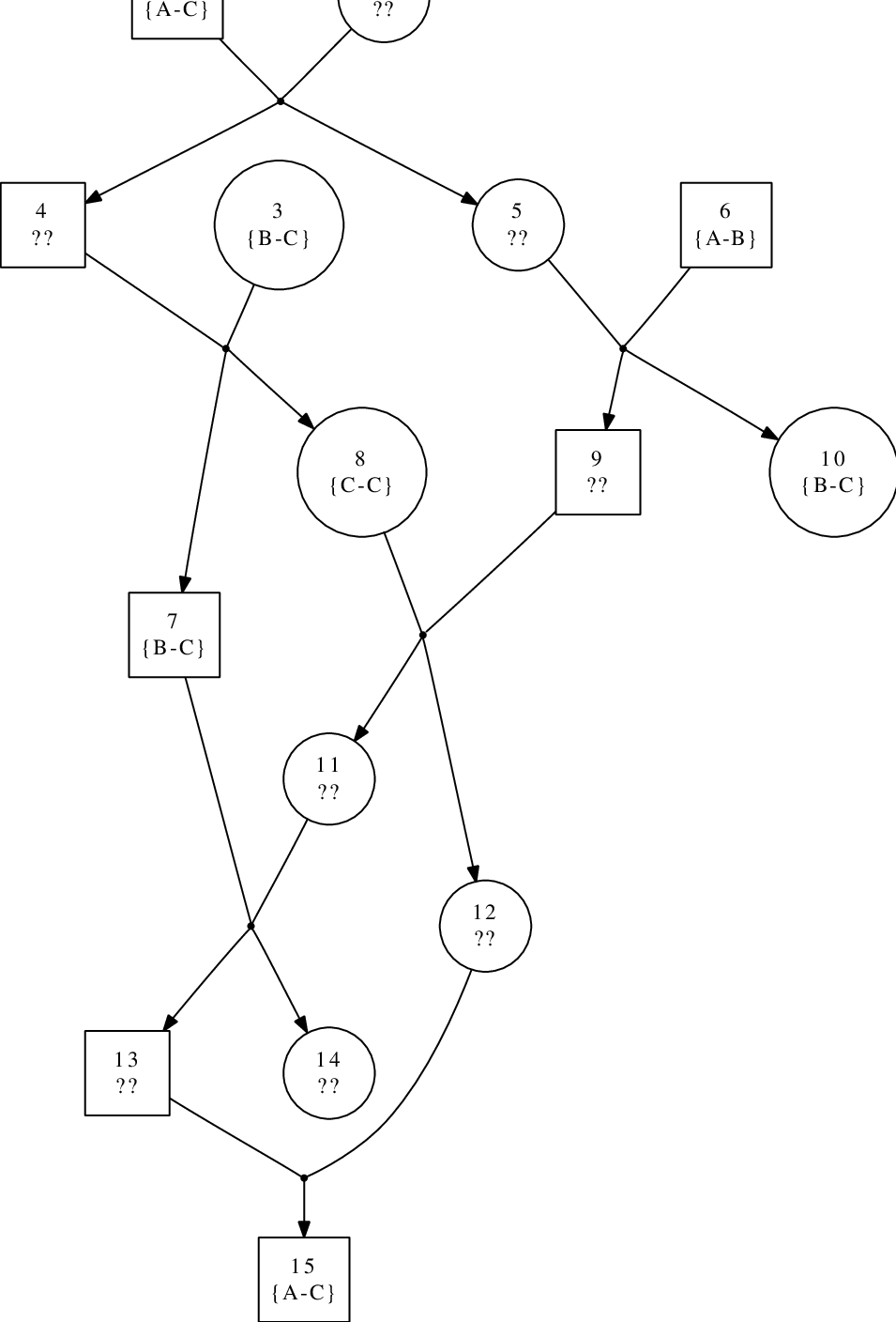
The algorithm is iterated on all nuclear families until no new genotypes are removed. If is the psmap obtained at the end of the algorithm and for any , then is consistent on all nuclear families to which belongs. Let us call the function that maps an input psmap to the output psmap according to the Lange-Goradia algorithm. In general, and the relation may be strict, i.e., the algorithm may not eliminate all inconsistent genotypes. As shown by Lange and Goradia [7], a sufficient condition for is the absence of loops in the pedigree. As an example, consider the pedigree of Figure 2. The pedigree contains loops, since there are individuals that mate that have an ancestor in common (for instance individuals 12 and 13 are both descendant of individual 8). Therefore, it is not guaranteed that the result of Lange-Goradia (Figure 2) contains only consistent genotypes. In fact, consider individual 9. Although the genotype is not consistent, the Lange-Goradia algorithm cannot eliminate it. To see that it is not possible to find a Mendelian fsmap that is of that depicted in Figure 2, consider individual 15. One of his alleles is . Since his alleles must come from individuals 7, 8, and 9, at least one of those individuals must have allele . Individuals 7 and 8 do not contain it, thus 9 must have as allele, and we can eliminate . We will see in the next subsection that the O’Connell and Weeks algorithm is able to eliminate from individual 9.
2.2 The O’Connell and Weeks algorithm
The O’Connell and Weeks algorithm [9] is able to remove all inconsistent genotypes from a psmap. The algorithm has the same input of the Lange-Goradia algorithm: a pedigree and a psmap . Let us call the function that maps an input psmap to the output psmap according to the O’Connell and Weeks algorithm.
First, a suitable set of loop breakers is found. A loop breaker is an individual that is involved in a loop in the pedigree and set must contain such an individual for each loop in the pedigree.
A new pedigree is built, where contains a new individual for each , is undefined for all , is equal to for all such that , and for all (and similarly for ). Thus, is obtained from by breaking all loops. Then, for each a psmap on is built, where for all and for all . Finally, is computed for all and all output psmaps thus obtained are joined. Since contains no loops, we have for all . It is easy to see that it is for all and that this implies that the restriction of to is consistent on . Indeed, if is the restriction of to we have .
We note that there is no need to actually build pedigree , since will produce the same result as whenever is fixed on . Thus we can simply define
| (2) |
For each we have , thus we obtain from (1).

Fig. 3 shows a block-diagram representation of the O’Connell and Weeks algorithm. Note that eq.(2) corresponds to the part of the diagram from the block onwards. The initial block is not necessary for the completeness of the algorithm, but is introduced in order to try to reduce the cost of the rest of the algorithm, since the number of Lange-Goradia invocations depends combinatorially on the number of genotypes assigned to each loop breaker.

As an example, consider the pedigree depicted in Figure 2. The pedigree contains various loops that can be broken, for instance, by choosing individuals 8 and 12 as loop breakers. This choice leads to three applications of the Lange-Goradia algorithm to the pedigree of Fig. 2 in which the individual 12 is typed as , , and , respectively. The three runs have as results the psmaps depicted in Figure 4. The union of these three psmaps gives as results the psmap depicted in Figure2. We can note that genotypes and have been eliminated from individual 9.
3 The tool
We have implemented the O’Connell and Weeks algorithm in a tool named . has been developed in C++ and is able to perform genotype elimination. Using a command-line switch, it is possible to select either Lange-Goradia or O’Connell and Weeks’s algorithm. receives as input a pedigree in pre-LINKAGE format, and writes the processed pedigree in a human-readable form. Moreover, it is also possible to have a DOT-file as output, that can be processed with Graphviz [4] to obtain a graphical representation of the resulting pedigree.
3.1 Parental information
In the design of our application, we kept the genotypic information separated from the parental information. During the parsing of the file, parental relations are stored in a redundant set of data structures (list of nuclear families in the pedigree, list of partners of each individual, list of families each individual belongs to, etc.). These data structures allow to recover all the parental relations needed by the consistency algorithms in a fast way. For instance, during the Lange-Goradia algorithm, to avoid unnecessary iterations, we set up a working list of the families to be processed. When the genotypes set of an individual changes, we insert in the working list only the families the individual belongs to.
3.2 Genotypes set as bitmaps
Our efficient implementation uses bitmaps to represent elements of (individual of a psmap). When the set contains few genotypes, a bitmap needs more space than other alternatives such as binary search trees. On the contrary, this slight drawback is counter-balanced by many advantages. First of all, the operations of search, insertion and deletion from subset of can be completed in constant time. Moreover, when the maximum number of alleles is known in advance, bitmaps can avoid the use of dynamic memory, thus speeding up the operations of copy and allocation/deallocation. Union and intersection of set of genotypes can be implemented with bitwise logical operations. Even the iteration of all the genotypes in a set can be implemented efficiently by calculating the least significant bit in a word.
We chose to represent alleles with unsigned integers in the range , where is the maximum number of alleles. With this choice, elements of are triangular bitmaps with rows. When , the -th word of the matrix represents the subset of composed by genotypes with as the first allele, and as the second allele. In this way, it is easy to build bit masks for manipulating sets of genotypes.
As an example, consider the optimization suggested in [9]. To
speed up the initial application of the Lange-Goradia algorithm, O’Connell and
Weeks suggest to pre-process the pedigree by removing those genotypes that can
be easily identified as superfluous by looking at a single parent-child pair. For
instance, when a child is fully specified with alleles , it is possible
to remove from its parents all the genotypes that do not contain at least one
from and . With the genotype set represented as a bitmap, it is
sufficient to clear all the bits that are not in words and in columns
. The C++ code of this operation can be found in Figure 5.
Concluding, the bitmap has been a key choice for speeding up all the consistency algorithms.
3.3 Loop breakers selection
We have seen that the O’Connell and Weeks algorithm executes the Lange-Goradia algorithm once for every combination of the genotypes of the loop breakers. Therefore, the selection of loop breakers greatly affects the total running time of the O’Connell and Weeks’s algorithm. In , we chose to apply the selection strategy suggested by Becker et al. [3]. The idea of the selection algorithm is to prefer to choose the individuals that break more loops at a time, and to avoid the ones that have a long list of genotypes. Becker et al. show that this problem is equivalent to the calculus of the minimum spanning tree of a directed graph. The graph to be analyzed can be obtained from the parental graph by removing all the individuals (and corresponding marriage nodes) that do not belong to any loop. This reduction of the graph must be put in place whenever a new loop breaker is chosen. The individuals in this graph are labelled with the result of a function that estimates the cost of the selection of the corresponding loop breaker. The function is defined as , where denotes the cardinality of set and is the number of neighbours of individual in the graph. The intended meaning of the function is to be a heuristic estimate of the number of loop the individual belongs to. We implemented the spanning tree calculus with a modified version of the classical algorithm by Kruskal [6]. In fact, in this case, the function (and in particular ) must be recalculated because the graph is reduced whenever a new loop breaker is found. However, since the cost of selection is only increasing, the greedy methodology of the spanning tree algorithm can be preserved.
It is easy to see that, by definition of , given and , with and fixed on , it holds . Therefore, in the phase, we discard all the loop breakers that have a single genotype.
3.4 Recursive vs non recursive reduction
To reduce the number of Lange-Goradia reductions (one for every combination of the genotypes of the loop breakers), O’Connell and Weeks suggest to use a recursive version of their algorithm. Instead of calculating all the combinations and applying the Lange-Goradia reduction, they adopt a backtracking methodology and execute a Lange-Goradia reduction whenever a loop breaker genotype is fixed. The algorithm can be expressed by the following pseudo-code. In the pseudo-code, given a function , we denote with the function defined as if , and otherwise. This notation is used for updating the
The rationale behind this approach is to avoid a brute-force exploration of the results of the function in (2). However, our experiments show that this approach does not pay off when coping with large pedigrees and few combinations to explore. In fact, all the psmaps that are on the recursion call stack must be initialized and copied, thus leading to an increased use of memory. When the number of individuals is not high and there are many combinations to explore, the recursive version is better than the non recursive one.
4 Performances of
We have tested with three different pedigrees. Following the methodology described in [11], we have simulated genetic data by picking founder alleles from the uniform distribution, applying randomly the Mendelian laws down the pedigree to calculate non-founder alleles, and, finally, deleting the genotype information of some individuals.
The first pedigree we considered is composed by 221 individuals. It is a human pedigree that traces the ancestors of two individuals affected by hypophosphatasia (HOPS). The pedigree comes from the Hutterite population living in North America, and it has been used previously in [8, 11].
We analyzed 100 datasets for each combination of the number of alleles (5, 7, 10, 12, 15, 17, 20, 25, 30), and of the ratio of untyped individual (5, 10, 20, 30, and 50 percent), for a total of 4500 datasets.
Then, we tested a larger pedigree composed by 4921 individuals. This pedigree was also studied in [11] and has been simulated with the method of Gasbarra et al. [5]. It has been used as a benchmark for the tool Allelic Path Explorer (APE). The pedigree contains 159 founders, and 75 percent of individuals were inbred. Again, simulating genetic data, we have created 100 datasets for each combination of number of alleles and each ratio of untyped individuals.
The last pedigree we tested is even bigger. It is composed by 8420 individuals and has been generated with the tool QMSIM [13]. It is composed of 10 generations. The founders are 420 individuals (400 females and 20 males). We have tested the performance of on a Intel Core 2 Duo 3.00 GHz machine equipped with 2GB of RAM and running Ubuntu Linux 9.10 (kernel version 2.6.31-21).
| Name | Individuals | Generations | %Founders | Avg Family size |
|---|---|---|---|---|
| HOPS | 221 | 12 | 21.72% | 1.52 |
| APE | 4921 | 15 | 3.23% | 1.82 |
| QMSIM | 8420 | 10 | 4.99% | 2.00 |
Figure 6 shows the execution time of when the Lange-Goradia algorithm is executed. We have put the number of alleles on the x axis and there is a line for every percentage of untyped individuals in the pedigree. Every dot in the graph refers to the average execution time of the 100 datasets for each combination number of alleles-ratio of untyped individual. We have used a logarithmic scale on the y axis, and therefore the linear trend corresponds to an exponential growth of the execution time when the number of alleles is raised. We can note that, even though the QMSIM pedigree is composed by a larger number of individuals than APE, the execution times are significantly lower. This could be due to its simple and regular parental structure (see Table 1 for a comparison). We have measured a very low variance among the same 100 datasets, except when the number of alleles is high and the percentage of untyped individual is set to 50%. This effect is particularly evident in benchmark APE. We reported in Figure 6 the mean, and the first three quartiles of the execution times of , when the ratio of untyped individuals is 50% and the alleles are between 20 and 30.


We have also tested the same benchmarks when executes the O’Connell and Weeks algorithm. However, in many cases, the loop breakers selection algorithm is able to find only loop breakers that have a single genotype. In this case, as we have seen in Section 3.3, the O’Connell and Weeks algorithm is equivalent to the Lange-Goradia. With a low rate of untyped individuals, the number of loop breakers (from now on we consider only the loop breakers with more than one genotype) is different from zero only in some sporadic cases, and thus the average execution time of the O’Connell and Weeks is very similar to the Lange-Goradia one (the only difference being the loop breaker selection procedure). We report in Table 2 the average number of loop breakers and the number of cases generated by the function. As shown in the table, there is the risk of a combinatorial explosion. When the ratio of unknown individuals has been set to 50%, we could not complete the O’Connell and Weeks analysis within 30 minutes of computations for 3 out of the 900 pedigrees of the HOPS benchmark and 8 out of 900 of the QMSIM benchmark, and for all the pedigrees of the APE benchmark.
| Benchmark | % unknown | Avg LB | Max LB | Avg Cases | Max Cases |
|---|---|---|---|---|---|
| HOPS | 50% | 0.0200 | 2 | 0.04 | 10 |
| 50% | 1.7622 | 10 | 686* | 4.66 | |
| QMSIM | 50% | 0.1175 | 6 | 0.18 | 240 |
| 50% | 2.6978 | 19 | 955* | 2.24 | |
| APE | 50% | 0.1175 | 4 | 0.19 | 32 |
| 50% | 8.398 | 172 | 4.02 | 3.61 |
In Figure 7 we have plotted the average executions of the O’Connell Weeks algorithm run on the benchmarks HOPS and QMSIM when only half of the individuals are typed. We can note that the recursive version of the algorithm dominates the non-recursive version. However, the gap between the twos is very small in QMSIM, due to the overhead of the backtracking procedure that nearly counter-balances the advantage of executing fewer Lange-Goradia iterations.


5 Comparison with other software
O’Connell and Weeks have implemented their algorithms in the Pedcheck program [10]. Pedcheck is able to check Mendelian consistency in pedigree with different levels of accuracy (and therefore with different computational requirements). Level 1 analysis is able to discover simple errors related to a single nuclear family (a child and parent’s alleles are incompatible, more than 4 alleles in a sibship, or 3 if there is a homozygous child). Level 2 correspond to Lange-Goradia algorithm. Level 3 and 4 provide a basic support to error correction. Level 3 identifies the so-called critical genotypes (that is the individuals that, if left untyped, make the pedigree consistent). Level 4 requires to know the frequencies of the alleles to estimate the most probable corrections.
At this time is more precise than Pedcheck as regards to genotype elimination, but it does not offer error correction capabilities. is more precise because it can also perform O’Connell and Weeks algorithm that we have seen is more precise than the Lange-Goradia algorithm. Moreover, when Pedcheck is applied to large pedigrees, even the Level 2 (Lange-Goradia) phase, takes a considerable amount of time. For example, consider the QMSIM benchmarks (8420 individuals and 4000 families). Even with only 10% of untyped individuals and 5 alleles, Pedcheck needs about 10 minutes of computation, while our program executes the Lange-Goradia algorithm in less than 20 milliseconds. We performed the same tests that we used on our tool and we found that Pedcheck could complete the analysis in times comparable with ours only on the HOPS benchmark . We report in Figure 8 the average execution times of (with the Lange-Goradia algorithm) and Pedcheck (level 2 analysis) for the HOPS benchmarks and ratio of untyped individuals varying from 10 to 50%. We can see that always outperforms Pedcheck.


Mendelsoft [12] is another tool that is able to check Mendelian consistency and perform error correction. Sanchez et al. model the Mendelian consistency problem with soft constraint networks and use a generic weighted constraint network (WCN) solver. In this way, they are not limited to a single error and can also correct pedigree with multiple errors. They evaluate their tool with random and real pedigrees composed of thousands of individuals and containing many errors. Even if we cannot directly compare Mendelsoft with (that does not have error correction capabilities), we can note that the memory requirements of the WCN solver are very high. We have tested Mendelsoft with a machine equipped with 2GB of RAM and in many cases the program crashed because the amount of virtual memory was not sufficient. In particular, for the HOPS pedigree, Mendelsoft do not complete with this amount of RAM when the number of alleles is above 12.
6 Conclusions and future works
We have described the design and implementation of , a program that performs genotype elimination. The design of the program has been aided by a formal description of the problem that highlighted the critical aspects of the algorithms and helped us to find the best data structures. We have measured the performances of the program and we have found that is able to cope with large pedigrees. In the future, we would like to improve the working list selection algorithm of the Lange-Goradia elimination procedure and to test different loop breakers selection algorithms on highly-looped pedigrees, such as the one found in the APE test cases.
References
- [2] Luca Aceto, Jens A. Hansen, Anna Ingólfsdóttir, Jacob Johnsen & John Knudsen (2004): The complexity of checking consistency of pedigree information and related problems. J. Comput. Sci. Technol. 19(1), pp. 42–59.
- [3] Ann Becker, Dan Geiger & Alejandro A Schäffer (1998): Automatic selection of loop breakers for genetic linkage analysis. Human heredity 48(1).
- [4] J. Ellson, E.R. Gansner, E. Koutsofios, S.C. North & G. Woodhull (2003): Graphviz and Dynagraph – Static and Dynamic Graph Drawing Tools. In: M. Junger & P. Mutzel, editors: Graph Drawing Software, Springer-Verlag, pp. 127–148.
- [5] Dario Gasbarra, Mikko J. Sillanpää & Elja Arjas (2005): Backward simulation of ancestors of sampled individuals. Theoretical Population Biology 67(2), pp. 75 – 83. Available at http://www.sciencedirect.com/science/article/B6WXD-4F6F67C-1/%2/134b19fb4e742340bb5b97813e0308b8.
- [6] Jr. Kruskal, Joseph B. (1956): On the Shortest Spanning Subtree of a Graph and the Traveling Salesman Problem. Proceedings of the American Mathematical Society 7(1), pp. 48–50. Available at http://www.jstor.org/stable/2033241.
- [7] K. Lange & T.M. Goradia (1987): An Algorithm for Automatic Genotype Elimination. Am. J. Human Genetics 40, pp. 250–256.
- [8] Y. Luo & S. Lin (2003): Finding starting points for Markov chain Monte Carlo analysis of genetic data from large and complex pedigrees. Genet. Epidemiol. 25(1), pp. 14–24.
- [9] J. R. O’Connell & D. E. Weeks (1999): An optimal algorithm for automatic genotype elimination. Am. J. Human Genetics 65(6), pp. 1733–1740.
- [10] Jeffrey R. O’Connell & Daniel E. Weeks (1998): PedCheck: A Program for Identification of Genotype Incompatibilities in Linkage Analysis. The American Journal of Human Genetics 63(1), pp. 259 – 266. Available at http://www.sciencedirect.com/science/article/B8JDD-4R1WP1V-17%/2/b556d7a79c50d44c4f200e65a4eac506.
- [11] Matti Pirinen & Dario Gasbarra (2006): Finding Consistent Gene Transmission Patterns on Large and Complex Pedigrees. IEEE/ACM Trans. Comput. Biol. Bioinformatics 3(3), pp. 252–262.
- [12] Marti Sanchez, Simon Givry & Thomas Schiex (2008): Mendelian Error Detection in Complex Pedigrees Using Weighted Constraint Satisfaction Techniques. Constraints 13(1-2), pp. 130–154.
- [13] Mehdi Sargolzaei & Flavio S. Schenkel (2009): QMSim: a large-scale genome simulator for livestock. Bioinformatics 25(5), pp. 680–681. Available at http://dx.doi.org/10.1093/bioinformatics/btp045.