跳到论文正文
W Papers独立论文阅读器 arXiv:1008.2923 论文正文 计算阅读时间 · 0%
引用这篇论文根据当前论文元数据生成,正式投稿前建议核对。


License: arXiv.org perpetual non-exclusive license
arXiv:1008.2923v4 [math.SP] 03 Nov 2011

A Spectral Theory for Tensors

Edinah K. Gnang ††thanks: Department of Computer Science, Rutgers University, Piscataway, NJ 08854-8019 USA    Ahmed Elgammal ††thanks: Department of Computer Science, Rutgers University, Piscataway, NJ 08854-8019 USA    Vladimir Retakh ††thanks: Department of Mathematics, Rutgers University, Piscataway, NJ 08854-8019 USA
Abstract

In this paper we propose a general spectral theory for tensors. Our proposed factorization decomposes a tensor into a product of orthogonal and scaling tensors. At the same time, our factorization yields an expansion of a tensor as a summation of outer products of lower order tensors. Our proposed factorization shows the relationship between the eigen-objects and the generalised characteristic polynomials. Our framework is based on a consistent multilinear algebra which explains how to generalise the notion of matrix hermicity, matrix transpose, and most importantly the notion of orthogonality. Our proposed factorization for a tensor in terms of lower order tensors can be recursively applied so as to naturally induces a spectral hierarchy for tensors.

1 Introduction

In 1762 Joseph Louis Lagrange formulated what is now known as the eigenvalue - eigenvector problem, which turns out to be of significant importance in the understanding several phenomena in applied mathematics as well as in optimization theory. The spectral theory for matrices is widely used in many scientific and engineering domains.

In many scientific domains, data are presented in the form of tuples or groups, which naturally give rise to tensors. Therefore, the generalization of the eigenvalue-eigenvector problem for tensors is a fundamental question with broad potential applications. Many researchers suggested different forms of tensor decompositions to generalize the concepts of eigenvalue-eigenvector and Singular Value Decomposition.

In this paper we propose a mathematical framework for high-order tensors algebra based on a high-order product operator. This algebra allows us to generalize familiar notions and operations from linear algebra including dot product, matrix adjoints, hermicity, permutation matrices, and most importantly the notion of orthogonality. Our principal result is to establish a rigorous formulation of tensor spectral decomposition through the general spectral theorem. We prove the spectral theorem for hermitian finite order tensors with norm different from 11. Finally we point out that one of the fundamental consequence of the spectral theorem is the existence of a spectral hierarchy which determines a given hermitian tensor of finite order.

There are certain properties that a general spectral theory is expected to satisfy. The most fundamental property one should expect from a general formulation of the spectral theorem for tensors is a factorization of a cubic tensor into a certain number of cubic tensors of the same dimensions. Our proposed factorization decomposes a Hermitian tensor into a product of orthogonal and scaling tensors. Our proposed factorization also extends to handle non-Hermitian tensors. Furthermore our proposed factorization offers an expansion of a tensor as a summation of lower order tensors that are obtained through outer products. Our proposed factorization makes an explicit connection between the eigen-objects and the reduced set of characteristic polynomials. The proposed framework describes the spectral hierarchy associated with a tensor. Finally the framework aims to extend linear algebraic problems found in many domains to higher degree algebraic formulations of corresponding problems.

The organization of this paper is as follows; Section [2] reviews the state of the art in tensor decomposition and its relation to the proposed formulation. Section [3] introduces our proposed tensor algebra for order three tensors. Section [4] introduces and proves our proposed spectral theorem for order three tensors. Section [5] discusses some important properties following from the proposed spectral decomposition. Section [6] proposes a computational framework for describing the characteristic polynomials of a tensor. Section [7] generalizes the introduced concepts to higher order tensors and introduces the notion of the spectral hierarchy. Section [8] discusses in details the relation between the proposed framework and some existing tensor decomposition frameworks. Section [9] concludes the paper with a discussion on the open directions.

2 State of the art in tensor decomposition

2.1 Generalizing Concepts from Linear Algebra

In this section we recall the commonly used notation by the multilinear algebra community where a kk-tensor denotes a multi-way array with kk indices [17]. Therefore, a vector is a 11-tensor and a matrix is a 22-tensor. A 33-tensor 𝑨\boldsymbol{A} of dimensions m×n×pm\times n\times p denotes a rectangular cuboid array of numbers. The array consists of mm rows, nn columns, and pp depths with the entry ai,j,ka_{i,j,k} occupying the position where the it​hi^{th} row, the jt​hj^{th} column, and the kt​hk^{th}depth meet. For many purposes it will suffice to write

𝑨=(ai,j,k)(1≤i≤m; 1≤j≤n; 1≤k≤p),\boldsymbol{A}=\left(a_{i,j,k}\right)\;\left(1\leq i\leq m;\,1\leq j\leq n;\,1\leq k\leq p\right), (1)

we now introduce generalizations of complex conjugate and inner product operators.
The order pp conjugates of a scalar complex number zz are defined by:

z𝔠pj≡ℜ2⁡(z)+ℑ2⁡(z)​exp⁡{i×arctan⁡{ℑ⁡(z)ℜ⁡(z)}×exp⁡{i​2​π​jp}}z^{\mathfrak{c}_{p}^{j}}\equiv\sqrt{\Re^{2}\left(z\right)+\Im^{2}\left(z\right)}\;\exp\left\{i\times\arctan\left\{\frac{\Im\left(z\right)}{\Re\left(z\right)}\right\}\times\exp\left\{i\frac{2\pi\,j}{p}\right\}\right\} (2)

where ℑ⁡(z)\Im\left(z\right) and ℜ⁡(z)\Re\left(z\right) respectively refer to the imaginary and real part of the complex number zz, equivalently rewritten as

z𝔠pj≡|z|​exp⁡{i×∠z×exp⁡{i​2​π​jp}},z^{\mathfrak{c}_{p}^{j}}\equiv\left|z\right|\exp\left\{i\times\angle_{z}\times\exp\left\{i\frac{2\pi\,j}{p}\right\}\right\}, (3)

from which it follows that

|z|p=∏1≤j≤pz𝔠pj.\left|z\right|^{p}=\prod_{1\leq j\leq p}z^{\mathfrak{c}_{p}^{j}}\>. (4)

The particular inner product operator that we introduce relates the inner product of a pp-tuple of vectors in ℂl\mathbb{C}^{l} to a particular ℓp\ell_{p} norm operator ℂl\mathbb{C}^{l} in a way quite similar to the way the inner product of pairs of vectors relate to the usual ℓ2\ell_{2} vector norm. We refer to the norm operator ‖‖ℓp:ℂl→ℝ+\left\|\>\right\|_{\ell_{p}}:\mathbb{C}^{l}\rightarrow\mathbb{R}^{+} (for every integer p≥2p\geq 2) as the ℓp\ell_{p} norm defined for an arbitrary vector 𝒙≡(x⁡(1),⋯,x⁡(l))∈ℂl\boldsymbol{x}\equiv\left(\begin{array}[]{ccc}x(1),&\cdots,&x(l)\end{array}\right)\in\mathbb{C}^{l} by

‖𝒙‖ℓp≡[∑1≤k≤l∏1≤j≤p(x⁡(k))𝔠pp−j]1p,\left\|\boldsymbol{x}\right\|_{\ell_{p}}\equiv\left[\sum_{1\leq k\leq l}\;\prod_{1\leq j\leq p}\left(x(k)\right)^{\mathfrak{c}_{p}^{p-j}}\right]^{\frac{1}{p}}, (5)

the inner product operator for a pp-tuple of vectors in ℂl\mathbb{C}^{l} denoted ⟨⟩:(ℂl)p→ℂ\left\langle\;\right\rangle:\;\left(\mathbb{C}^{l}\right)^{p}\rightarrow\mathbb{C} is defined by

⟨𝒗k⟩0≤k≤p≡∑1≤j≤l{∏0≤k≤p−1(vk​(j))𝔠pp−j}\left\langle\boldsymbol{v}_{k}\right\rangle_{0\leq k\leq p}\equiv\sum_{1\leq j\leq l}\left\{\prod_{0\leq k\leq p-1}\left(v_{k}(j)\right)^{\mathfrak{c}_{p}^{p-j}}\right\} (6)

some of the usual properties of inner products follow from the definition

⟨(𝒙1+𝒚1);𝒛2;⋯;𝒛l⟩=⟨𝒙1;𝒛2;⋯;𝒛l⟩+⟨𝒚1;𝒛2;⋯;𝒛l⟩\left\langle\left(\boldsymbol{x}_{1}+\boldsymbol{y}_{1}\right)\,;\,\boldsymbol{z}_{2}\,;\,\cdots\,;\,\boldsymbol{z}_{l}\right\rangle=\left\langle\boldsymbol{x}_{1}\,;\,\boldsymbol{z}_{2}\,;\,\cdots\,;\,\boldsymbol{z}_{l}\right\rangle+\left\langle\boldsymbol{y}_{1}\,;\,\boldsymbol{z}_{2}\,;\,\cdots\,;\,\boldsymbol{z}_{l}\right\rangle (7)

and most importantly the fact that

⟨𝒛;𝒛;⋯;𝒛;𝒛⏟p​o​p​e​r​a​n​d​s⟩≥0\left\langle\underbrace{\boldsymbol{z}\,;\,\boldsymbol{z}\,;\,\cdots\,;\,\boldsymbol{z}\,;\,\boldsymbol{z}}_{p\>operands}\right\rangle\geq 0 (8)

and

⟨𝒛;𝒛;⋯;𝒛;𝒛⏟p​o​p​e​r​a​n​d​s⟩=0⇔𝒛=𝟎.\left\langle\underbrace{\boldsymbol{z}\,;\,\boldsymbol{z}\,;\,\cdots\,;\,\boldsymbol{z}\,;\,\boldsymbol{z}}_{p\>operands}\right\rangle=0\Leftrightarrow\boldsymbol{z}=\boldsymbol{0}. (9)

We point out that the definitions of inner products is extended naturally to tensors as illustrated bellow

⟨𝑨,𝑩⟩≡∑1≤m,n≤lam,n×(bn,m)𝔠21\left\langle\boldsymbol{A},\boldsymbol{B}\right\rangle\equiv\sum_{1\leq m,n\leq l}a_{m,n}\times\left(b_{n,m}\right)^{\mathfrak{c}_{2}^{1}} (10)
⟨𝑨,𝑩,𝑪⟩≡∑1≤m,n,p≤lam,n,p×(bp,m,n)𝔠32×(cn,p,m)𝔠31,\left\langle\boldsymbol{A},\boldsymbol{B},\boldsymbol{C}\right\rangle\equiv\sum_{1\leq m,n,p\leq l}a_{m,n,p}\times\left(b_{p,m,n}\right)^{\mathfrak{c}_{3}^{2}}\times\left(c_{n,p,m}\right)^{\mathfrak{c}_{3}^{1}}, (11)

More generally for arbitrarly finite order tensor the inner product for the family of tensors {𝑨(t)=(ai1,i2,⋯,in(t))}1≤t≤n\left\{\boldsymbol{A}^{(t)}=\left(a_{i_{1},i_{2},\cdots,i_{n}}^{(t)}\right)\right\}_{1\leq t\leq n} is defined by:

⟨𝑨(t)⟩1≤t≤n≡∑1≤i1,i2,⋯,in≤l(∏0≤t≤n−1(ai1+(t−1),⋯,in+(t−1)(t))𝔠np−t)\left\langle\boldsymbol{A}^{(t)}\right\rangle_{1\leq t\leq n}\equiv\sum_{1\leq i_{1},i_{2},\cdots,i_{n}\leq l}\left(\prod_{0\leq t\leq n-1}\left(a_{i_{1+\left(t-1\right)},\cdots,i_{n+\left(t-1\right)}}^{(t)}\right)^{\mathfrak{c}_{n}^{p-t}}\right) (12)

note that the addition in the indices are performed modulo nn.
Generalization of other concepts arising from linear algebra have been investigated quite extensively in the literature. Cayley in [1] instigated investigations on hyperdeterminants as a generalization of determinants. Gelfand, Kapranov and Zelevinsky followed up on Cayley’s work on the subject of hyperdeterminants by relating hyperdeterminants to XX-discriminants in their book [10].
A recent approach for generalizing the concept of eigenvalue and eigenvector has been proposed by Liqun Qi in [30, 28] and followed up on by Lek-Heng Lim[26], Cartwright and Sturmfels [5]. The starting point for their approach will be briefly summarized using the notation introduced in the book [10]. Assuming a choice of a coordinate system 𝒙j=(xj​(0),xj​(1),⋯,xj​(kj))\boldsymbol{x}_{j}=\left(x_{j}(0),x_{j}(1),\cdots,x_{j}(k_{j})\right) associated with each one of the vector space Vj≡(ℝ+)kj+1V_{j}\equiv\left(\mathbb{R}^{+}\right)^{k_{j}+1}. We consider a multilinear function f:⨂t=1rVt→ℝ+f\>:\;\bigotimes_{t=1}^{r}V_{t}\rightarrow\mathbb{R}^{+} expressed by :

f(𝒙1,𝒙2,⋯,𝒙r−1,𝒙r)=∑i1,⋯,irai1,⋯,irx1(i1)⋯xr(ir),f\left(\boldsymbol{x}_{1},\boldsymbol{x}_{2},\cdots,\boldsymbol{x}_{r-1},\boldsymbol{x}_{r}\right)=\sum_{i_{1},\cdots,i_{r}}a_{i_{1},\cdots,i_{r}}x_{1}(i_{1})\cdots x_{r}(i_{r}), (13)

equivalently the expression above can be rewritten as

f⁡(𝒙1,𝒙2,⋯,𝒙r−1,𝒙r)≡⟨𝒙1,𝒙2,⋯,𝒙r−1,𝒙r⟩𝑨.f\left(\boldsymbol{x}_{1},\boldsymbol{x}_{2},\cdots,\boldsymbol{x}_{r-1},\boldsymbol{x}_{r}\right)\equiv\left\langle\boldsymbol{x}_{1},\boldsymbol{x}_{2},\cdots,\boldsymbol{x}_{r-1},\boldsymbol{x}_{r}\right\rangle_{\boldsymbol{A}}. (14)

which of course is a natural generalization of bilinear forms associated with a matrix representation of a linear map for some choice of coordinate system

f⁡(𝒙1,𝒙2)=∑i1,i2ai1,i2​x1​(i1)​x2​(i2)≡(𝒙1)T​𝑨​𝒙1≡⟨𝒙1,𝒙2⟩𝑨.f\left(\boldsymbol{x}_{1},\boldsymbol{x}_{2}\right)=\sum_{i_{1},i_{2}}a_{i_{1},i_{2}}\>x_{1}(i_{1})\,x_{2}(i_{2})\equiv\left(\boldsymbol{x}_{1}\right)^{T}\boldsymbol{A}\>\boldsymbol{x}_{1}\equiv\left\langle\boldsymbol{x}_{1},\boldsymbol{x}_{2}\right\rangle_{\boldsymbol{A}}. (15)

It follows from the definition of the multilinear function ff that the function induces rr not necessarily distinct multilinear projective maps denoted by fk:⨂t=1t≠krVt→Vkf_{k}:\;\bigotimes_{\begin{array}[]{c}t=1\\ t\neq k\end{array}}^{r}V_{t}\rightarrow V_{k} expressed as :

fk(𝒙1,𝒙2,⋯𝒙k−1,𝒙k+1,⋯,𝒙r)=∑i1,⋯,ik−1,ik+1⋯,irai1,⋯,irx1(i1)x2(i2)⋯xk−1(ik−1)xk+1(ik+1)⋯xr(ir)f_{k}\left(\boldsymbol{x}_{1},\boldsymbol{x}_{2},\cdots\boldsymbol{x}_{k-1},\boldsymbol{x}_{k+1},\cdots,\boldsymbol{x}_{r}\right)=\sum_{i_{1},\cdots,i_{k-1},i_{k+1}\cdots,i_{r}}a_{i_{1},\cdots,i_{r}}x_{1}(i_{1})\,x_{2}(i_{2})\cdots\>x_{k-1}(i_{k-1})\>x_{k+1}(i_{k+1})\cdots\,x_{r}(i_{r}) (16)

The various formulations of eigenvalue eigenvector problems as proposed and studied in [30, 28, 5, 26] arise from investigating solutions to equations of the form:

fk​(𝒙,⋯,𝒙)=λ⋅𝒙f_{k}\left(\boldsymbol{x},\cdots,\boldsymbol{x}\right)=\lambda\cdot\boldsymbol{x} (17)

Applying symmetry arguments to the tensor 𝑨\boldsymbol{A} greatly reduces the number of map fkf_{k} induced by 𝑨\boldsymbol{A}. For instance if 𝑨\boldsymbol{A} is supersymmetric (that is 𝑨\boldsymbol{A} is invariant under any permutation of it’s indices) then 𝑨\boldsymbol{A} induces a single map. Furthermore, different constraints on the solution eigenvectors 𝒙k\boldsymbol{x}_{k} distinguishes the EE-eigenvectors from the HH-eigenvectors and the ZZ-eigenvectors as introduced and discussed in [30, 28].

Our treatment considerably differs from the approaches described above in the fact that our aim is to find a decomposition for a given tensor 𝑨\boldsymbol{A} that provides a natural generalization for the concepts of Hermitian and orthogonal matrices. Furthermore our approach is not limited to supersymmetric tensors.

In connection with our investigations in the current work, we point out another concepts from linear algebra for which the generalization to tensor plays a significant role in complexity theory, that is the notion of matrix rank. Indeed one may also find an extensive discussions on the topic of tensor rank in [29, 13, 15, 31, 6]. The tensor rank problem is perhaps best described by the following optimization problem. Given an rr-tensor 𝑨=(ai1,⋯,ir)\boldsymbol{A}=\left(a_{i_{1},\cdots,i_{r}}\right) we seek to solve the following problem which attempts to find an approximation of 𝑨\boldsymbol{A} as a linear combination of rank one tensors.

min(⊗𝒙k(t))1≤t≤r∈(⨂1≤t≤rVt)‖(∑1≤k≤l(λk)r⨂1≤t≤r𝒙k(t))−𝑨‖\min_{\left(\otimes\boldsymbol{x}_{k}^{(t)}\right)_{1\leq t\leq r}\in\left(\bigotimes_{1\leq t\leq r}V_{t}\right)}\left\|\left(\sum_{1\leq k\leq l}\left(\lambda_{k}\right)^{r}\bigotimes_{1\leq t\leq r}\boldsymbol{x}_{k}^{(t)}\right)-\boldsymbol{A}\right\| (18)

Our proposed tensor decomposition into lower order tensors relates to the tensor rank problem but differs in the fact that the lower order tensors arising from the spectral decomposition of 33-tensors, named eigen-matrices are not necessarily rank 11 matrices.

2.2 Existing Tensor Decomposition Framework

Several approaches have been introduced for decomposing kk-tensors for k≥3k\geq 3 in a way inspired by matrix SVD. SVD decomposes a matrix 𝑨\boldsymbol{A} into 𝑨=𝑼​𝚺​𝑽T\boldsymbol{A}=\boldsymbol{U}\boldsymbol{\Sigma}\boldsymbol{V}^{T} and can be viewed as a decomposition of the matrix 𝑨\boldsymbol{A} into a summation of rank-1 matrices that can be written as

𝑨=∑i=1rσi⊗(ui,vi)\boldsymbol{A}=\sum_{i=1}^{r}\sigma_{i}\;\otimes(u_{i},v_{i}) (19)

where rr is the rank of 𝑨\boldsymbol{A}, ui,viu_{i},v_{i} are the ii-th columns of the orthogonal matrices 𝑼\boldsymbol{U} and 𝑽\boldsymbol{V}, and σi\sigma_{i}’s are the diagonal elements of 𝚺\boldsymbol{\Sigma}, i.e., the singular values. Here ⊗(⋅,⋅)\otimes(\cdot,\cdot) denotes the outer product. The Canonical and Parallel factor decomposition (CANECOMP-PARAFAC, also caller the CP model), independently introduced by [4, 14], generalize the SVD by factorizing a tensor into a linear combination of rank-1 tensors. That is given 𝑨∈ℝn1×n2×n3\boldsymbol{A}\in\mathbb{R}^{n_{1}\times n_{2}\times n_{3}}, the goal is to find matrices 𝑼∈ℝn1×n1\boldsymbol{U}\in\mathbb{R}^{n_{1}\times n_{1}}, 𝑽∈ℝn2×n2\boldsymbol{V}\in\mathbb{R}^{n_{2}\times n_{2}} and 𝑾∈ℝn3×n3\boldsymbol{W}\in\mathbb{R}^{n_{3}\times n_{3}} such that

𝑨=∑i=1rσi⊗(ui,vi,wi)\boldsymbol{A}=\sum_{i=1}^{r}\sigma_{i}\;\otimes(u_{i},v_{i},w_{i}) (20)

where the expansion is in terms of the outer product of vectors ui,vi,wiu_{i},v_{i},w_{i} are the i-th columns of 𝑼\boldsymbol{U}, 𝑽\boldsymbol{V}, and 𝑾\boldsymbol{W}, which yields rank-1 tensors. The rank of 𝑨\boldsymbol{A} is defined as the minimum rr required for such an expansion. Here there are no assumption about the orthogonality of the column vectors of 𝑼\boldsymbol{U}, 𝑽\boldsymbol{V}, and 𝑾\boldsymbol{W}. The CP decomposition have been show to be useful in several applications where such orthogonality is not required. There are no known closed-form solution to determine the rank rr, or to find a lower rank approximation as given directly by matrix SVD.

Tucker decomposition, introduced in [34], generalizes over Eq 20, where an (n1×n2×n3)\left(n_{1}\times n_{2}\times n_{3}\right) tensor 𝑨\boldsymbol{A} is decomposed into rank-1 tensor expansion in the form

𝑨=∑i=1n1∑j=1n2∑k=1n3σi,j,k⊗(ui,vj,wk)\boldsymbol{A}=\sum_{i=1}^{n_{1}}\sum_{j=1}^{n_{2}}\sum_{k=1}^{n_{3}}\sigma_{i,j,k}\;\otimes(u_{i},v_{j},w_{k}) (21)

where ui∈ℝn1u_{i}\in\mathbb{R}^{n_{1}}, vj∈ℝn2v_{j}\in\mathbb{R}^{n_{2}}, and wk∈ℝn3w_{k}\in\mathbb{R}^{n_{3}}. The coefficients σi,j,k\sigma_{i,j,k} form a tensor that is called the core tensor 𝑪\boldsymbol{C}. It can be easily seen that if such core tensor is diagonal, i.e., σi,j,k=0\sigma_{i,j,k}=0 unless i=j=ki=j=k, Tucker decomposition reduces to the CP decomposition in Eq 20.

Orthogonality is not assumed in Tucker decomposition. Orthogonality constraints can be added by requiring ui,vj,wku_{i},v_{j},w_{k} to be columns of orthogonal matrices 𝑼\boldsymbol{U},𝑽\boldsymbol{V}, and 𝑾\boldsymbol{W}. Such decomposition was introduced in [21] and was denoted by High Order Singular Value Decomposition (HOSVD). Tucker decomposition can be written using the mode-nn tensor-matrix multiplication defined in [21] as

𝑨=𝑪×1𝑼×2𝑽×3𝑾\boldsymbol{A}=\boldsymbol{C}\times_{1}\boldsymbol{U}\times_{2}\boldsymbol{V}\times_{3}\boldsymbol{W} (22)

where ×n\times_{n} is the mode-nn tensor-matrix multiplication. Similar to Tucker decomposition, the core tensor of HOSVD is a dense tensor. However, such a core tensor satisfies an all-orthogonality property between its slices across different dimensions as defined in [21].

HOSVD of a tensor can be computed by flattening the tensor into matrices across different dimensions and using SVD on each matrix. Truncated version of the expansion yields a lower rank approximation of a tensor [22]. Several approaches have been introduced for obtaining lower rank approximation by solving a least square problem, e.g. [39]. Recently an extension to Tucker decomposition with non-negativity constraint was introduced with many successful applications [32].

All the above mentioned decompositions factorizes a high order tensor as a summation of rank-1 tensors of the same dimension, which is inspired by such an interpretation of matrix SVD as in Eq 19. However, none of these decomposition approaches can describe a tensor as a product of tensors as would be expected from an SVD generalization. The only known approach to us for decomposing a tensor to a product of tensors was introduced in a technical report [16]. This approach is based on the idea that a diagonalization of a circulant matrix can be obtained by Discrete Fourier Transform (DFT). Given a tensor, it is flattened then a block diagonal matrix is constructed by DFT of the circulant matrix formed from the flattened tensor. Matrix SVD is then used on each of the diagonal blocks. The inverse process is then used to put back the resulting decompositions into tensors. This approach results in a decomposition in the form 𝑨=𝑼⋆𝑺⋆𝑽T\boldsymbol{A}=\boldsymbol{U}\star\boldsymbol{S}\star\boldsymbol{V}^{T} where the product is defined as [16]

𝑨⋆𝑩=𝚏𝚘𝚕𝚍(circ(𝚞𝚗𝚏𝚘𝚕𝚍(𝑨,1)).𝚞𝚗𝚏𝚘𝚕𝚍(𝑩,1),1)\boldsymbol{A}\star\boldsymbol{B}=\mathtt{fold}(circ(\mathtt{unfold}(\boldsymbol{A},1)).\mathtt{unfold}(\boldsymbol{B},1),1)

However, such decomposition does not admit a representation of the decomposition into an expansion in terms of rank-1 tensors. The product is mainly defined by folding and unfolding the tensor into matrices.

From the above discussion we can highlight some fundamental limitations of the known tensor decomposition frameworks. Existing tensor decomposition frameworks are mainly expansions of a tensor as a linear combination of rank-1 tensors, which are the outer products of vectors under certain constraints (orthogonality, etc.) and do not provide a factorization into product of tensors of the same dimensions. Tucker decomposition, although a generalization of SVD, falls short of generalizing the notion of the spectrum for high-order tensors. There is no connection between the singular values and the spectrum of the corresponding cubic Hermitian tensors. Unfortunately, no such relation is proposed by the Tucker factorization. The Tucker decomposition does not suggest at all how to generalize such objects as the trace and the determinant of higher order tensors. In the appendix of this paper we show that Tucker decomposition and HOSVD uses notion of matrix orthogonality.

2.3 Applications of tensor decomposition

The most widely used formulation for tensor decomposition is the orthogonal version of Tucker decomposition (HOSVD) [21]. HOSVD is a multilinear rank revealing procedure [21, 22] and therefore, it has been widely used recently in many domains for dimensionality reduction and to estimate signal subspaces of tensorial data [18]. In computer vision, HOSVD has been used in [37, 38] for analysis of face images with different sources of variability, e.g. different people, illumination, head poses, expressions, etc. It has been also used in texture analysis, compression, motion analysis [35, 36], posture estimation, gait biometric analysis, facial expression analysis and synthesis, e.g. [9, 24, 23, 25], and other useful applications [18]. HOSVD decomposition gives a natural way for dealing with images as matrices [39]. The relation between HOSVD and independent component analysis ICA was also demonstrated in [7] with applications in communication, image processing, and others. Beyond vision and image processing, HOSVD has also been used in data mining, web search, e.g. [20, 19, 33], and in DNA microarray analysis [18].

3 33-tensor algebra

We propose a formulation for a general spectral theory for tensors coined with consistent definitions from multilinear algebra. At the core of the formulation is our proposed spectral theory for tensors . In this section, the theory focuses on 33-tensors algebra. We shall discuss in the subsequent section the formulations of our theory for nn-tensor where nn is positive integer greater or equal to 22.

3.1 Notation and Product definitions

A (m×n×p)\left(m\times n\times p\right) 3-tensor 𝑨\boldsymbol{A} denotes a rectangular cuboid array of numbers having mm rows, nn columns, and pp depths. The entry ai,j,ka_{i,j,k} occupies the position where the it​hi^{th} row, the jt​hj^{th} column, and the kt​hk^{th} depth meet. For many purposes it will suffice to write

𝑨:=(ai,j,k)(1≤i≤m; 1≤j≤n; 1≤k≤p),\boldsymbol{A}\;:=\left(a_{i,j,k}\right)\;\left(1\leq i\leq m;\,1\leq j\leq n;\,1\leq k\leq p\right), (23)

We use the notation introduced above for matrices and vectors since they will be considered special cases of 33-tensors. Thereby, allowing us to indicate matrices and vectors respectively as oriented slice and fiber tensors. Therefore, (m×1×1)\left(m\times 1\times 1\right), (1×n×1)\left(1\times n\times 1\right), and (1×1×p)\left(1\times 1\times p\right) tensors indicate vectors that are respectively oriented vertically, horizontally and along the depth direction furthermore they will be respectively denoted by 𝒂∙,1,1:=(ai,1,1){1≤i≤m}\boldsymbol{a}_{\centerdot,1,1}\;:=\left(a_{i,1,1}\right)_{\left\{1\leq i\leq m\right\}}, 𝒂1,∙,1:=(a1,j,1){1≤j≤n}\boldsymbol{a}_{1,\centerdot,1}\;:=\left(a_{1,j,1}\right)_{\left\{1\leq j\leq n\right\}}, 𝒂1,1,∙:=(a1,1,k){1≤k≤p}\boldsymbol{a}_{1,1,\centerdot}\;:=\left(a_{1,1,k}\right)_{\left\{1\leq k\leq p\right\}}. Similarly (m×n×1)\left(m\times n\times 1\right), (1×n×p)\left(1\times n\times p\right), and (m×1×p)\left(m\times 1\times p\right) tensors indicate that the respective martrices of dimensions (m×n)\left(m\times n\right), (n×p)\left(n\times p\right) and (m×p)\left(m\times p\right) can be respectively thought of as a vertical, horizontal, or depth slice denoted respectively 𝒂∙,∙,1:=(ai,j,1){1≤i≤m, 1≤j≤n}\boldsymbol{a}_{\centerdot,\centerdot,1}\;:=\left(a_{i,j,1}\right)_{\left\{1\leq i\leq m,\>1\leq j\leq n\right\}}, 𝒂∙,1,∙:=(ai,1,k){1≤i≤m, 1≤k≤p}\boldsymbol{a}_{\centerdot,1,\centerdot}\;:=\left(a_{i,1,k}\right)_{\left\{1\leq i\leq m,\,1\leq k\leq p\right\}}, and 𝒂1,∙,∙:=(a1,j,k){1≤j≤n, 1≤k≤p}\boldsymbol{a}_{1,\centerdot,\centerdot}\;:=\left(a_{1,j,k}\right)_{\left\{1\leq j\leq n,\>1\leq k\leq p\right\}} .

There are other definitions quite analogous to their matrix (22-tensors) counterparts such as the definition of addition, Kronecker binary product, and product of a tensor with a scalar, we shall skip such definitions here.
Ternary product of tensors: At the center of our proposed formulation is the definition of the ternary product operation for 33-tensors. This definition, to the best of our knowledge has been first proposed by P. Bhattacharya in [2] as a generalization of matrix multiplication. Let 𝑨=(ai,j,k)\boldsymbol{A}=\left(a_{i,j,k}\right) be a tensor of dimensions (m×l×p)\left(m\times l\times p\right), 𝑩=(bi,j,k)\boldsymbol{B}=\left(b_{i,j,k}\right) a tensor of dimensions (m×n×l)\left(m\times n\times l\right), and 𝑪=(ci,j,k)\boldsymbol{C}=\left(c_{i,j,k}\right) a tensor of dimensions (l×n×p)\left(l\times n\times p\right); the ternary product of 𝑨\boldsymbol{A}, 𝑩\boldsymbol{B} and 𝑪\boldsymbol{C} results in a tensor 𝑫=(di,j,k)\boldsymbol{D}=\left(d_{i,j,k}\right) of dimensions (m×n×p)(m\times n\times p) denoted

𝑫=∘(𝑨,𝑩,𝑪)\boldsymbol{D}=\circ\left(\boldsymbol{A},\boldsymbol{B},\boldsymbol{C}\right) (24)

and the product is expressed by :

di,j,k=∑1≤t≤lai,t,k⋅bi,j,t⋅ct,j,kd_{i,j,k}=\sum_{1\leq t\leq l}a_{i,t,k}\cdot b_{i,j,t}\cdot c_{t,j,k} (25)
Refer to caption
Figure 1: Tensor’s ternary Product.

The specified dimensions of the tensors 𝑨\boldsymbol{A}, 𝑩\boldsymbol{B} and 𝑪\boldsymbol{C} provide constraints for triplet of 33-tensors that can be multiplied using the preceding product definition. The dimensions constraints are best illustrated by Fig. [2]. There are several ways to generalize matrix product. We chose the previous definition because the entries of the resulting tensor 𝑫=∘(𝑨,𝑩,𝑪)\boldsymbol{D}=\circ\left(\boldsymbol{A},\boldsymbol{B},\boldsymbol{C}\right) relate to the general inner product operator as depicted by Fig.[1]. Therefore, the tensor product in Eq 25 expresses the entries of 𝑫\boldsymbol{D} as inner products of the triplet of horizontal, depth, and vertical vectors of 𝑨\boldsymbol{A}, 𝑩\boldsymbol{B} and 𝑪\boldsymbol{C} respectively as can be visualized in Fig. [1].
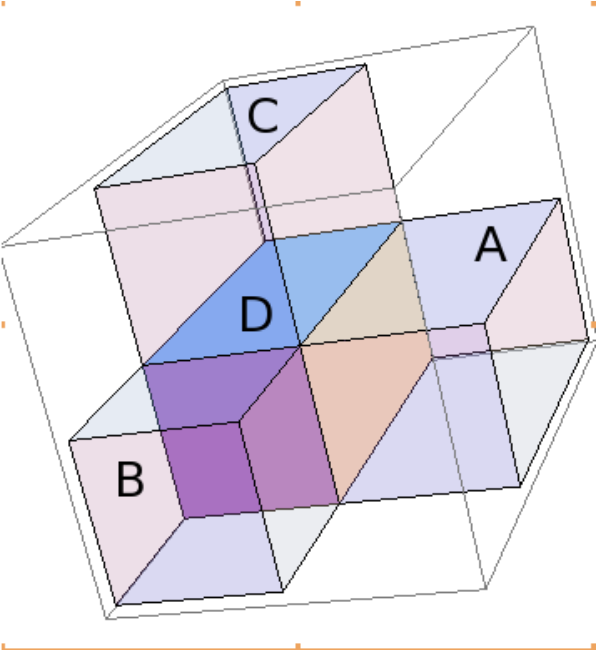
Refer to caption
Figure 2: Constraints on the dimensions of the tensors implied by the ternary product definition.

We note that matrix product is a special instance of a tensor product and we shall discuss subsequently products of nn-tensor where nn is positive integer greater or equal to 22. Furthermore the proposed definition of the tensor multiplication suggests a generalization of the binary vector outer product operator to a ternary operator of slices. The ternary outer product is defined such that given tensors 𝑨\boldsymbol{A} of dimensions (m×1×p)(m\times 1\times p), 𝑩\boldsymbol{B} of dimensions (m×n×1)(m\times n\times 1), and 𝑪\boldsymbol{C} of dimensions (1×n×p)(1\times n\times p), their ternary outer product 𝑫\boldsymbol{D}, noted 𝑫=⊗(𝑨,𝑩,𝑪)\boldsymbol{D}=\otimes(\boldsymbol{A},\boldsymbol{B},\boldsymbol{C}), is an (m×n×p)(m\times n\times p) tensor defined by :

di,j,k=ai,1,k⋅bi,j,1⋅c1,j,k.d_{i,j,k}=a_{i,1,k}\cdot b_{i,j,1}\cdot c_{1,j,k}. (26)

Note that 𝑨\boldsymbol{A}, 𝑩,\boldsymbol{B}, and 𝑪\boldsymbol{C} here are slices arising from oriented matrices. The above definition generalizes the binary vector outer product operation to a ternary matrix outer product operation defined by

𝑫=⊗(𝒂∙,1,∙,𝒃∙,∙,1,𝒄1,∙,∙):=di,j,k=ai,1,k⋅bi,j,1⋅c1,j,k.\boldsymbol{D}=\otimes\left(\boldsymbol{a}_{\centerdot,1,\centerdot},\>\boldsymbol{b}_{\centerdot,\centerdot,1},\;\boldsymbol{c}_{1,\centerdot,\centerdot}\right)\;:=d_{i,j,k}=a_{i,1,k}\cdot b_{i,j,1}\cdot c_{1,j,k}. (27)

Similarly to matrix multiplication, where the operation of multiplying appropriate sized matrices can be viewed as a summation of outer product of vectors, the product of appropriate sized triplet of tensors in Eq  25 can be viewed as a summation of ternary outer product of slices

∘(𝑨,𝑩,𝑪)≡∑1≤t≤l⊗(𝒂∙,t,∙,𝒃∙,∙,t,𝒄t,∙,∙).\circ\left(\boldsymbol{A},\boldsymbol{B},\boldsymbol{C}\right)\equiv\sum_{1\leq t\leq l}\otimes\left(\boldsymbol{a}_{\centerdot,t,\centerdot},\>\boldsymbol{b}_{\centerdot,\centerdot,t},\;\boldsymbol{c}_{t,\centerdot,\centerdot}\right). (28)


Ternary dot product with a background tensor: The ternary dot product above can be further generalized by introducing the notion of a background tensor as follows for 𝒂1,∙,1=(a1,i,1){1≤i≤l}\boldsymbol{a}_{1,\centerdot,1}=\left(a_{1,i,1}\right)_{\left\{1\leq i\leq l\right\}}, 𝒃1,1,∙=(b1,1,j){1≤j≤l}\boldsymbol{b}_{1,1,\centerdot}=\left(b_{1,1,j}\right)_{\left\{1\leq j\leq l\right\}} and 𝒄∙,1,1=(ck,1,1){1≤k≤l}\boldsymbol{c}_{\centerdot,1,1}=\left(c_{k,1,1}\right)_{\left\{1\leq k\leq l\right\}}

⟨𝒂1,∙,1,𝒃1,1,∙,𝒄∙,1,1⟩𝑻:=∑1≤i≤l(∑1≤j≤l(∑1≤k≤la1,i,1⋅b1,1,j𝔠31⋅ck,1,1𝔠32⋅ti,j,k))\left\langle\boldsymbol{a}_{1,\centerdot,1},\boldsymbol{b}_{1,1,\centerdot},\boldsymbol{c}_{\centerdot,1,1}\right\rangle_{\boldsymbol{T}}\;:=\sum_{1\leq i\leq l}\left(\sum_{1\leq j\leq l}\left(\sum_{1\leq k\leq l}a_{1,i,1}\cdot b_{1,1,j}^{\mathfrak{c}_{3}^{1}}\cdot c_{k,1,1}^{\mathfrak{c}_{3}^{2}}\cdot t_{i,j,k}\right)\right) (29)

the preceding will be referred to as the triplet dot product operator with background tensor 𝑻\boldsymbol{T}. Background tensors plays a role analogous to that of the metric tensor. The triplet dot product with non trivial background tensor corresponds to a pure trilinear form. Furthermore the outer product of 22-tensors can be generalized using the notion of background tensors to produce a 33-tensor 𝑫\boldsymbol{D} which result from a product of three 22-tensors namely 𝒂∙,∙,1=(am,i,1)m,i\boldsymbol{a}_{\centerdot,\centerdot,1}=\left(a_{m,i,1}\right)_{m,i}, 𝒃1,∙,∙=(b1,n,j)n,j\boldsymbol{b}_{1,\centerdot,\centerdot}=\left(b_{1,n,j}\right)_{n,j} and 𝒄∙,1,∙=(ck,1,p)k,p\boldsymbol{c}_{\centerdot,1,\centerdot}=\left(c_{k,1,p}\right)_{k,p} as follows,

dm,n,p=∑1≤i≤l(∑1≤j≤l(∑1≤k≤lam,i,1⋅b1,n,j⋅ck,1,p⋅ti,j,k)).d_{m,n,p}=\sum_{1\leq i\leq l}\left(\sum_{1\leq j\leq l}\left(\sum_{1\leq k\leq l}a_{m,i,1}\cdot b_{1,n,j}\cdot c_{k,1,p}\cdot t_{i,j,k}\right)\right). (30)

The preceding product expression is the one most commonly used as a basis for tensor algebra in the literature as discussed in [6, 34, 7, 19].
We may note that the original definition of the dot product for a triplets of vectors corresponds to a setting where the background tensor is the Kronecker delta 𝚫=(δi,j,k)\boldsymbol{\Delta}=\left(\delta_{i,j,k}\right) that is 𝑻=𝚫\boldsymbol{T}=\boldsymbol{\Delta} where 𝚫\boldsymbol{\Delta} denotes hereafter the Kronecker tensor and can be expressed in terms of the Kronecker 22-tensors as follows

δi,j,k=δi,j⋅δj,k⋅δk,i\delta_{i,j,k}=\delta_{i,j}\cdot\delta_{j,k}\cdot\delta_{k,i} (31)

equivalently 𝚫=(δi,j,k)\boldsymbol{\Delta}=\left(\delta_{i,j,k}\right) can be expressed in terms of the canonical basis {𝒆i: 1≤i≤l}\left\{\boldsymbol{e}_{i}:\;1\leq i\leq l\right\} in ll-dimensional euclidean space described by:

𝚫=∑1≤k≤l(𝒆k⊗𝒆k⊗𝒆k),\boldsymbol{\Delta}=\sum_{1\leq k\leq l}\left(\boldsymbol{e}_{k}\otimes\boldsymbol{e}_{k}\otimes\boldsymbol{e}_{k}\right), (32)
Refer to caption
Figure 3: Kronecker (2×2×2)\left(2\times 2\times 2\right) tensor.

hence

⟨𝒘,𝒙,𝒚⟩≡⟨𝒘,𝒙,𝒚⟩𝚫.\langle\boldsymbol{w},\,\boldsymbol{x},\,\boldsymbol{y}\rangle\equiv\langle\boldsymbol{w},\,\boldsymbol{x},\,\boldsymbol{y}\rangle_{\boldsymbol{\Delta}}. (33)

3.1.1 Special Tensors and Special Operations

In general it follows from the algebra described in the previous section for 33-tensors that:

∘(∘(𝑨,𝑩,𝑪),𝑫,𝑬)≠∘(𝑨,∘(𝑩,𝑪,𝑫),𝑬)≠∘(𝑨,𝑩,∘(𝑪,𝑫,𝑬))\circ\left(\circ\left(\boldsymbol{A},\boldsymbol{B},\boldsymbol{C}\right),\boldsymbol{D},\boldsymbol{E}\right)\neq\circ\left(\boldsymbol{A},\circ\left(\boldsymbol{B},\boldsymbol{C},\boldsymbol{D}\right),\boldsymbol{E}\right)\neq\circ\left(\boldsymbol{A},\boldsymbol{B},\circ\left(\boldsymbol{C},\boldsymbol{D},\boldsymbol{E}\right)\right) (34)

In some sense the preceding illustrates the fact that the product operator is non associative over the set of tensors. However tensor product is weakly distributive over tensor addition that is to say

∘([𝑨+𝑩],𝑪,𝑫))=∘(𝑨,𝑪,𝑫)+∘(𝑩,𝑪,𝑫),\circ\left(\left[\boldsymbol{A}+\boldsymbol{B}\right],\,\boldsymbol{C},\,\boldsymbol{D}\right))=\circ\left(\boldsymbol{A},\boldsymbol{C},\boldsymbol{D}\right)+\circ\left(\boldsymbol{B},\boldsymbol{C},\boldsymbol{D}\right), (35)

however in general

∘(𝑨,∘(𝑩,𝑪,𝑫),𝑬)+∘(𝑨,∘(𝑭,𝑮,𝑯),𝑬)≠∘(𝑨,(∘(𝑩,𝑪,𝑫)+∘(𝑭,𝑮,𝑯)),𝑬).\circ\left(\boldsymbol{A},\circ\left(\boldsymbol{B},\boldsymbol{C},\boldsymbol{D}\right),\boldsymbol{E}\right)+\circ\left(\boldsymbol{A},\circ\left(\boldsymbol{F},\boldsymbol{G},\boldsymbol{H}\right),\boldsymbol{E}\right)\neq\circ\left(\boldsymbol{A},\,\left(\circ\left(\boldsymbol{B},\boldsymbol{C},\boldsymbol{D}\right)+\circ\left(\boldsymbol{F},\boldsymbol{G},\boldsymbol{H}\right)\right)\,,\boldsymbol{E}\right). (36)


Transpose of a tensor: Given a tensor 𝑨=(au,v,w)\boldsymbol{A}=\left(a_{u,v,w}\right) we define it’s transpose 𝑨T\boldsymbol{A}^{T} and it’s double transpose 𝑨T2\boldsymbol{A}^{T^{2}}as follows:

𝑨T=(av,w,u)\boldsymbol{A}^{T}=\left(a_{v,w,u}\right) (37)
𝑨T2≡(𝑨T)T=(aw,u,v).\boldsymbol{A}^{T^{2}}\equiv\left(\boldsymbol{A}^{T}\right)^{T}=\left(a_{w,u,v}\right). (38)

It immediately follows from the definition of the transpose that for any tensor 𝑨\boldsymbol{A}, 𝑨T3=𝑨.\boldsymbol{A}^{T^{3}}=\boldsymbol{A}. Incidentally the transpose operator corresponds to a cyclic permutation of the indices of the entries of 𝑨\boldsymbol{A}. Therefore we can defined a inverse transpose 𝑨T−1=𝑨T2\boldsymbol{A}^{T^{-1}}=\boldsymbol{A}^{T^{2}}, generally we have

𝑨Tq=(𝑨Tq−1)T,\boldsymbol{A}^{T^{q}}=\left(\boldsymbol{A}^{T^{q-1}}\right)^{T}, (39)

furthermore, a tensor 𝑨\boldsymbol{A} is said to be symmetrical if :

𝑨=𝑨T=𝑨T2.\boldsymbol{A}=\boldsymbol{A}^{T}=\boldsymbol{A}^{T^{2}}. (40)

As a result for a given arbitrary 33-tensor 𝑨\boldsymbol{A}, the products 𝑩=∘(𝑨,𝑨T2,𝑨T)\boldsymbol{B}=\circ\left(\boldsymbol{A},\boldsymbol{A}^{T^{2}},\boldsymbol{A}^{T}\right), 𝑪=∘(𝑨T,𝑨,𝑨T2)\boldsymbol{C}=\circ\left(\boldsymbol{A}^{T},\boldsymbol{A},\boldsymbol{A}^{T^{2}}\right) and 𝑫=∘(𝑨T2,𝑨T,𝑨)\boldsymbol{D}=\circ\left(\boldsymbol{A}^{T^{2}},\boldsymbol{A}^{T},\boldsymbol{A}\right) all result in symmetric tensors. It also follows from the definitions of the transpose operation and the definition of ternary product operation that:

[∘(𝑨,𝑩,𝑪)]T=∘(𝑩T,𝑪T,𝑨T)\left[\circ\left(\boldsymbol{A},\boldsymbol{B},\boldsymbol{C}\right)\right]^{T}=\circ\left(\boldsymbol{B}^{T},\boldsymbol{C}^{T},\boldsymbol{A}^{T}\right) (41)

and

[∘(𝑨,𝑩,𝑪)]T2=[∘(𝑩T,𝑪T,𝑨T)]T=∘(𝑪T2,𝑨T2,𝑩T2).\left[\circ\left(\boldsymbol{A},\boldsymbol{B},\boldsymbol{C}\right)\right]^{T^{2}}=\left[\circ\left(\boldsymbol{B}^{T},\boldsymbol{C}^{T},\boldsymbol{A}^{T}\right)\right]^{T}=\circ\left(\boldsymbol{C}^{T^{2}},\boldsymbol{A}^{T^{2}},\boldsymbol{B}^{T^{2}}\right). (42)

Adjoint operator: For 𝑨∈ℂm×n×p\boldsymbol{A}\in\mathbb{C}^{m\times n\times p} we introduce the analog of the adjoint operator for 33-tensors in two steps. The first step consists in writing all the entries of 𝑨\boldsymbol{A} in their complex polar form.

𝑨=(au,v,w=ru,v,w⋅exp{i⋅θu,v,w})(1≤u≤m; 1≤v≤n; 1≤w≤p).\boldsymbol{A}=\left(a_{u,v,w}=r_{u,v,w}\cdot\exp\left\{i\cdot\theta_{u,v,w}\right\}\right)\;\left(1\leq u\leq m;\,1\leq v\leq n;\,1\leq w\leq p\right). (43)

The final step expresses the adjoint of the tensor 𝑨\boldsymbol{A} noted 𝑨†\boldsymbol{A}^{\dagger} as follows

{𝑨†≡(𝑨𝔠31)T:=(rv,w,u⋅exp⁡{i​exp⁡{i​2​π3}⋅θv,w,u})𝑨†2≡(𝑨𝔠32)T2:=(rw,u,v⋅exp{iexp{i4​π3}⋅θw,u,v})𝑨†3≡(𝑨𝔠33)T3:=(au,v,w=ru,v,w⋅exp{i⋅θu,v,w}).\begin{cases}\begin{array}[]{c}\boldsymbol{A}^{\dagger}\equiv\left(\boldsymbol{A}^{\mathfrak{c}_{3}^{1}}\right)^{T}\>:=\left(r_{v,w,u}\cdot\exp\left\{i\,\exp\left\{i\>\frac{2\pi}{3}\right\}\cdot\theta_{v,w,u}\right\}\right)\\ \boldsymbol{A}^{\dagger^{2}}\equiv\left(\boldsymbol{A}^{\mathfrak{c}_{3}^{2}}\right)^{T^{2}}\>:=\left(r_{w,u,v}\cdot\exp\left\{i\,\exp\left\{i\>\frac{4\pi}{3}\right\}\cdot\theta_{w,u,v}\right\}\right)\\ \boldsymbol{A}^{\dagger^{3}}\equiv\left(\boldsymbol{A}^{\mathfrak{c}_{3}^{3}}\right)^{T^{3}}\>:=\left(a_{u,v,w}=r_{u,v,w}\cdot\exp\left\{i\cdot\theta_{u,v,w}\right\}\right)\end{array}&.\end{cases} (44)

The adjoint operator introduced here allows us to generalize the notion of Hermitian matrices or self adjoint matrices to tensors. A tensor is Hermitian if the following identity holds

𝑨†=𝑨.\boldsymbol{A}^{\dagger}=\boldsymbol{A}. (45)

Incidentally the products ∘(𝑨,𝑨†2,𝑨†)\circ\left(\boldsymbol{A},\boldsymbol{A}^{\dagger^{2}},\boldsymbol{A}^{\dagger}\right), ∘(𝑨†,𝑨,𝑨†2)\circ\left(\boldsymbol{A}^{\dagger},\boldsymbol{A},\boldsymbol{A}^{\dagger^{2}}\right) and ∘(𝑨†2,𝑨†,𝑨)\circ\left(\boldsymbol{A}^{\dagger^{2}},\boldsymbol{A}^{\dagger},\boldsymbol{A}\right) result in self adjoint tensors or Hermitian tensors.
Identity Tensor: Let 𝟏(m×n×p)\boldsymbol{1}_{(m\times n\times p)} denotes the tensor having all it’s entries equal to one and of dimensions (m×n×p)(m\times n\times p). Recalling that 𝚫=(δi,j,k)\boldsymbol{\Delta}=\left(\delta_{i,j,k}\right) denotes the Kronecker 3-tensor, we define the identity tensors 𝑰\boldsymbol{I} to be :

𝑰=∘(𝟏(l×l×l),𝟏(l×l×l),𝚫)=∘(𝟏(l×l×l),𝟏(l×l×l),(∑1≤k≤l𝒆k⊗𝒆k⊗𝒆k))\boldsymbol{I}=\circ\left(\boldsymbol{1}_{(l\times l\times l)},\boldsymbol{1}_{(l\times l\times l)},\boldsymbol{\Delta}\right)=\circ\left(\boldsymbol{1}_{(l\times l\times l)},\boldsymbol{1}_{(l\times l\times l)},\left(\sum_{1\leq k\leq l}\boldsymbol{e}_{k}\otimes\boldsymbol{e}_{k}\otimes\boldsymbol{e}_{k}\right)\right) (46)
𝑰≡(im,n,p=(∑1≤k≤lδk,n,p)=δn,p)\boldsymbol{I}\equiv\left(i_{m,n,p}=\left(\sum_{1\leq k\leq l}\delta_{k,n,p}\right)=\delta_{n,p}\right) (47)

Furthermore we have :

𝑰T=∘(𝟏(l×l×l),𝚫,𝟏(l×l×l))=∘(𝟏(l×l×l),(∑1≤k≤l𝒆k⊗𝒆k⊗𝒆k),𝟏(l×l×l))\boldsymbol{I}^{T}=\circ\left(\boldsymbol{1}_{(l\times l\times l)},\boldsymbol{\Delta},\boldsymbol{1}_{(l\times l\times l)}\right)=\circ\left(\boldsymbol{1}_{(l\times l\times l)},\left(\sum_{1\leq k\leq l}\boldsymbol{e}_{k}\otimes\boldsymbol{e}_{k}\otimes\boldsymbol{e}_{k}\right),\boldsymbol{1}_{(l\times l\times l)}\right) (48)
𝑰T≡((𝑰T)m,n,p=(∑1≤k≤lδm,n,k)=δm,n)\boldsymbol{I}^{T}\equiv\left(\left(\boldsymbol{I}^{T}\right)_{m,n,p}=\left(\sum_{1\leq k\leq l}\delta_{m,n,k}\right)=\delta_{m,n}\right) (49)
𝑰T2=∘(𝚫,𝟏(l×l×l),𝟏(l×l×l))=∘((∑1≤k≤l𝒆k⊗𝒆k⊗𝒆k),𝟏(l×l×l),𝟏(l×l×l))\boldsymbol{I}^{T^{2}}=\circ\left(\boldsymbol{\Delta},\boldsymbol{1}_{(l\times l\times l)},\boldsymbol{1}_{(l\times l\times l)}\right)=\circ\left(\left(\sum_{1\leq k\leq l}\boldsymbol{e}_{k}\otimes\boldsymbol{e}_{k}\otimes\boldsymbol{e}_{k}\right),\boldsymbol{1}_{(l\times l\times l)},\boldsymbol{1}_{(l\times l\times l)}\right) (50)
𝑰T2≡((𝑰T2)m,n,p=(∑1≤k≤lδm,k,p)=δm,p)\boldsymbol{I}^{T^{2}}\equiv\left(\left(\boldsymbol{I}^{T^{2}}\right)_{m,n,p}=\left(\sum_{1\leq k\leq l}\delta_{m,k,p}\right)=\delta_{m,p}\right) (51)

for all positive integer l≥2l\geq 2 . The identity tensor plays a role quite analogous to the role of the identity matrix since ∀𝑨∈ℂl×l×l\forall\,\boldsymbol{A}\in\mathbb{C}^{l\times l\times l} we have

∘(𝑰,𝑨,𝑰T2)=𝑨.\circ\left(\boldsymbol{I},\boldsymbol{A},\boldsymbol{I}^{T^{2}}\right)=\boldsymbol{A}. (52)

Proposition 1: ∀𝐀∘(𝐗,𝐀,𝐗T2)=𝐀and𝐗=(xm,n,p≥0)⇔𝐗=𝐈\forall\boldsymbol{A}\quad\circ\left(\boldsymbol{X},\boldsymbol{A},\boldsymbol{X}^{T^{2}}\right)=\boldsymbol{A}\quad and\quad\boldsymbol{X=}\left(x_{m,n,p}\geq 0\right)\Leftrightarrow\boldsymbol{X}=\boldsymbol{I}
We prove the preceding assertion in two steps, the first step consists of showing that the 𝑰\boldsymbol{I} is indeed a solution to the equation

∀𝑨∘(𝑿,𝑨,𝑿T2)=𝑨\forall\boldsymbol{A}\quad\circ\left(\boldsymbol{X},\boldsymbol{A},\boldsymbol{X}^{T^{2}}\right)=\boldsymbol{A} (53)

Let 𝑹\boldsymbol{R} be the result of the product

𝑹=(rm,n,p)=∘(𝑰,𝑨,𝑰T2)\boldsymbol{R}=\left(r_{m,n,p}\right)=\circ\left(\boldsymbol{I},\boldsymbol{A},\boldsymbol{I}^{T^{2}}\right) (54)
rm,n,p=(∑1≤k≤lim,k,p⋅am,n,k⋅(𝑰T2)k,n,p)=(∑1≤k≤lδk,p⋅am,n,k⋅δk,p)r_{m,n,p}=\left(\sum_{1\leq k\leq l}i_{m,k,p}\cdot a_{m,n,k}\cdot\left(\boldsymbol{I}^{T^{2}}\right)_{k,n,p}\right)=\left(\sum_{1\leq k\leq l}\delta_{k,p}\cdot a_{m,n,k}\cdot\delta_{k,p}\right) (55)
rm,n,p=(∑1≤k≤l(δk,p)2⋅am,n,k)r_{m,n,p}=\left(\sum_{1\leq k\leq l}\left(\delta_{k,p}\right)^{2}\cdot a_{m,n,k}\right) (56)

we note that

rm,n,k={am,n,k​i​f​k=p0​o​t​h​e​r​w​i​s​er_{m,n,k}=\begin{cases}\begin{array}[]{c}a_{m,n,k}\;if\>k=p\\ 0\;otherwise\end{array}\end{cases} (57)

hence

𝑨=∘(𝑰,𝑨,𝑰T2).\boldsymbol{A}=\circ\left(\boldsymbol{I},\boldsymbol{A},\boldsymbol{I}^{T^{2}}\right). (58)

The last step consists in proving by contradiction that 𝑰\boldsymbol{I} is the unique solution with positive entries to the equation

∀𝑨∘(𝑿,𝑨,𝑿T2)=𝑨\forall\boldsymbol{A}\quad\circ\left(\boldsymbol{X},\boldsymbol{A},\boldsymbol{X}^{T^{2}}\right)=\boldsymbol{A} (59)

Suppose there were some other solution 𝑱\boldsymbol{J} with positive entry to the above equation, this would imply that

∘(𝑰,𝑨,𝑰T2)−∘(𝑱,𝑨,𝑱T2)=0\circ\left(\boldsymbol{I},\boldsymbol{A},\boldsymbol{I}^{T^{2}}\right)-\quad\circ\left(\boldsymbol{J},\boldsymbol{A},\boldsymbol{J}^{T^{2}}\right)=0 (60)
⇒(∑1≤k≤lim,k,p⋅am,n,k⋅(𝑰T2)k,n,p)−(∑1≤k≤ljm,k,p⋅am,n,k⋅(𝑱T2)k,n,p)\Rightarrow\left(\sum_{1\leq k\leq l}i_{m,k,p}\cdot a_{m,n,k}\cdot\left(\boldsymbol{I}^{T^{2}}\right)_{k,n,p}\right)-\left(\sum_{1\leq k\leq l}j_{m,k,p}\cdot a_{m,n,k}\cdot\left(\boldsymbol{J}^{T^{2}}\right)_{k,n,p}\right) (61)
0=∑1≤k≤lam,n,k⋅[(im,k,p⋅(𝑰T2)k,n,p)−(jm,k,p⋅(𝑱T2)k,n,p)]0=\sum_{1\leq k\leq l}a_{m,n,k}\cdot\left[\left(i_{m,k,p}\cdot\left(\boldsymbol{I}^{T^{2}}\right)_{k,n,p}\right)-\left(j_{m,k,p}\cdot\left(\boldsymbol{J}^{T^{2}}\right)_{k,n,p}\right)\right] (62)

Since this expression must be true for any choice of the values of am,n,ka_{m,n,k} we deduce that it must be the case that

(δk,p)2−(jm,k,p⋅(𝑱T2)k,n,p)=0\left(\delta_{k,p}\right)^{2}-\left(j_{m,k,p}\cdot\left(\boldsymbol{J}^{T^{2}}\right)_{k,n,p}\right)=0 (63)
⇒(jm,k,p⋅(𝑱T2)k,n,p)=δk,p\Rightarrow\left(j_{m,k,p}\cdot\left(\boldsymbol{J}^{T^{2}}\right)_{k,n,p}\right)=\delta_{k,p} (64)
jm,k,p=±δk,pj_{m,k,p}=\pm\delta_{k,p} (65)

the requirement that

jm,k,p≥0⇒jm,k,p=δk,pj_{m,k,p}\geq 0\Rightarrow j_{m,k,p}=\delta_{k,p} (66)

which results in the sought after contradiction □\square.

Refer to caption
Refer to caption
Refer to caption
Figure 4: Tensor 𝑰\boldsymbol{I},𝑰T\boldsymbol{I}^{T}and 𝑰T2\boldsymbol{I}^{T^{2}}

Inverse: By analogy to matrix inverse 𝑨−1\boldsymbol{A}^{-1} we recall that for a matrix 𝑨\boldsymbol{A}, 𝑨−1\boldsymbol{A}^{-1} is its inverse if (𝑴​𝑨)​𝑨−1=𝑴\left(\boldsymbol{M}\boldsymbol{A}\right)\boldsymbol{A}^{-1}=\boldsymbol{M}, for any non zero matrix 𝑴\boldsymbol{M}. We introduce here the notion of inverse pairs for tensors. The ordered pair (𝑨1,𝑨2)\left(\boldsymbol{A}_{1},\boldsymbol{A}_{2}\right) and (𝑩1,𝑩2)\left(\boldsymbol{B}_{1},\boldsymbol{B}_{2}\right) are related by inverse relationship if for any non zero 33-tensor 𝑴\boldsymbol{M} with appropriated dimensions the following identity holds

𝑴=∘(𝑩1∘(𝑨1,𝑴,𝑨2),𝑩2).\boldsymbol{M}=\circ\left(\boldsymbol{B}_{1}\circ\left(\boldsymbol{A}_{1},\boldsymbol{M},\boldsymbol{A}_{2}\right),\boldsymbol{B}_{2}\right). (67)


Permutation tensors: Incidentally one may also discuss the notion of permutation tensors associated with any element σ\sigma of the permutation group SnS_{n}.

∀σ∈Sn𝑷σ≡∘(𝟏(n×n×n),𝟏(n×n×n),(∑1≤k≤l𝒆k⊗𝒆k⊗𝒆σ⁡(k)))\forall\;\sigma\in S_{n}\;\boldsymbol{P}_{\sigma}\equiv\circ\left(\boldsymbol{1}_{(n\times n\times n)},\boldsymbol{1}_{(n\times n\times n)},\left(\sum_{1\leq k\leq l}\boldsymbol{e}_{k}\otimes\boldsymbol{e}_{k}\otimes\boldsymbol{e}_{\sigma\left(k\right)}\right)\right) (68)
=∑1≤k≤l∘(𝟏(n×n×n),𝟏(n×n×n),(𝒆k⊗𝒆k⊗𝒆σ⁡(k)))=\sum_{1\leq k\leq l}\circ\left(\boldsymbol{1}_{(n\times n\times n)},\boldsymbol{1}_{(n\times n\times n)},\left(\boldsymbol{e}_{k}\otimes\boldsymbol{e}_{k}\otimes\boldsymbol{e}_{\sigma\left(k\right)}\right)\right) (69)

The 33-tensor 𝑷σ\boldsymbol{P}_{\sigma} perform the permutation σ\sigma on the depth slices of a 33-tensor 𝑨\boldsymbol{A} through the product ∘(𝑷σ,𝑨,𝑷σT2)\circ\left(\boldsymbol{P}_{\sigma},\,\boldsymbol{A},\,\boldsymbol{P}_{\sigma}^{T^{2}}\right) , consequently the products ∘(𝑷σT,𝑷σT2,𝑨)\circ\left(\boldsymbol{P}_{\sigma}^{T},\,\boldsymbol{P}_{\sigma}^{T^{2}},\boldsymbol{A}\right) and ∘(𝑨,𝑷σ,𝑷σT)\circ\left(\boldsymbol{A}\,,\boldsymbol{P}_{\sigma},\,\boldsymbol{P}_{\sigma}^{T}\right) perform the same permutation respectively on the row slices and the column slices of 𝑨\boldsymbol{A}.

Proposition 2: Any permutation of the depth slices of 𝑨\boldsymbol{A} can be obtained by finite sequence of product of transposition, and the sequence is of the form

∘(𝑷σn,⋯,∘(𝑷σk,⋯,∘(𝑷σ1,𝑨,(𝑷σ1)T2)⋯,(𝑷σk)T2),⋯,(𝑷σn)T2).\circ\left(\boldsymbol{P}\sigma_{n},\cdots,\circ\left(\boldsymbol{P}\sigma_{k},\cdots,\circ\left(\boldsymbol{P}\sigma_{1},\boldsymbol{A},\left(\boldsymbol{P}\sigma_{1}\right)^{T^{2}}\right)\cdots,\left(\boldsymbol{P}\sigma_{k}\right)^{T^{2}}\right),\cdots,\left(\boldsymbol{P}\sigma_{n}\right)^{T^{2}}\right). (70)

The preceding is easily verified using the definition above and the permutation decomposition theorem [8]. Furthermore permutation tensors suggest a generalization of bi-stochastic matrices to bi-stochastic tensors through the Birkhoff-Von Neumann bi-stochastic matrix theorem.

3.1.2 Orthogonality and scaling tensors

From linear algebra we know that permutation matrices belong to both the set of bi-stochastic matrices and to the set of orthogonal matrices. We described above a approach for defining bi-stochastic 33-tensors, we shall address in this section the notion of orthogonality for 33-tensors. We recall from linear algebra that a matrix 𝑸\boldsymbol{Q} is said to be orthogonal if

𝑸†⋅𝑸=𝑸⋅𝑸†=𝚫.\boldsymbol{Q}^{\dagger}\cdot\boldsymbol{Q}=\boldsymbol{Q}\cdot\boldsymbol{Q}^{\dagger}=\boldsymbol{\Delta}. (71)

When we consider the corresponding equation for 3-tensors two distinct interpretations arise. The first interpretation related to orthonormal basis induced by the row or column vectors of the orthogonal matrix 𝑸\boldsymbol{Q} that is :

⟨𝒒∙,m,𝒒∙,n⟩≡⟨𝒒m,𝒒n⟩=(∑1≤k≤lqk,m⋅qk,n𝔠21)=δm,n\left\langle\boldsymbol{q}_{\centerdot,m},\boldsymbol{q}_{\centerdot,n}\right\rangle\equiv\left\langle\boldsymbol{q}_{m},\boldsymbol{q}_{n}\right\rangle=\left(\sum_{1\leq k\leq l}q_{k,m}\cdot q_{k,n}^{\mathfrak{c}_{2}^{1}}\right)=\delta_{m,n} (72)

The corresponding equation for a 33-tensor 𝑸=(qm,n,p)\boldsymbol{Q}=\left(q_{m,n,p}\right) of dimensions (l×l×l)\left(l\times l\times l\right) is given by:

𝚫=∘(𝑸,𝑸†2,𝑸†)\boldsymbol{\Delta}=\circ\left(\boldsymbol{Q},\boldsymbol{Q}^{\dagger^{2}},\boldsymbol{Q}^{\dagger}\right) (73)

or explicitly we can write:

⟨𝒒m,∙,p,𝒒n,∙,m,𝒒p,∙,n⟩=(∑1≤k≤lqm,k,p⋅qn,k,m𝔠32⋅qp,k,n𝔠31)=δm,n,p.\left\langle\boldsymbol{q}_{m,\centerdot,p},\boldsymbol{q}_{n,\centerdot,m},\boldsymbol{q}_{p,\centerdot,n}\right\rangle=\left(\sum_{1\leq k\leq l}q_{m,k,p}\cdot q_{n,k,m}^{\mathfrak{c}_{3}^{2}}\cdot q_{p,k,n}^{\mathfrak{c}_{3}^{1}}\right)=\delta_{m,n,p}. (74)

The second interpretation arises from the Kronecker invariance equation expressed by:

𝚫=𝑸†​𝚫​𝑸=(𝑸†​𝚫​𝑸)†.\boldsymbol{\Delta}=\boldsymbol{Q}^{\dagger}\boldsymbol{\Delta}\boldsymbol{Q}=\left(\boldsymbol{Q}^{\dagger}\boldsymbol{\Delta}\boldsymbol{Q}\right)^{\dagger}. (75)

The corresponding Kronecker invariance equation for 33-tensor is given by :

𝚫=∘(∘(𝑸,∘(𝑸†,𝑸†2,𝚫),𝑸†2),𝑸,𝑸†)\boldsymbol{\Delta}=\circ\left(\circ\left(\boldsymbol{Q},\circ\left(\boldsymbol{Q}^{\dagger},\boldsymbol{Q}^{\dagger^{2}},\boldsymbol{\Delta}\right),\boldsymbol{Q}^{\dagger^{2}}\right),\boldsymbol{Q},\boldsymbol{Q}^{\dagger}\right)
=[∘(∘(𝑸,∘(𝑸†,𝑸†2,𝚫),𝑸†2),𝑸,𝑸†)]†=[∘(∘(𝑸,∘(𝑸†,𝑸†2,𝚫),𝑸†2),𝑸,𝑸†)]†2.=\left[\circ\left(\circ\left(\boldsymbol{Q},\circ\left(\boldsymbol{Q}^{\dagger},\boldsymbol{Q}^{\dagger^{2}},\boldsymbol{\Delta}\right),\boldsymbol{Q}^{\dagger^{2}}\right),\boldsymbol{Q},\boldsymbol{Q}^{\dagger}\right)\right]^{\dagger}=\left[\circ\left(\circ\left(\boldsymbol{Q},\circ\left(\boldsymbol{Q}^{\dagger},\boldsymbol{Q}^{\dagger^{2}},\boldsymbol{\Delta}\right),\boldsymbol{Q}^{\dagger^{2}}\right),\boldsymbol{Q},\boldsymbol{Q}^{\dagger}\right)\right]^{\dagger^{2}}. (76)

While Kronecker invariance properly expresses a generalization of the conjugation operation and the 33-uniform hypergraph isomorphism equation it does not follow from the first interpretation of orthogonality, that is to say

𝚫=∘(𝑸,𝑸†2,𝑸†)⇏∘(∘(𝑸,∘(𝑸†,𝑸†2,𝚫),𝑸†2),𝑸,𝑸†)=𝚫.\boldsymbol{\Delta}=\circ\left(\boldsymbol{Q},\boldsymbol{Q}^{\dagger^{2}},\boldsymbol{Q}^{\dagger}\right)\nRightarrow\circ\left(\circ\left(\boldsymbol{Q},\circ\left(\boldsymbol{Q}^{\dagger},\boldsymbol{Q}^{\dagger^{2}},\boldsymbol{\Delta}\right),\boldsymbol{Q}^{\dagger^{2}}\right),\boldsymbol{Q},\boldsymbol{Q}^{\dagger}\right)=\boldsymbol{\Delta}. (77)

We now discuss Scaling tensors. The scaling tensor play a role analogous to diagonal matrices in the fact that tensor multiplication with scalling tensor results in a tensor whose vectors are scalled. First we observe that the identity pairs of tensors should corespond to special scaling tensors. The general family of diagonal tensors are expressed by pairs of tensors 𝑩=(bm,n,p)\boldsymbol{B}=\left(b_{m,n,p}\right) , 𝑪=(cm,n,p)\boldsymbol{C}=\left(c_{m,n,p}\right) such that

𝑩≡(bm,n,p=δn,p⋅wp,m)\boldsymbol{B}\equiv\left(b_{m,n,p}=\delta_{n,p}\cdot w_{p,m}\right) (78)
𝑪≡(cm,n,p=δm,n⋅wm,p)\boldsymbol{C}\equiv\left(c_{m,n,p}=\delta_{m,n}\cdot w_{m,p}\right) (79)

The product 𝑫=∘(𝑨,𝑩,𝑪)\boldsymbol{D}=\circ\left(\boldsymbol{A},\boldsymbol{B},\boldsymbol{C}\right) yields

dm,n,p=∑1≤k≤lam,k,p⋅(δn,k⋅wm,k)⋅(δk,n⋅wk,p)d_{m,n,p}=\sum_{1\leq k\leq l}a_{m,k,p}\cdot\left(\delta_{n,k}\cdot w_{m,k}\right)\cdot\left(\delta_{k,n}\cdot w_{k,p}\right) (80)
⇒dm,n,p=wm,n⋅am,n,p⋅wn,p\Rightarrow d_{m,n,p}=w_{m,n}\cdot a_{m,n,p}\cdot w_{n,p} (81)

The expression above illustrates the fact that wm,nw_{m,n} and wn,pw_{n,p} scale the entry am,n,pa_{m,n,p} of the tensor 𝑨\boldsymbol{A}, or equivalently one may view the expression above as describing the non-uniform scaling of the following vector (am,n,p)1≤n≤l\left(a_{m,n,p}\right)_{1\leq n\leq l}. The vector scaling transform is expressed by

(am,n,p)1≤n≤l→(wm,n⋅am,n,p⋅wn,p)1≤n≤l\left(a_{m,n,p}\right)_{1\leq n\leq l}\rightarrow\left(w_{m,n}\cdot a_{m,n,p}\cdot w_{n,p}\right)_{1\leq n\leq l} (82)

Furthermore the scaling factors for a given vector may be viewed as coming from the same vector of the scaling matrix 𝑾=(wm,n)\boldsymbol{W}=\left(w_{m,n}\right) if the matrix 𝑾\boldsymbol{W} is symmetric. Finally we may emphasize the analogy with diagonal matrices, which satisfy the following equation independently of the value assigned to their non zero entries. For a given 𝑫\boldsymbol{D}, we solve for 𝑪\boldsymbol{C} such that

(𝑫⋅𝑪)m,n=dm,n2.\left(\boldsymbol{D}\cdot\boldsymbol{C}\right)_{m,n}=d_{m,n}^{2}. (83)

We recall from matrix algebra that:

𝑪=𝑫\boldsymbol{C}=\boldsymbol{D} (84)

and furthermore

𝑫=(dm,n=δm,n⋅wn)\boldsymbol{D}=\left(d_{m,n}=\delta_{m,n}\cdot w_{n}\right) (85)
(𝑫⋅𝑫T)m,n={dm,n2​i​f​m=n0o​t​h​e​r​w​i​s​e\left(\boldsymbol{D}\cdot\boldsymbol{D}^{T}\right)_{m,n}=\begin{cases}\begin{array}[]{c}d_{m,n}^{2}\;if\;m=n\\ 0\quad otherwise\end{array}\end{cases} (86)

By analogy we may define scaling tensors to be tensors satisfying the following equation independently of the value of the nonzero tensors.

(am,n,p)3=∑1≤k≤lam,k,p⋅bm,n,k⋅ck,n,p\left(a_{m,n,p}\right)^{3}=\sum_{1\leq k\leq l}a_{m,k,p}\cdot b_{m,n,k}\cdot c_{k,n,p} (87)

a possible solution is given by

am,n,p=δm,p⋅wp,na_{m,n,p}=\delta_{m,p}\cdot w_{p,n} (88)
bm,n,p=δn,p⋅wm,pb_{m,n,p}=\delta_{n,p}\cdot w_{m,p} (89)
cm,n,p=δm,n⋅wp,mc_{m,n,p}=\delta_{m,n}\cdot w_{p,m} (90)

This is easily verified by computing the product

D=∘(𝑨,𝑩,𝑪)≡dm,n,p=∑1≤k≤l(δm,p⋅wp,k)⋅(δn,k⋅wm,k)⋅(δk,n⋅wp,k)D=\circ\left(\boldsymbol{A},\boldsymbol{B},\boldsymbol{C}\right)\equiv d_{m,n,p}=\sum_{1\leq k\leq l}\left(\delta_{m,p}\cdot w_{p,k}\right)\cdot\left(\delta_{n,k}\cdot w_{m,k}\right)\cdot\left(\delta_{k,n}\cdot w_{p,k}\right) (91)
⇒dm,n,p=(δm,p⋅wp,n)⋅(δn,n⋅wm,n)⋅(δn,n⋅wp,n)\Rightarrow d_{m,n,p}=\left(\delta_{m,p}\cdot w_{p,n}\right)\cdot\left(\delta_{n,n}\cdot w_{m,n}\right)\cdot\left(\delta_{n,n}\cdot w_{p,n}\right) (92)
⇒dm,n,p=(δm,p⋅wp,n)⋅wm,n⋅wp,n\Rightarrow d_{m,n,p}=\left(\delta_{m,p}\cdot w_{p,n}\right)\cdot w_{m,n}\cdot w_{p,n} (93)
dm,n,p={wm,n3​i​f​m=p0o​t​h​e​r​w​i​s​ed_{m,n,p}=\begin{cases}\begin{array}[]{c}w_{m,n}^{3}\;if\;m=p\\ 0\quad otherwise\end{array}\end{cases} (94)

Fig[4] provides an example of diagonal tensors. It so happens that 𝑨\boldsymbol{A}, 𝑩\boldsymbol{B}, 𝑪\boldsymbol{C} discussed above are related by transpose relation for third order tensors. This fact considerably simplifies the formulation of the to diagonality property common to both matrices and 33-tensors. By analogy to matrices we say for 33-tensors that a tensor 𝑫=(dm,n,p)\boldsymbol{D}=\left(d_{m,n,p}\right) is diagonal if independently of the value of the non zero entries of 𝑫\boldsymbol{D} we have :

∘(𝑫T,𝑫T2,𝑫)m,n,p=dm,n,p3.\circ\left(\boldsymbol{D}^{T},\,\boldsymbol{D}^{T^{2}},\,\boldsymbol{D}\right)_{m,n,p}=d_{m,n,p}^{3}.

Proposition 3: if a 3-tensor 𝑫\boldsymbol{D} can be expressed in terms of a symmetric matrix 𝑾=(wm,n=wn,m)\boldsymbol{W}=\left(w_{m,n}=w_{n,m}\right) in the form 𝑫=(dm,n,p=wm,n⋅δn,p)\boldsymbol{D}=\left(d_{m,n,p}=w_{m,n}\cdot\delta_{n,p}\right) then 𝑫\boldsymbol{D} is diagonal.
The proof of the proposition follows from the fact that :

(𝑫T)m,n,p=(wp,n⋅δn,m)\left(\boldsymbol{D}^{T}\right)_{m,n,p}=\left(w_{p,n}\cdot\delta_{n,m}\right) (95)
(𝑫T2)m,n,p=(wn,p⋅δp,m)\left(\boldsymbol{D}^{T^{2}}\right)_{m,n,p}=\left(w_{n,p}\cdot\delta_{p,m}\right) (96)

from which it follows that

∘(𝑫T,𝑫T2,𝑫)m,n,p=(wm,n)3⋅δn,p\circ\left(\boldsymbol{D}^{T},\,\boldsymbol{D}^{T^{2}},\,\boldsymbol{D}\right)_{m,n,p}=\left(w_{m,n}\right)^{3}\cdot\delta_{n,p} (97)

4 Spectral Analysis of 33-tensors

Observations from the Eigen-Value/Vector equations.

We briefly review well established properties of matrices and their spectral decomposition, in order to emphasize how these properties carry over to spectral decomposition of tensors. From the definition of eigen-value/vector equation, we know that for a square hermitian matrix 𝑨\boldsymbol{A}, there must exist pairs of matrices 𝑸\boldsymbol{Q}, 𝑹\boldsymbol{R} and pairs of diagonal matrices 𝑫\boldsymbol{D}, 𝑬\boldsymbol{E} such that

{𝑨=(𝑫​𝑸)†​(𝑬​𝑹)𝑰=𝑸​𝑹,\begin{cases}\begin{array}[]{ccc}\boldsymbol{A}&=&\left(\boldsymbol{D}\boldsymbol{Q}\right)^{\dagger}\left(\boldsymbol{E}\boldsymbol{R}\right)\\ \boldsymbol{I}&=&\boldsymbol{Q}\boldsymbol{R}\end{array}&,\end{cases} (98)

where the columns of 𝑸†\boldsymbol{Q}^{\dagger} corresponds to the left eigenvectors of 𝑨\boldsymbol{A}, the rows of 𝑹\boldsymbol{R} corresponds to the right eigenvectors of 𝑨\boldsymbol{A} and the entries of the diagonal matrix (𝑫†​𝐄)\left(\boldsymbol{D}^{\dagger}\mathbf{E}\right) correspond to eigenvalues of 𝑨\boldsymbol{A}.

am,n=∑1≤k≤l(μk​qk,m)𝔠21​(νk​rk,n).a_{m,n}=\sum_{1\leq k\leq l}\left(\mu_{k}\,q_{k,m}\right)^{\mathfrak{c}_{2}^{1}}\left(\nu_{k}\,r_{k,n}\right). (99)

Let fm,n​(k)=qk,m𝔠32⋅rk,nf_{m,n}(k)=q_{k,m}^{\mathfrak{c}_{3}^{2}}\cdot r_{k,n}, i.e., the entries of the matrix resulting from the outer product of the kk-th left eigenvector with the kk-th right eigenvector, incidentally the spectral decomposition yields the following expansion which is crucial to the principal component analysis scheme.

am,n=∑1≤k≤l(μk𝔠21⋅νk)fm,n​(k)a_{m,n}=\sum_{1\leq k\leq l}\left(\mu_{k}^{\mathfrak{c}_{2}^{1}}\cdot\nu_{k}\right)\quad f_{m,n}(k) (100)

The preceding amounts to assert that the spectral decomposition offers for every entry of the 22-tensor 𝑨\boldsymbol{A} a positional encoding in a basis formed by the eigenvalues of the matrix. Assuming that the eigenvalues are sorted in decreasing order, the preceding expression suggest an approximation scheme for the entries of 𝑨\boldsymbol{A} and, therefore, an approximation scheme for the 22-tensor 𝑨\boldsymbol{A} itself.

Definition

The spectrum of an nn-tensor corresponds to the collection of lower order tensors the entry of which are solutions to the characteristic system of equations.

Spectrum of Hermitian tensors

The aim of this section is to rigorously characterize the spectrum of a symmetric tensor of dimensions (l×l×l)(l\times l\times l). Fig. [5] depicts the product and the slice that will subsequently also be referred to as eigen-matrices.

Refer to caption
Figure 5: Orthogonal slices of an orthogonal tensor

We may state the spectral theorem as follows

Theorem 1: (Spectral Theorem for 33-Tensors): For an arbitrary hermitian non zero 33-tensor 𝑨\boldsymbol{A} with ‖𝑨‖ℓ33≠1\left\|\boldsymbol{A}\right\|_{\ell_{3}}^{3}\neq 1 there exist a factorization of the form:

{𝑨=∘(∘(𝑸,𝑫,𝑫T),[∘(𝑹,𝑬,𝑬T)]†2,[∘(𝑺,𝑭,𝑭T)]†)𝚫=∘(𝑸,𝑹†2,𝑺†)\begin{cases}\begin{array}[]{ccc}\boldsymbol{A}&=&\circ\left(\circ\left(\boldsymbol{Q},\boldsymbol{D},\boldsymbol{D}^{T}\right),\left[\circ\left(\boldsymbol{R},\boldsymbol{E},\boldsymbol{E}^{T}\right)\right]^{\dagger^{2}},\left[\circ\left(\boldsymbol{S},\boldsymbol{F},\boldsymbol{F}^{T}\right)\right]^{\dagger}\right)\\ \boldsymbol{\Delta}&=&\circ\left(\boldsymbol{Q},\>\boldsymbol{R}^{\dagger^{2}},\>\boldsymbol{S}^{\dagger}\right)\end{array}\end{cases} (101)

where 𝑫\boldsymbol{D}, 𝑬\boldsymbol{E}, 𝑭\boldsymbol{F} denote scaling tensors. For convenience we introduce the following notation for scaled tensors

{𝑸~=∘(𝑸,𝑫,𝑫T)𝑹~=∘(𝑹,𝑬,𝑬T)𝑺~=∘(𝑺,𝑭,𝑭T)\begin{cases}\begin{array}[]{ccc}\widetilde{\boldsymbol{Q}}&=&\circ\left(\boldsymbol{Q},\boldsymbol{D},\boldsymbol{D}^{T}\right)\\ \widetilde{\boldsymbol{R}}&=&\circ\left(\boldsymbol{R},\boldsymbol{E},\boldsymbol{E}^{T}\right)\\ \widetilde{\boldsymbol{S}}&=&\circ\left(\boldsymbol{S},\boldsymbol{F},\boldsymbol{F}^{T}\right)\end{array}\end{cases} (102)

and simply expresses the tensor decomposition of 𝑨\boldsymbol{A} as:

𝑨=∘(𝑸~,𝑹~†2,𝑺~†)\boldsymbol{A}=\circ\left(\widetilde{\boldsymbol{Q}},\widetilde{\boldsymbol{R}}^{\dagger^{2}},\widetilde{\boldsymbol{S}}^{\dagger}\right) (103)

4.1 Proof of the Spectral Theorem

In what follows the polynomial ideal generated by the set of polynomials {fk}1≤k≤N\left\{f_{k}\right\}_{1\leq k\leq N} is noted ⟩fk⟨1≤k≤N\left\rangle f_{k}\right\langle_{1\leq k\leq N}. We first emphasize the similarity between the spectral theorem for tensors and matrices, by providing an alternative proof of a weaker form of the spectral theorem for hermitian matrices with Forbenius norm different from 11. Finally we extend the proof technic to 33-tensors and subsequently to nn-tensors.

Proof of the weak form of the spectral theorem for matrices

Our aim is to prove that the spectral decomposition exists for an arbitrary matrix 𝑨\boldsymbol{A} with forbenius norm different 11. For this we consider the ideals induced by the characteristic system of equations for matrices. The spectral decomposition of 𝑨\boldsymbol{A} refers to the decomposition:

{𝑨=(𝑫​𝑸)†​(𝑬​𝑹)𝑰=𝑸​𝑹,\begin{cases}\begin{array}[]{ccc}\boldsymbol{A}&=&\left(\boldsymbol{D}\boldsymbol{Q}\right)^{\dagger}\left(\boldsymbol{E}\boldsymbol{R}\right)\\ \boldsymbol{I}&=&\boldsymbol{Q}\boldsymbol{R}\end{array}&,\end{cases} (104)

the spectral decomposition equation above provides us with polynomial system of equations in the form

{am,n=∑1≤k≤l(μk​qk,m)𝔠21​(νk​rk,n)δm,n=∑1≤k≤lqk,m𝔠21⋅rk,n1≤m≤n≤l\begin{cases}\begin{array}[]{ccc}a_{m,n}&=&\sum_{1\leq k\leq l}\left(\mu_{k}\,q_{k,m}\right)^{\mathfrak{c}_{2}^{1}}\left(\nu_{k}\,r_{k,n}\right)\\ \delta_{m,n}&=&\sum_{1\leq k\leq l}q_{k,m}^{\mathfrak{c}_{2}^{1}}\cdot r_{k,n}\end{array}&1\leq m\leq n\leq l\end{cases} (105)

conveniently rewritten as

{⟨𝑫⋅𝒒m,𝑬⋅𝒓n⟩=am,n⟨𝒒m,𝒓n⟩=δm,n1≤m≤n≤l.\begin{cases}\begin{array}[]{c}\left\langle\boldsymbol{D}\cdot\boldsymbol{q}_{m},\boldsymbol{E}\cdot\boldsymbol{r}_{n}\right\rangle=a_{m,n}\\ \left\langle\boldsymbol{q}_{m},\boldsymbol{r}_{n}\right\rangle=\delta_{m,n}\end{array}&1\leq m\leq n\leq l\end{cases}. (106)

The ideal being considered is :

ℐ=⟩⟨𝑫⋅𝒒m,𝑬⋅𝒓n⟩−am,n,⟨𝒒m,𝒓n⟩−δm,n⟨1≤m≤n≤l⊆ℂ[{μk,νk;𝒒k,𝒓k}1≤k≤l].\mathcal{I}=\left\rangle\;\left\langle\boldsymbol{D}\cdot\boldsymbol{q}_{m},\boldsymbol{E}\cdot\boldsymbol{r}_{n}\right\rangle-a_{m,n},\>\left\langle\boldsymbol{q}_{m},\boldsymbol{r}_{n}\right\rangle-\delta_{m,n}\>\right\langle_{1\leq m\leq n\leq l}\subseteq\mathbb{C}\left[\left\{\mu_{k},\nu_{k}\>;\>\boldsymbol{q}_{k},\boldsymbol{r}_{k}\right\}_{1\leq k\leq l}\right]. (107)

where the variables are the entries of the pairs of matrices 𝑸\boldsymbol{Q}, 𝑹\boldsymbol{R} and

𝑫=(dm,n=δm,n⋅μm)𝑬=(em,n=δm,n⋅νm)\begin{array}[]{c}\boldsymbol{D}=\left(d_{m,n}=\delta_{m,n}\cdot\mu_{m}\right)\\ \boldsymbol{E}=\left(e_{m,n}=\delta_{m,n}\cdot\nu_{m}\right)\end{array}

Weak Spectral Theorem (for 22-tensors): For an arbitrary non zero hermitian 22-tensor 𝑨\boldsymbol{A} with ‖𝑨‖ℓ2≠1\left\|\boldsymbol{A}\right\|_{\ell_{2}}\neq 1 the spectral system of polynomial equations :

{⟨𝑫⋅𝒒m,𝑬⋅𝒓n⟩=am,n⟨𝒒m,𝒓n⟩=δm,n1≤m≤n≤l\begin{cases}\begin{array}[]{ccc}\left\langle\boldsymbol{D}\cdot\boldsymbol{q}_{m},\boldsymbol{E}\cdot\boldsymbol{r}_{n}\right\rangle&=&a_{m,n}\\ \left\langle\boldsymbol{q}_{m},\boldsymbol{r}_{n}\right\rangle&=&\delta_{m,n}\end{array}&1\leq m\leq n\leq l\end{cases} (108)

admits a solution.

Proof :

We prove this theorem by exhibiting a polynomial p⁡(𝑫,𝑬,𝒒1,𝒓1,⋯,𝒒l,𝒓l)p\left(\boldsymbol{D},\boldsymbol{E},\>\boldsymbol{q}_{1},\boldsymbol{r}_{1},\cdots,\boldsymbol{q}_{l},\boldsymbol{r}_{l}\right) which does not belong to the following ideal

ℐ=⟩⟨𝑫⋅𝒒m,𝑬⋅𝒓n⟩−am,n;⟨𝒒m,𝒓n⟩−δm,n⟨1≤m,n≤l.\mathcal{I}=\left\rangle\;\left\langle\boldsymbol{D}\cdot\boldsymbol{q}_{m},\boldsymbol{E}\cdot\boldsymbol{r}_{n}\right\rangle-a_{m,n};\>\left\langle\boldsymbol{q}_{m},\boldsymbol{r}_{n}\right\rangle-\delta_{m,n}\;\right\langle_{1\leq m,n\leq l}.

Consider the polynomial

p⁡(𝑫,𝑬,𝒒1,𝒓1,⋯,𝒒l,𝒓l):=(∑1≤m,n≤l|⟨𝑫⋅𝒒m,𝑬⋅𝒓n⟩|2)2−‖𝑨‖ℓ22.p\left(\boldsymbol{D},\boldsymbol{E},\>\boldsymbol{q}_{1},\boldsymbol{r}_{1},\cdots,\boldsymbol{q}_{l},\boldsymbol{r}_{l}\right)\>:=\left(\sum_{1\leq m,n\leq l}\left|\left\langle\boldsymbol{D}\cdot\boldsymbol{q}_{m},\boldsymbol{E}\cdot\boldsymbol{r}_{n}\right\rangle\right|^{2}\right)^{2}-\left\|\boldsymbol{A}\right\|_{\ell_{2}}^{2}. (109)

We claim that

p⁡(𝑫,𝑬,𝒒1,𝒓1,⋯,𝒒l,𝒓l)∉ℐp\left(\boldsymbol{D},\boldsymbol{E},\>\boldsymbol{q}_{1},\boldsymbol{r}_{1},\cdots,\boldsymbol{q}_{l},\boldsymbol{r}_{l}\right)\notin\mathcal{I} (110)

since

p⁡(𝑫,𝑬,𝒒1,𝒓1,⋯,𝒒l,𝒓l)∈ℐ⇒‖𝑨‖ℓ222=‖𝑨‖ℓ22p\left(\boldsymbol{D},\boldsymbol{E},\>\boldsymbol{q}_{1},\boldsymbol{r}_{1},\cdots,\boldsymbol{q}_{l},\boldsymbol{r}_{l}\right)\in\mathcal{I}\Rightarrow\left\|\boldsymbol{A}\right\|_{\ell_{2}}^{2^{2}}=\left\|\boldsymbol{A}\right\|_{\ell_{2}}^{2} (111)

which contradicts to the assumption that ‖𝑨‖ℓ22≠1\left\|\boldsymbol{A}\right\|_{\ell_{2}}^{2}\neq 1. Hence we conclude that

‖𝑨‖ℓ22≠1⇒p⁡(𝑫,𝑬,𝒒1,𝒓1,⋯,𝒒l,𝒓l)∉ℐ\left\|\boldsymbol{A}\right\|_{\ell_{2}}^{2}\neq 1\Rightarrow p\left(\boldsymbol{D},\boldsymbol{E},\>\boldsymbol{q}_{1},\boldsymbol{r}_{1},\cdots,\boldsymbol{q}_{l},\boldsymbol{r}_{l}\right)\notin\mathcal{I} (112)

which completes the proof. □\square
In the proof above hermicity played a crucial role in that it ensures that the eigenvalues are not all zeros since for non zero hermitian 22-tensor 𝑨\boldsymbol{A}

‖𝐀‖ℓ22=Tr​{𝐀⋅𝐀}>0\left\|\mathbf{A}\right\|_{\ell_{2}}^{2}=\mbox{Tr}\left\{\mathbf{A}\cdot\mathbf{A}\right\}>0 (113)

Proof of the Spectral Theorem for 33-tensors

We procede to derive the existence of spectral decomposition for 33-tensors using the proof thechnic discussed above

{𝑨=∘(∘(𝑸,𝑫,𝑫T),[∘(𝑹,𝑬,𝑬T)]†2,[∘(𝑺,𝑭,𝑭T)]†)𝚫=∘(𝑸,𝑹†2,𝑺†)\begin{cases}\begin{array}[]{ccc}\boldsymbol{A}&=&\circ\left(\circ\left(\boldsymbol{Q},\boldsymbol{D},\boldsymbol{D}^{T}\right),\left[\circ\left(\boldsymbol{R},\boldsymbol{E},\boldsymbol{E}^{T}\right)\right]^{\dagger^{2}},\left[\circ\left(\boldsymbol{S},\boldsymbol{F},\boldsymbol{F}^{T}\right)\right]^{\dagger}\right)\\ \boldsymbol{\Delta}&=&\circ\left(\boldsymbol{Q},\>\boldsymbol{R}^{\dagger^{2}},\>\boldsymbol{S}^{\dagger}\right)\end{array}\end{cases} (114)

equivalently written as

{am,n,p=∑k=1l(μm,k⋅qm,k,p⋅μk,p)⋅(νn,k⋅rn,k,m⋅νk,m)𝔠32⋅(ξp,k⋅sp,k,n⋅ξk,n)𝔠31δm,n,p=∑k=1lqm,k,p⋅rn,k,m𝔠32⋅sp,k,n𝔠31.\begin{cases}\begin{array}[]{c}a_{m,n,p}=\sum_{k=1}^{l}\left(\mu_{m,k}\cdot q_{m,k,p}\cdot\mu_{k,p}\right)\cdot\left(\nu_{n,k}\cdot r_{n,k,m}\cdot\nu_{k,m}\right)^{\mathfrak{c}_{3}^{2}}\cdot\left(\xi_{p,k}\cdot s_{p,k,n}\cdot\xi_{k,n}\right)^{\mathfrak{c}_{3}^{1}}\\ \delta_{m,n,p}=\sum_{k=1}^{l}q_{m,k,p}\cdot r_{n,k,m}^{\mathfrak{c}_{3}^{2}}\cdot s_{p,k,n}^{\mathfrak{c}_{3}^{1}}\end{array}\end{cases}. (115)

The variables in the polynomial system of equations are the entries of the 33-tensor 𝑸\boldsymbol{Q}, 𝑹\boldsymbol{R}, 𝑺\boldsymbol{S} and the entries of the scaling tensors 𝑫\boldsymbol{D}, 𝑬\boldsymbol{E}, 𝑭\boldsymbol{F} .
It is somewhat insightfull to express the system of equations in a similar form to that of matrix spectral system of equations using inner product moperators :

{⟨𝑫m,p⋅𝒒m,∙,p,𝑬n,m⋅𝒓n,∙,m,𝑭p,n⋅𝒔p,∙,n⟩=am,n,p⟨𝒒m,∙,p,𝒓n,∙,m,𝒔p,∙,n⟩=δm,n,p\begin{cases}\begin{array}[]{c}\left\langle\boldsymbol{D}_{m,p}\cdot\boldsymbol{q}_{m,\centerdot,p},\>\boldsymbol{E}_{n,m}\cdot\boldsymbol{r}_{n,\centerdot,m},\>\boldsymbol{F}_{p,n}\cdot\boldsymbol{s}_{p,\centerdot,n}\right\rangle=a_{m,n,p}\\ \left\langle\boldsymbol{q}_{m,\centerdot,p},\,\boldsymbol{r}_{n,\centerdot,m},\,\boldsymbol{s}_{p,\centerdot,n}\right\rangle=\delta_{m,n,p}\end{array}\end{cases} (116)

where 𝑫u,v\boldsymbol{D}_{u,v} is a diagonal matrix whose entries are specified by

{𝑫u,v=(di,ju,v=δi,j​μu,i​μj,v)𝑬u,v=(ei,ju,v=δi,j​νu,i​νj,v)𝑭u,v=(fi,ju,v=δi,j​ξu,i​ξj,v)\begin{cases}\begin{array}[]{c}\boldsymbol{D}_{u,v}=\left(d_{i,j}^{u,v}=\delta_{i,j}\mu_{u,i}\mu_{j,v}\right)\\ \boldsymbol{E}_{u,v}=\left(e_{i,j}^{u,v}=\delta_{i,j}\nu_{u,i}\nu_{j,v}\right)\\ \boldsymbol{F}_{u,v}=\left(f_{i,j}^{u,v}=\delta_{i,j}\xi_{u,i}\xi_{j,v}\right)\end{array}\end{cases} (117)

The characteristic system of equations yields the ideal ℐ\mathcal{I} defined by

ℐ=⟩⟨𝑫m,p⋅𝒒m,∙,p,𝑬n,m⋅𝒓n,∙,m,𝑭p,n⋅𝒔p,∙,n⟩−am,n,p,⟨𝒒m,∙,p,𝒓n,∙,m,𝒔p,∙,n⟩−δm,n,p⟨1≤m,n,p≤l\mathcal{I}=\left\rangle\>\left\langle\boldsymbol{D}_{m,p}\cdot\boldsymbol{q}_{m,\centerdot,p},\>\boldsymbol{E}_{n,m}\cdot\boldsymbol{r}_{n,\centerdot,m},\>\boldsymbol{F}_{p,n}\cdot\boldsymbol{s}_{p,\centerdot,n}\right\rangle-a_{m,n,p},\,\left\langle\boldsymbol{q}_{m,\centerdot,p},\,\boldsymbol{r}_{n,\centerdot,m},\,\boldsymbol{s}_{p,\centerdot,n}\right\rangle-\delta_{m,n,p}\>\right\langle_{1\leq m,n,p\leq l} (118)

where 1≤m,n,p≤l1\leq m,n,p\leq l. which corresponds to a subset of the polynomial ring over the indicated set of variables. The following theorem is equivalent to theorem 1.
Theorem: (for 33-tensors) If 𝑨\boldsymbol{A} is a non zero hermitian and ‖𝑨‖ℓ33≠1\left\|\boldsymbol{A}\right\|_{\ell_{3}}^{3}\neq 1 then the spectral system of equations expressed as

{⟨𝑫m,p⋅𝒒m,∙,p,𝑬n,m⋅𝒓n,∙,m,𝑭p,n⋅𝒔p,∙,n⟩=am,n,p⟨𝒒m,∙,p,𝒓n,∙,m,𝒔p,∙,n⟩=δm,n,p\begin{cases}\begin{array}[]{c}\left\langle\boldsymbol{D}_{m,p}\cdot\boldsymbol{q}_{m,\centerdot,p},\>\boldsymbol{E}_{n,m}\cdot\boldsymbol{r}_{n,\centerdot,m},\>\boldsymbol{F}_{p,n}\cdot\boldsymbol{s}_{p,\centerdot,n}\right\rangle=a_{m,n,p}\\ \left\langle\boldsymbol{q}_{m,\centerdot,p},\,\boldsymbol{r}_{n,\centerdot,m},\,\boldsymbol{s}_{p,\centerdot,n}\right\rangle=\delta_{m,n,p}\end{array}\end{cases} (119)

admits a solution.

Proof:

Similarly to the 22-tensor case, we exhibit a polynomial pp which does not belong to the Ideal ℐ\mathcal{I} defined bellow.

ℐ=⟩⟨𝑫m,p⋅𝒒m,∙,p,𝑬n,m⋅𝒓n,∙,m,𝑭p,n⋅𝒔p,∙,n⟩−am,n,p,⟨𝒒m,∙,p,𝒓n,∙,m,𝒔p,∙,n⟩−δm,n,p⟨1≤m≤n≤p≤l.\mathcal{I}=\left\rangle\>\left\langle\boldsymbol{D}_{m,p}\cdot\boldsymbol{q}_{m,\centerdot,p},\>\boldsymbol{E}_{n,m}\cdot\boldsymbol{r}_{n,\centerdot,m},\>\boldsymbol{F}_{p,n}\cdot\boldsymbol{s}_{p,\centerdot,n}\right\rangle-a_{m,n,p},\,\left\langle\boldsymbol{q}_{m,\centerdot,p},\,\boldsymbol{r}_{n,\centerdot,m},\,\boldsymbol{s}_{p,\centerdot,n}\right\rangle-\delta_{m,n,p}\>\right\langle_{1\leq m\leq n\leq p\leq l}. (120)

Such a polynomial pp is expressed by

p=(∑1≤i,j,k≤l|⟨𝑫m,p⋅𝒒m,∙,p,𝑬n,m⋅𝒓n,∙,m,𝑭p,n⋅𝒔p,∙,n⟩|3)3−‖𝑨‖ℓ33p=\left(\sum_{1\leq i,j,k\leq l}\left|\left\langle\boldsymbol{D}_{m,p}\cdot\boldsymbol{q}_{m,\centerdot,p},\>\boldsymbol{E}_{n,m}\cdot\boldsymbol{r}_{n,\centerdot,m},\>\boldsymbol{F}_{p,n}\cdot\boldsymbol{s}_{p,\centerdot,n}\right\rangle\right|^{3}\right)^{3}-\left\|\boldsymbol{A}\right\|_{\ell_{3}}^{3}
p∉ℐp\notin\mathcal{I} (121)

since

p∈ℐ⇒‖𝑨‖ℓ332=‖𝑨‖ℓ33p\in\mathcal{I}\Rightarrow\left\|\boldsymbol{A}\right\|_{\ell_{3}}^{3^{2}}=\left\|\boldsymbol{A}\right\|_{\ell_{3}}^{3} (122)

which contradicts our assumption that ‖𝑨‖ℓ33≠1\left\|\boldsymbol{A}\right\|_{\ell_{3}}^{3}\neq 1, this completes the proof. □\square
Hermiticity also ensure that the solution to the spectral decomposition is not the trivial all zero solution since for non zero 33-tensor 𝑨\boldsymbol{A}

‖𝑨‖ℓ33=(∑1≤k≤l{∘(𝑨,𝑨,𝑨)}k,k,k+∑1≤i<j<k≤lai,j,k⋅ak,i,j𝔠32⋅aj,k,i𝔠31)>0\left\|\boldsymbol{A}\right\|_{\ell_{3}}^{3}=\left(\sum_{1\leq k\leq l}\left\{\circ\left(\boldsymbol{A},\boldsymbol{A},\boldsymbol{A}\right)\right\}_{k,k,k}+\sum_{1\leq i<j<k\leq l}a_{i,j,k}\cdot a_{k,i,j}^{\mathfrak{c}_{3}^{2}}\cdot a_{j,k,i}^{\mathfrak{c}_{3}^{1}}\right)>0 (123)

5 Properties following from the spectral decomposition

Similarly to the formulation for the spectral theorem for matrices, we can also discuss the notion of eigen-objects for tensors. In order to point out the analogy let us consider the matrix decomposition equations in Eq 98 and Eq 99, one is therefore led to consider the matrices 𝑸~≡(q~m,n=λm​qn,m)\widetilde{\boldsymbol{Q}}\equiv\left(\tilde{q}_{m,n}=\sqrt{\lambda_{m}}\,q_{n,m}\right) as the scaled matrix of eigenvectors. According to our proposed decomposition, the corresponding equations for 33-tensors is given by

am,n,p=∑1≤k≤l(μm,k⋅qm,k,p⋅μk,p)​(νn,k⋅rn,k,m⋅νk,m)𝔠32​(ξp,k⋅sp,k,n⋅ξk,n)𝔠31,a_{m,n,p}=\sum_{1\leq k\leq l}\left(\mu_{m,k}\cdot q_{m,k,p}\cdot\mu_{k,p}\right)\left(\nu_{n,k}\cdot r_{n,k,m}\cdot\nu_{k,m}\right)^{\mathfrak{c}_{3}^{2}}\left(\xi_{p,k}\cdot s_{p,k,n}\cdot\xi_{k,n}\right)^{\mathfrak{c}_{3}^{1}}, (124)

recall that the tensor 𝑸~:=(q~m,k,p=ωm,k⋅ωk,p⋅qm,k,p)\widetilde{\boldsymbol{Q}}:=\left(\tilde{q}_{m,k,p}=\omega_{m,k}\cdot\omega_{k,p}\cdot q_{m,k,p}\right) collects as slices what we refer to as the scaled eigen-matrices. The analogy with eigenvectors is based on the following outerproduct expansion.

𝑨=∑1≤k≤l((μk​𝒒k,∙)𝔠21⊗(νk​𝒓k,∙)).\boldsymbol{A}=\sum_{1\leq k\leq l}\left(\left(\mu_{k}\,\boldsymbol{q}_{k,\centerdot}\right)^{\mathfrak{c}_{2}^{1}}\otimes\;\left(\nu_{k}\,\boldsymbol{r}_{k,\centerdot}\right)\right). (125)

The equation emphasizes the fact that a hermitian matrices can be viewed as a sum of exterior products of scaled eigenvectors and the scaling factor associated to the rank one matrix resulting from the outerproduct corresponds to the eigenvalue. Similarly, a symmetric 33-tensor may also be viewed as a sum outer products of slices or matrices and therefore we refer to the corresponding slices as scaled eigen-matrices. The outerproduct sum follows from the identity

𝑨=∘(𝑸~,𝑹~†2,𝑺~†)\boldsymbol{A}=\circ\left(\widetilde{\boldsymbol{Q}},\widetilde{\boldsymbol{R}}^{\dagger^{2}},\widetilde{\boldsymbol{S}}^{\dagger}\right) (126)

expressed as :

𝑨=∑k=1l⊗(𝐪~∙,k,∙,𝐫~∙,∙,k,𝐬~k,∙,∙),\boldsymbol{A}=\sum_{k=1}^{l}\otimes\left(\tilde{\mathbf{q}}_{\centerdot,k,\centerdot},\tilde{\mathbf{r}}_{\centerdot,\centerdot,k},\tilde{\mathbf{s}}_{k,\centerdot,\centerdot}\right), (127)

which can be equivalently written as

am,n,p=a_{m,n,p}=
∑1≤k≤l((μm,k⋅μk,p)​(νn,k⋅νk,m)𝔠32​(ξp,k⋅ξk,n)𝔠31)​fm,n,p​(k)\sum_{1\leq k\leq l}\left(\left(\mu_{m,k}\cdot\mu_{k,p}\right)\left(\nu_{n,k}\cdot\nu_{k,m}\right)^{\mathfrak{c}_{3}^{2}}\left(\xi_{p,k}\cdot\xi_{k,n}\right)^{\mathfrak{c}_{3}^{1}}\right)f_{m,n,p}(k) (128)

where fm,n,p​(k)f_{m,n,p}(k) denote the kk-th component expressed

fm,n,p​(k):=qm,k,p​(rn,k,m)𝔠32​(sp,k,n)𝔠31.f_{m,n,p}(k)\>:=q_{m,k,p}\left(r_{n,k,m}\right)^{\mathfrak{c}_{3}^{2}}\left(s_{p,k,n}\right)^{\mathfrak{c}_{3}^{1}}. (129)

We may summarize by simply saying that: as one had eigenvalues and eigenvectors for matrices one has eigenvectors and eigen-matrices for 33-tensors.

6 Computational Framework

We shall first provide an algorithmic description of the characteristic polynomial of matrix without assuming the definition of the determinant of matrices and furthermore show how the description allows us to define characteristic polynomials for tensors. We recall for a matrix that the characteristic system of equations is determined by the algebraic system of equations

𝑨=𝑸T⋅𝑫⋅𝑹⇔{⟨𝑫12⋅𝒒m,𝑫12⋅𝒓n⟩=am,n⟨𝒒m,𝒓n⟩=δm,n1≤m≤n≤l\boldsymbol{A}=\boldsymbol{Q}^{T}\cdot\boldsymbol{D}\cdot\boldsymbol{R}\Leftrightarrow\begin{cases}\begin{array}[]{c}\left\langle\boldsymbol{D}^{\frac{1}{2}}\cdot\boldsymbol{q}_{m},\boldsymbol{D}^{\frac{1}{2}}\cdot\boldsymbol{r}_{n}\right\rangle=a_{m,n}\\ \left\langle\boldsymbol{q}_{m},\boldsymbol{r}_{n}\right\rangle=\delta_{m,n}\end{array}&1\leq m\leq n\leq l\end{cases} (130)

as discussed above induces the following polynomial ideal

ℐ=⟩⟨𝑫12⋅𝒒m,𝑫12⋅𝒓n⟩−am,n,⟨𝒒m,𝒒n⟩−δm,n⟨1≤m≤n≤l⊆ℂ[{λk,𝒒k,𝒓k}1≤k≤l].\mathcal{I}=\left\rangle\;\left\langle\boldsymbol{D}^{\frac{1}{2}}\cdot\boldsymbol{q}_{m},\boldsymbol{D}^{\frac{1}{2}}\cdot\boldsymbol{r}_{n}\right\rangle-a_{m,n},\>\left\langle\boldsymbol{q}_{m},\boldsymbol{q}_{n}\right\rangle-\delta_{m,n}\>\right\langle_{1\leq m\leq n\leq l}\subseteq\mathbb{C}\left[\left\{\lambda_{k},\>\boldsymbol{q}_{k},\boldsymbol{r}_{k}\right\}_{1\leq k\leq l}\right]. (131)

Let 𝒢\mathcal{G} be the reduced Gro¨\ddot{o}bner basis of ℐ\mathcal{I} using the ordering on the monomials induced by the following lexicographic ordering of the variables.

𝑸>𝑹>λ1>⋯>λl\boldsymbol{Q}>\boldsymbol{R}>\lambda_{1}>\cdots>\lambda_{l} (132)

In the case of matrices it has been established that there is a polynomial relationship between the eigenvalues; more specifically the eigenvalues are roots to the algebraic equation

p⁡(λ)=det(𝑨−λ⋅𝑰)p(\lambda)=\det\left(\boldsymbol{A}-\lambda\cdot\boldsymbol{I}\right) (133)

By the elimination theorem [27] we may computationaly derive the characteristic polynomials as follows

ℐ∩ℂ⁡[λl]=det(𝑨−λl​𝑰)\mathcal{I}\cap\mathbb{C}\left[\lambda_{l}\right]=\det\left(\boldsymbol{A}-\lambda_{l}\boldsymbol{I}\right) (134)

It therefore follows from this observation that the reduced Gro¨\ddot{o}bner basis of ℐ\mathcal{I} determines the characteristic polynomial of 𝑨\boldsymbol{A}.

Definition

Let 𝒢\mathcal{G} denote the reduced Gro¨\ddot{o}bner basis of the ideal ℐ\mathcal{I} using the the lexicographic order on the monimials induced by the following lexicographic order of the variables.

𝑸>𝑹>𝑺>𝑫>𝑬>𝑭\boldsymbol{Q}>\boldsymbol{R}>\boldsymbol{S}>\boldsymbol{D}>\boldsymbol{E}>\boldsymbol{F}

where

ℐ=⟩⟨𝑫m,p⋅𝒒m,∙,p,𝑬n,m⋅𝒓n,∙,m,𝑭n,m⋅𝒔p,∙,n⟩−am,n,p,⟨𝒒m,∙,p,𝒓n,∙,m,𝒔p,∙,n⟩−δm,n,p⟨1≤m≤n≤p≤l\mathcal{I}=\left\rangle\>\left\langle\boldsymbol{D}_{m,p}\cdot\boldsymbol{q}_{m,\centerdot,p},\>\boldsymbol{E}_{n,m}\cdot\boldsymbol{r}_{n,\centerdot,m},\>\boldsymbol{F}_{n,m}\cdot\boldsymbol{s}_{p,\centerdot,n}\right\rangle-a_{m,n,p},\,\left\langle\boldsymbol{q}_{m,\centerdot,p},\,\boldsymbol{r}_{n,\centerdot,m},\,\boldsymbol{s}_{p,\centerdot,n}\right\rangle-\delta_{m,n,p}\>\right\langle_{1\leq m\leq n\leq p\leq l}

The reduced characteristic set of polynomials 𝒞\mathcal{C} associated with the hermitian 33-tensor 𝑨\boldsymbol{A} is a subset of the reduced Groebner basis 𝒢\mathcal{G} such that

𝒞:=𝒢∩ℂ⁡[𝑫,𝑬,𝑭]\mathcal{C}\>:=\mathcal{G}\cap\mathbb{C}\left[\boldsymbol{D},\boldsymbol{E},\boldsymbol{F}\right] (135)

where ℂ⁡[𝑫,𝑬,𝑭]\mathbb{C}\left[\boldsymbol{D},\boldsymbol{E},\boldsymbol{F}\right] denotes the polynomial ring in the entries of the sacaling tensor with complex coefficients. The reduced should here be thougth of as generalization of the characteristic polynomial associated with matrices.

7 The General Framework

7.1 nn-tensor Algebra

An (m1×m2×⋯×mn−1×mn)\left(m_{1}\times m_{2}\times\cdots\times m_{n-1}\times m_{n}\right) nn-tensor 𝑨\boldsymbol{A} is a set of elements of a field indexed by the set resulting from the Cartesian product

{1,2,⋯,(m1−1),m1}×{1,2,⋯,(m2−1),m2}×⋯×{1,2,⋯,(mn−1),mn}\left\{1,2,\cdots,(m_{1}-1),m_{1}\right\}\times\left\{1,2,\cdots,(m_{2}-1),m_{2}\right\}\times\cdots\times\left\{1,2,\cdots,(m_{n}-1),m_{n}\right\}

The dimensions of 𝑨\boldsymbol{A} is specified by (m1×m2×⋯×mn−1×mn)\left(m_{1}\times m_{2}\times\cdots\times m_{n-1}\times m_{n}\right) where ∀\forall 1≤k≤n1\leq k\leq n , mk∈ℕ⋆m_{k}\in\mathbb{N}^{\star} specifies the dimensions of the tensor. We may also introduce a dimension operator defined by

d⁡(𝑨,k)={mki​f​ 1≤k≤n0e​l​s​ed(\boldsymbol{A},k)=\begin{cases}\begin{array}[]{cc}m_{k}&if\;1\leq k\leq n\\ 0&else\end{array}\end{cases} (136)

Finally, we shall simply use the notation convention 𝑨=(ai1,i2,⋯,in)\boldsymbol{A}=\left(a_{i_{1},i_{2},\cdots,i_{n}}\right) for describing 𝑨\boldsymbol{A} once the dimensions have been specified.
In what follows we will discuss general tensor products for nn-tensors where nn is a positive integer greater or equal to 2. Let us start by recalling the definition of matrix multiplication

bi1,i2=∑jai1,j(1)⋅aj,i2(2),b_{i_{1},i_{2}}=\sum_{j}a_{i_{1},j}^{(1)}\cdot a_{j,i_{2}}^{(2)}, (137)

the preceding matrix product generalizes to the proposed 33-tensor product as follows

bi1,i2,i3=∑jai1,j,i3(1)⋅ai1,i2,j(2)⋅aj,i2,i3(3).b_{i_{1},i_{2},i_{3}}=\sum_{j}a_{i_{1},j,i_{3}}^{(1)}\cdot a_{i_{1},i_{2},j}^{(2)}\cdot a_{j,i_{2},i_{3}}^{(3)}. (138)

By closely inspecting the expression of the product we note that if 𝑨(1)\boldsymbol{A}^{(1)} is a (m×k×1)\left(m\times k\times 1\right) tensor, and 𝑨(3)\boldsymbol{A}^{(3)} is a (k×n×1)\left(k\times n\times 1\right) tensor then the resulting tensor 𝑩\boldsymbol{B} expressed by

bi1,i2,1=∑jai1,j,1(1)⋅ai1,i2,j(2)⋅aj,i2,1(3)∀(i1,i2)s.t.(1≤i1≤m1≤i2≤n)b_{i_{1},i_{2},1}=\sum_{j}a_{i_{1},j,1}^{(1)}\cdot a_{i_{1},i_{2},j}^{(2)}\cdot a_{j,i_{2},1}^{(3)}\>\forall\left(i_{1},i_{2}\right)\>s.t.\;\left(\begin{array}[]{c}1\leq i_{1}\leq m\\ 1\leq i_{2}\leq n\end{array}\right) (139)

will be of dimensions (m×n×1)\left(m\times n\times 1\right). The product above expresses the action of 33-tensor 𝑨(2)\boldsymbol{A}^{(2)} of dimension (m×n×k)\left(m\times n\times k\right) on the pair of matrices arising from 𝑨(1)\boldsymbol{A}^{(1)} and 𝑨(3)\boldsymbol{A}^{(3)}. Furthermore for 𝑨(2)\boldsymbol{A}^{(2)} having entries such that

𝑨(2)≡(ai1,i2,j(2)=1)​∀(i1,i2,j)​s.t.(1≤i1≤m1≤i2≤n1≤j≤k),\boldsymbol{A}^{(2)}\equiv\left(a_{i_{1},i_{2},j}^{(2)}=1\right)\;\forall\left(i_{1},i_{2},j\right)\>s.t.\;\left(\begin{array}[]{c}1\leq i_{1}\leq m\\ 1\leq i_{2}\leq n\\ 1\leq j\leq k\end{array}\right), (140)

the result of the action of 𝑨(2)\boldsymbol{A}^{(2)} on the pair of matrices arising from the tensors𝑨(1)\boldsymbol{A}^{(1)} and 𝑨(3)\boldsymbol{A}^{(3)} simply corresponds to a matrix multiplication. For 44-tensor the product operator is expressed as :

bi1,i2,i3,i4=∑jai1,j,i3,i4(1)⋅ai1,i2,j,i4(2)⋅ai1,i2,i3,j(3)⋅aj,i2,i3,i4(4).b_{i_{1},i_{2},i_{3},i_{4}}=\sum_{j}a_{i_{1},j,i_{3},i_{4}}^{(1)}\cdot a_{i_{1},i_{2},j,i_{4}}^{(2)}\cdot a_{i_{1},i_{2},i_{3},j}^{(3)}\cdot a_{j,i_{2},i_{3},i_{4}}^{(4)}. (141)

Similarly the tensor 𝑨(3)\boldsymbol{A}^{(3)} can be chosen to be all-one tensor which reduces the product above to the product operation for 33-tensors. This nested relationship will also apply to higher order tensors.
We may now write the expression for the product of nn-tensor. Let {𝑨(t)=(ai1,i2,⋯,in(t))}1≤t≤n\left\{\boldsymbol{A}^{(t)}=\left(a_{i_{1},i_{2},\cdots,i_{n}}^{(t)}\right)\right\}_{1\leq t\leq n} denotes a set of nn-tensors. The product operator has therefore nn operands and is noted:

𝑩=○t=1n(𝑨(t))\boldsymbol{B}=\bigcirc_{t=1}^{n}\left(\boldsymbol{A}^{(t)}\right) (142)

defined by

bi1,i2,⋯,in=∑k(ai1,k,i2,⋯,in(1)×⋯×ai1,i2,⋯,it,k,it+2,⋯,in(t)×⋯×ak,i2,⋯,in(n))b_{i_{1},i_{2},\cdots,i_{n}}=\sum_{k}\left(a_{i_{1},k,i_{2},\cdots,i_{n}}^{(1)}\times\cdots\times a_{i_{1},i_{2},\cdots,i_{t},\,k\,,i_{t+2},\cdots,\,i_{n}}^{(t)}\times\cdots\times a_{k\,,i_{2},\cdots,i_{n}}^{(n)}\right) (143)
bi1,i2,⋯,in=∑k((∏t=1n−1ai1,i2,⋯,it,k,it+2,⋯,in(t))​ak,i2,⋯,in(n))b_{i_{1},i_{2},\cdots,i_{n}}=\sum_{k}\left(\left(\prod_{t=1}^{n-1}a_{i_{1},i_{2},\cdots,i_{t},\,k\,,i_{t+2},\cdots,\,i_{n}}^{(t)}\right)a_{k\,,i_{2},\cdots,i_{n}}^{(n)}\right) (144)

It follows from the definition that the dimensions of the tensors in the set {𝑨(t)=(ai1,i2,⋯,in(t))}1≤t≤n\left\{\boldsymbol{A}^{(t)}=\left(a_{i_{1},i_{2},\cdots,i_{n}}^{(t)}\right)\right\}_{1\leq t\leq n}must be chosen so that :

d⁡(𝑨(1),2)=d⁡(𝑨(2),3)=⋯=d⁡(𝑨(n−1),n)=d⁡(𝑨(n),1).d(\boldsymbol{A}^{(1)},2)=d(\boldsymbol{A}^{(2)},3)=\cdots=d(\boldsymbol{A}^{(n-1)},n)=d(\boldsymbol{A}^{(n)},1). (145)

which describes the constraints on the dimension relating all the nn tensors in the product. The constraints accross the (n−1)(n-1) other dimensions for each tensor are described by the following relation.

d⁡(𝑨(i),k)=d⁡(𝑨(j),k)​∀k∉{(j+1),(i+1)}d(\boldsymbol{A}^{(i)},k)=d(\boldsymbol{A}^{(j)},k)\;\forall k\notin\left\{\left(j+1\right),\>\left(i+1\right)\right\} (146)

The tensor 𝑩\boldsymbol{B} resulting from the product is a nn-tensor of dimensions .

(d(𝑨(1),1)×d(𝑨(2),2)×⋯×d(𝑨(n−1),(n−1))×d(𝑨(n),n))\left(d\left(\boldsymbol{A}^{(1)},1\right)\times d\left(\boldsymbol{A}^{(2)},2\right)\times\cdots\times d\left(\boldsymbol{A}^{(n-1)},(n-1)\right)\times d\left(\boldsymbol{A}^{(n)},n\right)\right) (147)

Note that the product of tensors of lower order all arise as special cases of the general product formula describe above.

Tensor Action:
The action of nt​hn^{th} order tensor 𝑨=(ai1,i2,⋯,in)\boldsymbol{A}=\left(a_{i_{1},i_{2},\cdots,i_{n}}\right) on (n−1)\left(n-1\right)-tuple of order (n−1)\left(n-1\right) tensors {𝑩(t)=(b1,i2,⋯,in(t))}1≤t≤(n−1)\left\{\boldsymbol{B}^{(t)}=\left(b_{1,i_{2},\cdots,i_{n}}^{(t)}\right)\right\}_{1\leq t\leq\left(n-1\right)}is defined as

b1,i2,⋯,in=∑k((∏t=1n−1b1,i2,⋯,it,k,it+2,⋯,in(t))​ak,i2,⋯,in(n)).b_{1,i_{2},\cdots,i_{n}}=\sum_{k}\left(\left(\prod_{t=1}^{n-1}b_{1,i_{2},\cdots,i_{t},\,k\,,i_{t+2},\cdots,\,i_{n}}^{(t)}\right)a_{k\,,i_{2},\cdots,i_{n}}^{(n)}\right). (148)

The equation above generalizes the notion of matrices action on a vector.

Tensor Outerproduct: The outer-product of nn-tuple (n−1)\left(n-1\right)-tensors is denoted by :

𝑩=⨂t=1n(𝑨(t))\boldsymbol{B}=\bigotimes_{t=1}^{n}\left(\boldsymbol{A}^{(t)}\right) (149)

and defined such that :

bi1,i2,⋯,in=((∏t=1n−1ai1,i2,⋯,it, 1,it+2,⋯,in(t))​a1,i2,⋯,in(n)).b_{i_{1},i_{2},\cdots,i_{n}}=\left(\left(\prod_{t=1}^{n-1}a_{i_{1},i_{2},\cdots,i_{t},\,1\,,i_{t+2},\cdots,\,i_{n}}^{(t)}\right)a_{1\,,i_{2},\cdots,i_{n}}^{(n)}\right). (150)

The Kronecker nn-tensor is defined as

𝚫=(δi1,i2,⋯,i(n−1),in=(∏t=1n−1δit,i(t+1))​δin,i1)≡∑k(𝒆→k⊗n)\boldsymbol{\Delta}=\left(\delta_{i_{1},i_{2},\cdots,i_{(n-1)},i_{n}}=\left(\prod_{t=1}^{n-1}\delta_{i_{t},i_{(t+1)}}\right)\delta_{i_{n},i_{1}}\right)\equiv\sum_{k}\left(\vec{\boldsymbol{e}}_{k}^{\otimes n}\right) (151)

Order nn tensor transpose/adjoint:
Given a tensor 𝑨=(aj1,j2,⋯,jn)\boldsymbol{A}=\left(a_{j_{1},j_{2},\cdots,j_{n}}\right) the transpose 𝑨T\boldsymbol{A}^{T} is defined such that

𝑨T=(aj2,j3,⋯,jn,j1).\boldsymbol{A}^{T}=\left(a_{j_{2},j_{3},\cdots,j_{n},j_{1}}\right). (152)

For a complex valued tensor where the entries are expressed in their polar form as follows :

𝑨=(aj1,j2,⋯,jn=rj1,j2,⋯,jn⋅e​x​p​{i⋅θj1,j2,⋯,jn}),\boldsymbol{A}=\left(a_{j_{1},j_{2},\cdots,j_{n}}=r_{j_{1},j_{2},\cdots,j_{n}}\cdot exp\left\{i\cdot\theta_{j_{1},j_{2},\cdots,j_{n}}\right\}\right), (153)

the generalized adjoint is given by

𝑨†=(rj2,j3,⋯,jn,j1⋅e​x​p​{i⋅exp⁡{i⋅2​πn}⋅θj2,j3,⋯,jn,j1}),\boldsymbol{A}^{\dagger}=\left(r_{j_{2},j_{3},\cdots,j_{n},j_{1}}\cdot exp\left\{i\cdot\exp\left\{i\cdot\frac{2\pi}{n}\right\}\cdot\theta_{j_{2},j_{3},\cdots,j_{n},j_{1}}\right\}\right), (154)
𝑨†k=(rσk​(j1),σk​(j2),⋯,(jn)⋅exp{i⋅exp{i⋅2​π​kn}⋅θj2,j3,⋯,jn,j1}),\boldsymbol{A}^{\dagger^{k}}=\left(r_{\sigma_{k}\left(j_{1}\right),\sigma_{k}\left(j_{2}\right),\cdots,\left(j_{n}\right)}\cdot exp\left\{i\cdot\exp\left\{i\cdot\frac{2\pi k}{n}\right\}\cdot\theta_{j_{2},j_{3},\cdots,j_{n},j_{1}}\right\}\right), (155)

where σk\sigma_{k} denotes the composition of kk cyclic permutation of the indices from which it follows that

𝑨†n=𝑨.\boldsymbol{A}^{\dagger^{n}}=\boldsymbol{A}. (156)

7.2 The Spectrum of nn-tensors.

In order to formulate the spectral theorem for 𝑨∈ℂln\boldsymbol{A}\in\mathbb{C}^{l^{n}} we will briefly discussed notion of orthogonal and scaling nn-tensors, which can be expressed as

𝚫=○t=1n(𝑸†(n+1−t))\boldsymbol{\Delta}=\bigcirc_{t=1}^{n}\left(\boldsymbol{Q}^{\dagger^{(n+1-t)}}\right) (157)

that is

δi1,i2,⋯,in=∑k((∏t=1n−1qi1,i2,⋯,it,k,it+2⋯,in†(n+1−t))qk,i2,⋯,in†),\delta_{i_{1},i_{2},\cdots,i_{n}}=\sum_{k}\left(\left(\prod_{t=1}^{n-1}q_{i_{1},i_{2},\cdots,i_{t},\,k\,,i_{t+2}\cdots,\,i_{n}}^{\dagger^{(n+1-t)}}\right)q_{k,\,i_{2},\cdots,i_{n}}^{\dagger}\right), (158)

Where TT denotes the transpose operation, which still corresponds to a cyclic permutation of the indices.

We first provide the formula for the scaling tensor whose product with 𝑨\boldsymbol{A} leaves the tensor unchanged.

ai1,i2,⋯,in=(○(𝑨,𝑫(1),𝑫(2),𝑫(3),⋯,𝑫(n−1)))i1,i2,⋯,ina_{i_{1},i_{2},\cdots,i_{n}}=\left(\bigcirc\left(\boldsymbol{A},\boldsymbol{D}^{(1)},\boldsymbol{D}^{(2)},\boldsymbol{D}^{(3)},\cdots,\boldsymbol{D}^{(n-1)}\right)\right)_{i_{1},i_{2},\cdots,i_{n}} (159)
⇒ai1,i2,⋯,in=∑k(ai1,k,i2,⋯,in×di1,i2,k,⋯,in(1)×⋯×di1,i2,⋯,it,k,it+2,⋯,in(t)×⋯×dk,i2,⋯,in(n−1))\Rightarrow a_{i_{1},i_{2},\cdots,i_{n}}=\sum_{k}\left(a_{i_{1},k,i_{2},\cdots,i_{n}}\times d_{i_{1},i_{2},k,\cdots,i_{n}}^{(1)}\times\cdots\times d_{i_{1},i_{2},\cdots,i_{t},\,k\,,i_{t+2},\cdots,\,i_{n}}^{(t)}\times\cdots\times d_{k\,,i_{2},\cdots,i_{n}}^{(n-1)}\right) (160)
⇒{∀t<n−2𝑫(t)≡(di1,i2,⋯,in(t)=δi2,i2+t)𝑫(n−1)≡(di1,i2,⋯,in(n−1)=δi1,i2)\Rightarrow\begin{cases}\begin{array}[]{c}\forall t<n-2\quad\boldsymbol{D}^{(t)}\equiv\left(d_{i_{1},i_{2},\cdots,i_{n}}^{(t)}=\delta_{i_{2},i_{2+t}}\right)\\ \boldsymbol{D}^{(n-1)}\equiv\left(d_{i_{1},i_{2},\cdots,i_{n}}^{(n-1)}=\delta_{i_{1},i_{2}}\right)\end{array}\end{cases} (161)

The above family of tensors play the role of identity operator and are related to one another by transposition of the indices. The more general expression for the scaling tensors is therefore given by

{∀t<n−2𝑺(t)≡(si1,i2,⋯,in(t)=δi2,i2+t⋅ωit,i2+t)𝑺(n−1)≡(si1,i2,⋯,in(n−1)=δi1,i2⋅ωi1,in−1)\begin{cases}\begin{array}[]{c}\forall t<n-2\quad\boldsymbol{S}^{(t)}\equiv\left(s_{i_{1},i_{2},\cdots,i_{n}}^{(t)}=\delta_{i_{2},i_{2+t}}\cdot\omega_{i_{t},i_{2+t}}\right)\\ \boldsymbol{S}^{(n-1)}\equiv\left(s_{i_{1},i_{2},\cdots,i_{n}}^{(n-1)}=\delta_{i_{1},i_{2}}\cdot\omega_{i_{1},i_{n-1}}\right)\end{array}\end{cases} (162)

where 𝑾=(wm,n)\boldsymbol{W}=\left(w_{m,n}\right) is a symmetric matrix. The expression for the scaled orthogonal tensor is therefore expressed by

(○(𝑸,𝑺(1),𝑺(2),𝑺(3),⋯,𝑺(n−1)))i1,i2,⋯,in=qi1,i2,⋯,in(∏k≠2ωi2,ik)\left(\bigcirc\left(\boldsymbol{Q},\boldsymbol{S}^{(1)},\boldsymbol{S}^{(2)},\boldsymbol{S}^{(3)},\cdots,\boldsymbol{S}^{(n-1)}\right)\right)_{i_{1},i_{2},\cdots,i_{n}}=q_{i_{1},i_{2},\cdots,i_{n}}\left(\prod_{k\neq 2}\omega_{i_{2},i_{k}}\right) (163)

We therefore obtain that the scaled tensor which will be of the form :

𝑸~=○(𝑸,𝑺(1),𝑺(2),𝑺(3),⋯,𝑺(n−1))\widetilde{\boldsymbol{Q}}=\bigcirc\left(\boldsymbol{Q},\boldsymbol{S}^{(1)},\boldsymbol{S}^{(2)},\boldsymbol{S}^{(3)},\cdots,\boldsymbol{S}^{(n-1)}\right) (164)

Theorem 2: (Spectral Theorem for nn-Tensors): For any non zero hermitian tensor 𝑨∈ℂln\boldsymbol{A}\in\mathbb{C}^{l^{n}} such that ‖𝑨‖ℓnn≠1\left\|\boldsymbol{A}\right\|_{\ell_{n}}^{n}\neq 1, there exist a factorization in the form

{𝑨=○t=1n(𝑸~t†(n+1−t))𝚫=○t=1n(𝑸t†(n+1−t))\begin{cases}\begin{array}[]{c}\boldsymbol{A}=\bigcirc_{t=1}^{n}\left(\widetilde{\boldsymbol{Q}}_{t}^{\dagger^{(n+1-t)}}\right)\\ \boldsymbol{\Delta}=\bigcirc_{t=1}^{n}\left(\boldsymbol{Q}_{t}^{\dagger^{(n+1-t)}}\right)\end{array}\end{cases} (165)

the expression above generalizes Eq 103

Proof of the Spectral Theorem for nn-tensors

The spectral decompostion yields the following system of equations

{𝑨=○t=1n(𝑸~t†(n+1−t))𝚫=○t=1n(𝑸t†(n+1−t))\begin{cases}\begin{array}[]{c}\boldsymbol{A}=\bigcirc_{t=1}^{n}\left(\widetilde{\boldsymbol{Q}}_{t}^{\dagger^{(n+1-t)}}\right)\\ \boldsymbol{\Delta}=\bigcirc_{t=1}^{n}\left(\boldsymbol{Q}_{t}^{\dagger^{(n+1-t)}}\right)\end{array}\end{cases} (166)

more insightfully rewritten as

{⟨𝑫i1,i3,⋯,in(1)⋅𝒒i1,∙,i3,⋯,in(1),⋯,𝑫i1,⋯,it,it+2⋯,in(t)⋅𝒒i1,⋯,it,∙,it+2⋯,in(t),⋯,𝑫i2,⋯,in(n)⋅𝒒∙,i2,⋯,in(n)⟩=ai1,i2,⋯,in⟨𝒒i1,∙,i3,⋯,in(1),⋯,𝒒i1,⋯,it,∙,it+2⋯,in(t),⋯,𝒒∙,i2,⋯,in(t)⟩=δi1,i2,⋯,in\begin{cases}\begin{array}[]{c}\left\langle\boldsymbol{D}_{i_{1},i_{3},\cdots,\,i_{n}}^{(1)}\cdot\boldsymbol{q}_{i_{1},\centerdot,i_{3},\cdots,\,i_{n}}^{(1)},\cdots,\>\boldsymbol{D}_{i_{1},\cdots,i_{t},i_{t+2}\cdots,\,i_{n}}^{(t)}\cdot\boldsymbol{q}_{i_{1},\cdots,i_{t},\,\centerdot\,,i_{t+2}\cdots,\,i_{n}}^{(t)},\cdots,\boldsymbol{D}_{i_{2},\cdots,i_{n}}^{(n)}\cdot\boldsymbol{q}_{\centerdot,\,i_{2},\cdots,i_{n}}^{(n)}\right\rangle=a_{i_{1},i_{2},\cdots,i_{n}}\\ \left\langle\boldsymbol{q}_{i_{1},\centerdot,i_{3},\cdots,\,i_{n}}^{(1)},\cdots,\boldsymbol{q}_{i_{1},\cdots,i_{t},\,\centerdot\,,i_{t+2}\cdots,\,i_{n}}^{(t)},\cdots,\boldsymbol{q}_{\centerdot,\,i_{2},\cdots,i_{n}}^{(t)}\right\rangle=\delta_{i_{1},i_{2},\cdots,i_{n}}\end{array}\end{cases} (167)

where 𝑫i1,⋯,it,it+2⋯,in(t)\boldsymbol{D}_{i_{1},\cdots,i_{t},i_{t+2}\cdots,\,i_{n}}^{(t)} is a diagonal matrix whose entries are specified by

𝑫i1,⋯,it,it+2⋯,in(t)=(dm,ni1,⋯,it,it+2⋯,in(t)=δm,n⋅ωm,n)\boldsymbol{D}_{i_{1},\cdots,i_{t},i_{t+2}\cdots,\,i_{n}}^{(t)}=\left(d_{m,n}^{i_{1},\cdots,i_{t},i_{t+2}\cdots,\,i_{n}}(t)=\delta_{m,n}\cdot\omega_{m,n}\right) (168)

We had already pointed out earlier in the proof for the spectral theorem for 33-tensors that the proof technique would apply to nn-tensors with norm ≠1\neq 1, where nn is a positive integer greater or equal to 22. Similarly we consider the polynomial expression

p=(∑1≤i1,⋯,in≤lp=\left(\sum_{1\leq i_{1},\cdots,i_{n}\leq l}\right.
|⟨𝑫i1,i3,⋯,in(1)⋅𝒒i1,∙,i3,⋯,in(1),⋯,𝑫i1,⋯,it,it+2⋯,in(t)⋅𝒒i1,⋯,it,∙,it+2⋯,in(t),⋯,𝑫i2,⋯,in(t)⋅𝒒∙,i2,⋯,in(n)⟩|n)n\left.\left|\left\langle\boldsymbol{D}_{i_{1},i_{3},\cdots,\,i_{n}}^{(1)}\cdot\boldsymbol{q}_{i_{1},\centerdot,i_{3},\cdots,\,i_{n}}^{(1)},\cdots,\>\boldsymbol{D}_{i_{1},\cdots,i_{t},i_{t+2}\cdots,\,i_{n}}^{(t)}\cdot\boldsymbol{q}_{i_{1},\cdots,i_{t},\,\centerdot\,,i_{t+2}\cdots,\,i_{n}}^{(t)},\cdots,\boldsymbol{D}_{i_{2},\cdots,i_{n}}^{(t)}\cdot\boldsymbol{q}_{\centerdot,\,i_{2},\cdots,i_{n}}^{(n)}\right\rangle\right|^{n}\right)^{n}
−‖𝑨‖ℓnn-\left\|\boldsymbol{A}\right\|_{\ell_{n}}^{n} (169)

and observe that

p∉ℐp\notin\mathcal{I} (170)

where ℐ\mathcal{I} defines the ideal iduced by the spectral system of equation since

p∈ℐ⇒‖𝑨‖ℓnn2=‖𝑨‖ℓnnp\in\mathcal{I}\Rightarrow\left\|\boldsymbol{A}\right\|_{\ell_{n}}^{n^{2}}=\left\|\boldsymbol{A}\right\|_{\ell_{n}}^{n} (171)

which contradicts our assumption that ‖𝑨‖ℓnn≠1\left\|\boldsymbol{A}\right\|_{\ell_{n}}^{n}\neq 1, Hence we conclude that

‖𝑨‖ℓnn≠1⇒p∉ℐ\left\|\boldsymbol{A}\right\|_{\ell_{n}}^{n}\neq 1\Rightarrow p\notin\mathcal{I} (172)

this completes the proof. □\square
The ll “slices” of the scaled tensor 𝑸~t\widetilde{\boldsymbol{Q}}_{t} constitutes what we call the scaled eigen-tensors of 𝑨\boldsymbol{A} which are (n−1)\left(n-1\right)-tensors.

7.3 Spectral Hierarchy

We recursively define the spectral hierarchy for a tensor 𝑨∈ℂln\boldsymbol{A}\in\mathbb{C}^{l^{n}} . The base case for the recursion is the case of matrices. The spectrum of an (l×l)\left(l\times l\right) matrix is characterized by a set of ll scaled eigen-vectors. The existence of the spectral hierarchy relies on the observation that the spectrum of an order nn-tensor 𝑨∈ℂln\boldsymbol{A}\in\mathbb{C}^{l^{n}} is determined by a collection of ll-tuple (n−1)\left(n-1\right)-tensors not necessarily distinct. Each one of these ll-tuples corresponding to a scaled orthogonal eigen-tensor. By recursively computing the spectrum of the resulting scaled orthogonal (n−1)\left(n-1\right)-tensors, one determines a tree structure which completely characterizes the spectral hierarchy associated with the nn-tensor 𝑨\boldsymbol{A}. The leaves of the tree will be made of scaled eigenvectors when the spectral decomposition exists for all the resulting lower order tensors.

It therefore follows that the tensor 𝑨\boldsymbol{A} can be expressed as a nested sequence of sums of outer products. We illustrate the general principle with 33-tensors. Let 𝑨\boldsymbol{A} denotes a third order tensor which admits a spectral decomposition in the form described by Eq 127. We recall that the spectral decomposition for 33-tensors is expressed by

𝑨=∘(𝑸~,𝑹~†2,𝑺~†)\boldsymbol{A}=\circ\left(\tilde{\boldsymbol{Q}},\,\tilde{\boldsymbol{R}}^{\dagger^{2}},\,\tilde{\boldsymbol{S}}^{\dagger}\right) (173)
𝑨=∑k=1l⊗((μm,k⋅μk,p⋅qm,k,p)m,p,(νn,k⋅νk,m⋅rn,k,m)n,m,(ξp,k⋅ξk,n⋅rp,k,n)p,n)\boldsymbol{A}=\sum_{k=1}^{l}\otimes\left(\left(\mu_{m,k}\cdot\mu_{k,p}\cdot q_{m,k,p}\right)_{m,p},\left(\nu_{n,k}\cdot\nu_{k,m}\cdot r_{n,k,m}\right)_{n,m},\left(\xi_{p,k}\cdot\xi_{k,n}\cdot r_{p,k,n}\right)_{p,n}\right) (174)

by computing the spectrum of the scaled eigen-matrices we have :

∀ 1≤j1≤l𝑸~​(k)=(μm,k⋅μk,p⋅qm,k,p)m,p=∑1≤j1≤l(γj1​(k)⋅𝒖→j1​(k))⊗(γj1​(k)⋅𝒗→j1​(k))\forall\>1\leq j_{1}\leq l\quad\tilde{\boldsymbol{Q}}(k)=\left(\mu_{m,k}\cdot\mu_{k,p}\cdot q_{m,k,p}\right)_{m,p}=\sum_{1\leq j_{1}\leq l}\left(\sqrt{\gamma_{j_{1}}(k)}\cdot\vec{\boldsymbol{u}}_{j_{1}}(k)\right)\otimes\left(\sqrt{\gamma_{j_{1}}(k)}\cdot\vec{\boldsymbol{v}}_{j_{1}}(k)\right) (175)
∀ 1≤j2≤l𝑹~​(k)=(νn,k⋅νk,m⋅rn,k,m)n,m=∑1≤j2≤l(λj2​(k)⋅𝒘→j2​(k))⊗(λj2​(k)⋅𝒙→j2​(k))\forall\>1\leq j_{2}\leq l\quad\tilde{\boldsymbol{R}}(k)=\left(\nu_{n,k}\cdot\nu_{k,m}\cdot r_{n,k,m}\right)_{n,m}=\sum_{1\leq j_{2}\leq l}\left(\sqrt{\lambda_{j_{2}}(k)}\cdot\vec{\boldsymbol{w}}_{j_{2}}(k)\right)\otimes\left(\sqrt{\lambda_{j_{2}}(k)}\cdot\vec{\boldsymbol{x}}_{j_{2}}(k)\right) (176)
∀ 1≤j3≤l𝑺~​(k)=(ξp,k⋅ξk,n⋅rp,k,n)n,m=∑1≤j3≤l(βj3​(k)⋅𝒚→j3​(k))⊗(βj3​(k)⋅𝒛→j3​(k))\forall\>1\leq j_{3}\leq l\quad\tilde{\boldsymbol{S}}(k)=\left(\xi_{p,k}\cdot\xi_{k,n}\cdot r_{p,k,n}\right)_{n,m}=\sum_{1\leq j_{3}\leq l}\left(\sqrt{\beta_{j_{3}}(k)}\cdot\vec{\boldsymbol{y}}_{j_{3}}(k)\right)\otimes\left(\sqrt{\beta_{j_{3}}(k)}\cdot\vec{\boldsymbol{z}}_{j_{3}}(k)\right) (177)

where ∀ 1≤k≤l\forall\;1\leq k\leq l , γj1​(k),{𝒖→j1​(k),𝒗→j1​(k)}\gamma_{j_{1}}(k),\left\{\vec{\boldsymbol{u}}_{j_{1}}(k),\vec{\boldsymbol{v}}_{j_{1}}(k)\right\},λj2​(k)\lambda_{j_{2}}(k),{𝒘→j2​(k),𝒙→j2​(k)}\left\{\vec{\boldsymbol{w}}_{j_{2}}(k),\vec{\boldsymbol{x}}_{j_{2}}(k)\right\} and βj3​(k)\beta_{j_{3}}(k),{𝒚→j3​(k),𝒛→j3​(k)}\left\{\vec{\boldsymbol{y}}_{j_{3}}(k),\vec{\boldsymbol{z}}_{j_{3}}(k)\right\} denote the eigenvalues and corresponding eigenvectors respectively for the matrices 𝑺~​(k)\tilde{\boldsymbol{S}}(k) ,𝑸~​(k)\tilde{\boldsymbol{Q}}(k), 𝑹~​(k)\tilde{\boldsymbol{R}}(k). It therefore follows that 𝑨\boldsymbol{A} can be expressed by the following nested sum of outer product expressions

𝑨=\boldsymbol{A}=
∑k=1l⊗([∑1≤j2≤l(γj1​(k)⋅𝒖→j1(k))⊗(γj1​(k)⋅𝒗→j1(k))],\sum_{k=1}^{l}\otimes\left(\left[\sum_{1\leq j_{2}\leq l}\left(\sqrt{\gamma_{j_{1}}(k)}\cdot\vec{\boldsymbol{u}}_{j_{1}}(k)\right)\otimes\left(\sqrt{\gamma_{j_{1}}(k)}\cdot\vec{\boldsymbol{v}}_{j_{1}}(k)\right)\right],\right.
OPEN[∑1≤j2≤l(λj2​(k)⋅𝒘→j2​(k))⊗(λj2​(k)⋅𝒙→j2​(k))],[∑1≤j3≤l(βj3​(k)⋅𝒚→j3​(k))⊗(βj3​(k)⋅𝒛→j3​(k))])\left.\left[\sum_{1\leq j_{2}\leq l}\left(\sqrt{\lambda_{j_{2}}(k)}\cdot\vec{\boldsymbol{w}}_{j_{2}}(k)\right)\otimes\left(\sqrt{\lambda_{j_{2}}(k)}\cdot\vec{\boldsymbol{x}}_{j_{2}}(k)\right)\right],\left[\sum_{1\leq j_{3}\leq l}\left(\sqrt{\beta_{j_{3}}(k)}\cdot\vec{\boldsymbol{y}}_{j_{3}}(k)\right)\otimes\left(\sqrt{\beta_{j_{3}}(k)}\cdot\vec{\boldsymbol{z}}_{j_{3}}(k)\right)\right]\right) (178)

8 Relation to previously proposed decompositions

We shall present in this section a brief overview of the relationship between our framework and earlier proposed tensor decompositions

8.1 Tucker Decomposition.

Let us show in this section how the Tucker decomposition in fact uses matrix algebra more specifically orthogonality of matrices to express the singular value decomposition for 33-tensors. We used for this section the notation and convention we introduced through this work. The Tucker factorization scheme finds for an arbitrary 33-tensor 𝑫\boldsymbol{D} the following decomposition

𝑫=𝑻×1𝑸(1)×2𝑺(2)×3𝑼(3),\boldsymbol{D}=\boldsymbol{T}\times_{1}\boldsymbol{Q}^{(1)}\times_{2}\boldsymbol{S}^{(2)}\times_{3}\boldsymbol{U}^{(3)}, (179)

where 𝑻\boldsymbol{T} denotes a 33-tensor and 𝑸(1),𝑺(2),𝑼(3)\boldsymbol{Q}^{(1)},\boldsymbol{S}^{(2)},\boldsymbol{U}^{(3)} denote matrices. The product expression used for the decomposition written above corresponds to our proposed definition for triplet dot product with non trivial background as described in Eq 30. Using our notation we can express the decomposition of 𝑫\boldsymbol{D} as follows:

dm,n,p=⟨am,i,1,b1,n,j,ck,1,p⟩𝑻=∑i∑j∑kam,i,1⋅b1,n,j⋅ck,1,p⋅ti,j,kd_{m,n,p}=\langle a_{m,i,1},b_{1,n,j},c_{k,1,p}\rangle_{\boldsymbol{T}}=\sum_{i}\sum_{j}\sum_{k}a_{m,i,1}\cdot b_{1,n,j}\cdot c_{k,1,p}\cdot t_{i,j,k} (180)

Our starting point is the following invariance relation, which arises from the matrix products with the identity matrix.

dm,n,p=∑i∑j∑kγm,i,1⋅γ1,n,j⋅γk,1,p⋅di,j,k,d_{m,n,p}=\sum_{i}\sum_{j}\sum_{k}\gamma_{m,i,1}\cdot\gamma_{1,n,j}\cdot\gamma_{k,1,p}\cdot d_{i,j,k}\>, (181)

where γm,i,1=δm,i\gamma_{m,i,1}=\delta_{m,i} , γ1,n,j=δn,j\gamma_{1,n,j}=\delta_{n,j} and γk,1,p=δk,p\gamma_{k,1,p}=\delta_{k,p} which correspond to transposes of the identity matrix. For any orthogonal matrices 𝑸\boldsymbol{Q}, 𝑺\boldsymbol{S} and 𝑼\boldsymbol{U} we know that

{γm,i,1=∑yqm,y,1⋅qi,y,1γ1,n,j=∑rs1,n,r⋅s1,j,rγk,1,p=∑vuk,1,v⋅up,1,v\begin{cases}\begin{array}[]{c}\gamma_{m,i,1}=\sum_{y}q_{m,y,1}\cdot q_{i,y,1}\\ \gamma_{1,n,j}=\sum_{r}s_{1,n,r}\cdot s_{1,j,r}\\ \gamma_{k,1,p}=\sum_{v}u_{k,1,v}\cdot u_{p,1,v}\end{array}\end{cases} (182)

Incidentally the expression in Eq 181 can be written as :

∑i∑j∑k(∑yqm,y,1⋅qi,y,1)⋅(∑rs1,n,r⋅s1,j,r)⋅(∑vuk,1,v⋅up,1,v)⋅di,j,k\sum_{i}\sum_{j}\sum_{k}\left(\sum_{y}q_{m,y,1}\cdot q_{i,y,1}\right)\cdot\left(\sum_{r}s_{1,n,r}\cdot s_{1,j,r}\right)\cdot\left(\sum_{v}u_{k,1,v}\cdot u_{p,1,v}\right)\cdot d_{i,j,k} (183)

by interchanging the order of the sums we get :

∑y∑r∑v(∑iqm,y,1​qi,y,1)⋅(∑js1,n,r​s1,j,r)⋅(∑kuk,1,v⋅up,1,v)​di,j,k\sum_{y}\sum_{r}\sum_{v}\left(\sum_{i}q_{m,y,1}q_{i,y,1}\right)\cdot\left(\sum_{j}s_{1,n,r}s_{1,j,r}\right)\cdot\left(\sum_{k}u_{k,1,v}\cdot u_{p,1,v}\right)d_{i,j,k} (184)

we now separate out the products in the expressions to yield the general form of the Tucker decomposition.

⇒∑y∑r∑vqm,y,1⋅s1,n,r⋅up,1,v​(∑i∑j∑kqi,y,1⋅s1,j,r⋅uk,1,v⋅di,j,k)\Rightarrow\sum_{y}\sum_{r}\sum_{v}q_{m,y,1}\cdot s_{1,n,r}\cdot u_{p,1,v}\left(\sum_{i}\sum_{j}\sum_{k}q_{i,y,1}\cdot s_{1,j,r}\cdot u_{k,1,v}\cdot d_{i,j,k}\right) (185)
T≡(ty,r,v=∑i∑j∑kqi,y,1⋅s1,j,r⋅uk,1,v⋅di,j,k)T\equiv\left(t_{y,r,v}=\sum_{i}\sum_{j}\sum_{k}q_{i,y,1}\cdot s_{1,j,r}\cdot u_{k,1,v}\cdot d_{i,j,k}\right) (186)

The preceding emphasizes that the Tucker decomposition reuses matrix orthogonality and does not provide a generalization of the notion of orthogonality for nn-tensors. Finally to determine the orthogonal matrices 𝑸\boldsymbol{Q}, 𝑺\boldsymbol{S} and 𝑼\boldsymbol{U} to use we specify the following constraints

∑l∑gtl,g,α⋅tl,g,β=δα,β⋅(∑l,g(tl,g,α)2)\sum_{l}\sum_{g}t_{l,g,\alpha}\cdot t_{l,g,\beta}=\delta_{\alpha,\beta}\cdot\left(\sum_{l,g}\left(t_{l,g,\alpha}\right)^{2}\right) (187)
∑l∑gtl,α,g⋅tl,β,g=δα,β⋅(∑l,g(tl,α,g)2)\sum_{l}\sum_{g}t_{l,\alpha,g}\cdot t_{l,\beta,g}=\delta_{\alpha,\beta}\cdot\left(\sum_{l,g}\left(t_{l,\alpha,g}\right)^{2}\right) (188)
∑l∑gtα,l,g⋅tβ,l,g=δα,β⋅(∑l,g(tα,l,g)2)\sum_{l}\sum_{g}t_{\alpha,l,g}\cdot t_{\beta,l,g}=\delta_{\alpha,\beta}\cdot\left(\sum_{l,g}\left(t_{\alpha,l,g}\right)^{2}\right) (189)

which is referred to as the total orthogonality condition.

8.2 Tensor Rank 1 decomposition.

The Rank 1 decomposition of tensor [29, 13, 15, 31, 6, 11, 12] corresponds to solving the following optimization problem. Given an rr-tensor 𝑨=(ai1,⋯,ir)\boldsymbol{A}=\left(a_{i_{1},\cdots,i_{r}}\right) we seek to find:

min(𝒙k(t))1≤t≤r∈(⨂1≤t≤rVt)⁡‖𝑨−∑1≤k≤l(λk)r​⨂1≤t≤r𝒙→k(t)‖\min_{\left(\boldsymbol{x}_{k}^{(t)}\right)_{1\leq t\leq r}\in\left(\bigotimes_{1\leq t\leq r}V_{t}\right)}||\boldsymbol{A}-\sum_{1\leq k\leq l}\left(\lambda_{k}\right)^{r}\bigotimes_{1\leq t\leq r}\vec{\boldsymbol{x}}_{k}^{(t)}|| (190)

Since Johan Ha¨\ddot{a}stad in [J.Hastsad]established the intractability of the tensor rank problem for 33-tensors we briefly discuss the relationship to our framework. It follows from the definition of the outer product of matrices to form a 33-tensor that

⊗(𝑴1≡(ms,1,t)s,t,𝑵1≡(ns,t,1)s,t,𝑷1≡(p1,s,t)s,t)≡𝑫≡(di,j,k=mi,1,k⋅ni,j,1⋅p1,j,k).\otimes\left(\boldsymbol{M}_{1}\equiv\left(m_{s,1,t}\right)_{s,t},\boldsymbol{N}_{1}\equiv\left(n_{s,t,1}\right)_{s,t},\boldsymbol{P}_{1}\equiv\left(p_{1,s,t}\right)_{s,t}\right)\equiv\boldsymbol{D}\equiv\left(d_{i,j,k}=m_{i,1,k}\cdot n_{i,j,1}\cdot p_{1,j,k}\right). (191)

We point out that for the very special matrices essentially made up of the same vector as depicted bellow :

mi,1,k=ui,1,1​∀ 1≤k≤lm_{i,1,k}=u_{i,1,1}\;\forall\>1\leq k\leq l (192)
ni,j,1=v1,j,1​∀ 1≤i≤ln_{i,j,1}=v_{1,j,1}\;\forall\>1\leq i\leq l (193)
p1,j,k=w1,1,k​∀ 1≤j≤lp_{1,j,k}=w_{1,1,k}\;\forall\>1\leq j\leq l (194)

the outer product of the matrices

⊗(𝑴1≡(ms,1,t)s,t,𝑵1≡(ns,t,1)s,t,𝑷1≡(p1,s,t)s,t)=𝒖→⊗𝒗→⊗𝒘→.\otimes\left(\boldsymbol{M}_{1}\equiv\left(m_{s,1,t}\right)_{s,t},\boldsymbol{N}_{1}\equiv\left(n_{s,t,1}\right)_{s,t},\boldsymbol{P}_{1}\equiv\left(p_{1,s,t}\right)_{s,t}\right)=\vec{\boldsymbol{u}}\otimes\vec{\boldsymbol{v}}\otimes\vec{\boldsymbol{w}}. (195)

This allows us to formulate the tensor rank problem in Eq 190 in terms of the outer product operator for slices as follows

min‖(∑1≤k≤l⊗(𝑴k≡(λk⋅ms,k,t)s,t,𝑵k≡(λk⋅ns,t,k)s,t,𝑷k≡(λk⋅pk,s,t)s,t))−𝑨‖ℓ3\min\left\|\left(\sum_{1\leq k\leq l}\otimes\left(\boldsymbol{M}_{k}\equiv\left(\lambda_{k}\cdot m_{s,k,t}\right)_{s,t},\boldsymbol{N}_{k}\equiv\left(\lambda_{k}\cdot n_{s,t,k}\right)_{s,t},\boldsymbol{P}_{k}\equiv\left(\lambda_{k}\cdot p_{k,s,t}\right)_{s,t}\right)\right)-\boldsymbol{A}\right\|_{\ell_{3}} (196)
⇔min‖∘(𝑴,𝑵,𝑷)−𝑨‖ℓ3,\Leftrightarrow\min\left\|\circ\left(\boldsymbol{M},\boldsymbol{N},\boldsymbol{P}\right)-\boldsymbol{A}\right\|_{\ell_{3}}, (197)

where 𝑴,𝑵,𝑷\boldsymbol{M},\boldsymbol{N},\boldsymbol{P} are 33-tensors arising from the collection of matrices associated with the collection of vectors. The preceding naturally related the tensor rank problem to our proposed tensor product. Furthermore the generalized framework allows us to formulate the tensor rank problem for nn-tensor where nn is a positive integer greater or equal to 2 as follows

min‖(○t=1n(𝑴(t)))−𝑨‖ℓn\min\left\|\left(\bigcirc_{t=1}^{n}\left(\boldsymbol{M}^{(t)}\right)\right)-\boldsymbol{A}\right\|_{\ell_{n}} (198)

One may point out that the spectral decomposition associated with a Hermitian tensor comes quite close to the sought after decomposition at the cost of the trading of the requirement that the matrices should be rank one to the fact the matrices should arise from scaled eigen-tensors.

9 Conclusion

In this paper we introduced a generalization of the spectral theory for nn-tensors where nn is a positive integer greater or equal to 22. We propose a mathematical framework for 33-tensors algebra based on a ternary product operator, which generalizes to nn-tensors. This algebra allows us to generalize notions and operators we are familiar with from Linear algebra including dot product, tensor adjoints, tensor hermicity, diagonal tensor, permutation tensors and characteristic polynomials. We proved the spectral theorem for tensors having Forbenius norm different from 11. Finally we discussed the spectral hierarchy which confirms the intractability of determining the orthogonal vector components whose exterior product result in a given nn-tensor.

Starting from the recently proposed product formula in Eq 25 for order 33-tensors proposed by P. Bhattacharya in [2] we were able to formulate a general algebra for finite order tensors. The order 33-tensor product formula suggests a definition for outer product of matrices as discussed in Eq 27, it also suggests how to express the action of a tensor on lower order tensors. Most importantly with Eq 29 we propose a natural generalization for the dot product operator and a generalization for the Riemann metric tensor ideas. Furthermore the tensor algebra that we discuss sketches possible approaches to investigate generalizations of inner product space theory.

One important characteristic of the product operator for tensor of order strictly greater than 2 is the fact that the product is not associative. Incidentally by analogy to matrix theory where the lost of commutativity for matrix product results into a commutator theory and lie Algeras which plays an important role in quantum mechanics, the lost of associativity as expressed in Eq 34 could potentially give rise to an associator theory or generalizations of lie algebras. Furthermore the transpose operator described in Eq 37 emphasizes the importance of the roots of unity in generalizing herminian and unitary tensors. The 33-tensor permutation tensors provided a suprising representation for the permutation group SnS_{n} which provide a glimpse at a tensor approach to a representation theory as well as a tensor approach to Markov tensor models.

At the heart of our work lies the concept of orthogonal tensors. We emphasize the fact the orthogonal tensors discussed here are generalizations of orthogonal matrices and are significantly different from orthogonal matrices. One significant difference lie in the two distinct interpretation of the orthogonality property for tensor. The first interpretation expressed by Eq 73 is analogous to orthonormal for a set of vectors. The second interpretation relates to the invariance of the Kronecker delta tensor under conjugation as expressed in Eq76. Furthermore we have through this work provided a natural generalization for the familiar characteristic polynomial using the important tool set of Grobner Basis.

Spectral analysis plays an important role in the theory and investigations of Graphs. Graph spectra have proved to be a relatively useful graph invariant for determining Isomorphism class of graphs. It seem of interest to note that the symmetries of a graph described by it’s corresponding automorphism group can also be viewed as depicting a 3-uniform hypergraph which can in turn be investigated by through it spectral properties. Determining the relationship between spectral properties of a graph and the spectral properties of it corresponding automorphism seems worthy of attention in the context of determining isomorphism classes of graphs. The general framework which address the algebra for arbitrarily finite order tensor allowed us to derive the spectral hierarchy. The spectral hierarchy induces a bottom up construction for finite order tensor from vectors. This explicit construction may in fact prove useful in the context investigations on tensor rank problems which also validate as illustrated in Eq 198 our product operator.

Acknowledgment:

We are grateful to Emilie Hogan, Professor Doron Zeilberger and Professor Henry Cohn for helpful discussion regarding properties of Ideals. The first author was partially supported by the National Science Foundation grant NSF-DGE-0549115.

References

  • [1] Cayley Arthur. On the theory of linear transformations. Cambridge Math., J(4):pp.1–16, 1845.
  • [2] P. Bhattacharya. A new three-dimensional transform using a ternary product. IEEE Trans. Signal Processing, 43(12):pp.3081–3084, 1995.
  • [3] Bruno Buchberger. An algorithmic criterion for the solvability of a system of algebraic equations. Aequationes Mathematicae 4, pages pp.374–383, 1970.
  • [4] J. Carroll and J. Chang. Analysis of individual differences in multidimensional scaling via an n-way generalization of eckart-young decomposition. Psychometrika, 35:283–319, 1970.
  • [5] Dustin Cartwright and Bernd Sturmfels. The number of eigenvalues of a tensor. Preprint arXiv:1004.4953., 2010.
  • [6] Lek-Heng Lim and Christopher Hillar. Most tensor problems are np hard. Preprint arXiv:0911.1393v2, 2009.
  • [7] L. de Lathauwer, B. de Moor, and J. Vandewalle. Independent component analysis and (simultaneous) third-order tensor diagonalization. IEEE Transactions on Signal Processing, 49:2262–2271, October 2001.
  • [8] David S. Dummit and Richard M. Foote. Abstract Algebra. John Wiley & Sons, New York, New York, 2003.
  • [9] A. Elgammal and C.-S. Lee. Separating style and content on a nonlinear manifold. In Proceedings of the IEEE Computer Society Conference on Computer Vision and Pattern Recognition (CVPR), volume 1, pages 478–485, 2004.
  • [10] I. M. Gelfand, M. M. Kapranov, and A. V. Zelevinsky. Discriminants, Resultants and Multidimensional Determinants. Birkhauser, 1994.
  • [11] D. Grigoriev. Mutiplicative complexity of a pair of bilinear forms and of the polynomial multiplication. Lecture Notes Computer Science vol 64, pages p.250–256, 1978.
  • [12] D. Grigoriev. Multiplicative complexity of a bilinear form over a commutative ring. Lecture Notes Computer Science vol 118, pages p.281–286, 1981.
  • [13] D. Grigoriev and A. Razborov Exponential lower bounds for depth 3 arithmetic circuits in algebras of functions over finite fields. Appl. Algebra Engrg. Comm. Comput. #6, pages 465–487, 2000.
  • [14] R. A. Harshman. Foundations of the parafac procedure: Models and conditions for an explanatory multi-modal factor analysis. UCLA working papers in phonetics, 1970.
  • [15] Johan Hastad. Tensor rank is np-complete. J. Algorithms, 11(4):644–654, 1990.
  • [16] M.E. Kilmer, C.D. Martin, and L. Perrone. A third-order generalization of the matrix svd as a product of third-order tensors. Technical Report Technical Report Number TR-2008-4, Tufts University Department of Computer Science, Medford, MA, October 2008.
  • [17] M.E. Kilmer and C.D. Moravitz Martin. Decomposing a tensor. SIAM News, 37(9), 2004.
  • [18] Tamara G. Kolda and Brett W. Bader. Tensor decompositions and applications. SIAM Review, 51(3), September 2009. In press.
  • [19] Tamara G. Kolda, Brett W. Bader, and Joseph P. Kenny. Higher-order web link analysis using multilinear algebra. In ICDM ’05: Proceedings of the Fifth IEEE International Conference on Data Mining, pages 242–249, Washington, DC, USA, 2005. IEEE Computer Society.
  • [20] Tamara G. Kolda and Jimeng Sun. Scalable tensor decompositions for multi-aspect data mining. In ICDM 2008: Proceedings of the 8th IEEE International Conference on Data Mining, pages 363–372, December 2008.
  • [21] Lieven De Lathauwer, Bart de Moor, and Joos Vandewalle. A multilinear singular value decomposiiton. SIAM Journal On Matrix Analysis and Applications, 21(4):1253–1278, 2000.
  • [22] Lieven De Lathauwer, Bart de Moor, and Joos Vandewalle. On the best rank-1 and rank-(r1, r2, …, rn) approximation of higher-order tensors. SIAM Journal On Matrix Analysis and Applications, 21(4):1324–1342, 2000.
  • [23] Chan-Su Lee and Ahmed Elgammal. Facial expression analysis using nonlinear decomposable generative models. In Proceedings of IEEE Workshop on on Analysis and Modeling of Faces and Gestures (AMFG), pages 17–31, 2005.
  • [24] Chan-Su Lee and Ahmed Elgammal. Modeling view and posture manifolds for tracking. In Proceedings of International Conference on Computer Vision (ICCV), 2007.
  • [25] Chan-Su Lee and Ahmed M. Elgammal. Towards scalable view-invariant gait recognition: Multilinear analysis for gait. In Proceedings of IEEE Conference on Audio, Video Biometric People Authentication (AVBPA), pages 395–405, 2005.
  • [26] Lek-Heng Lim. Singular values and eigenvalues of tensors: a variational approach. Proceedings of the IEEE International Workshop on Computational Advances in Multi-Sensor Adaptive Processing, CAMSAP05(1):pp.129–132, 2005.
  • [27] David A. Cox John B. Little Don O’Shea. Ideals, Varieties, and Algorithms Third Edition, 2007. Springer, 2007.
  • [28] Liqun Qi. Eigenvalues of a real supersymmetric tensor. Journal of Symbolic Computation, 40:pp.1302–1324, 2005.
  • [29] Liqun Qi. Rank and eigenvalues of a supersymmetric tensor, the multivariate homogeneous polynomial and the algebraic hypersurface it defines. Journal of Symbolic Computation, 41(12):pp.1309–1327, 2006.
  • [30] Liqun Qi. Eigenvalues and invariants of tensors. Journal of Mathematical Analysis and Applications, 325:pp.1363–1377, 2007.
  • [31] Ran Raz. Tensor-rank and lower bounds for arithmetic formulas. Proceeding of the 42nd STOC, 2010.
  • [32] Amnon Shashua and Tamir Hazan. Non-negative tensor factorization with applications to statistics and computer vision. In ICML ’05: Proceedings of the 22nd international conference on Machine learning, pages 792–799, New York, NY, USA, 2005. ACM.
  • [33] Jian tao Sun, Hua-Jun Zeng, Huan Liu, and Yuchang Lu. Cubesvd: A novel approach to personalized web search. In In Proc. of the 14 th International World Wide Web Conference (WWW, pages 382–390. Press, 2005.
  • [34] L.R. Tucker. Some mathematical notes on three-mode factor analysis. Psychometrika, 31:279–311, 1966.
  • [35] M. A. O. Vasilescu. An algorithm for extracting human motion signatures. In Proc. of IEEE CVPR, Hawai, 2001.
  • [36] M. A. O. Vasilescu. Human motion signatures for character animation. In In ACM SIGGRAPH 2001, Los Angeles, 2001.
  • [37] M. A. O. Vasilescu and D. Terzopoulos. Multilinear analysis of image ensebles: Tensorfaces. In Proc. of ECCV, Copenhagen, Danmark, pages 447–460, 2002.
  • [38] M. Alex O. Vasilescu and Demetri Terzopoulos. Multilinear subspace analysis of image ensembles. 2003.
  • [39] H.C. Wang and N. Ahuja. Rank-r approximation of tensors: Using image-as-matrix representation. pages II: 346–353, 2005.