Bidirectional multi-pair network with a MIMO relay: Beamforming strategies and lack of duality
Abstract
We address the problem of a multi-user relay network, where multiple single-antenna node pairs want to exchange information by using a multiple antenna relay node. Due to the half-duplex constraint of the relay, the exchange of information takes place in two steps. In the first step, the nodes transmit their data to the relay, while in the second step, the relay is broadcasting the data by using linear and non-linear precoding strategies. We focus on the second step in this paper. We first consider the problem of maximizing the overall rate achievable using linear and dirty-paper type precoding strategies at the relay. Then, we consider minimizing the total power at the relay subject to individual constraints using the same strategies at the relay. We show that the downlink-uplink duality does not hold for the setup considered here, which is a somewhat surprising result. We also show that the beamforming strategy which is optimal in the single-pair case performs very well in the multi-pair case for practically relevant . The results are illustrated by numerical simulations.
I Introduction
Cooperative communication plays a major role in future wireless ad-hoc-networks as well as in cellular systems such as LTE-Advanced. Cooperation can take place between base stations or mobile stations directly as well as via a relay station. Relay stations can hereby vary in the capability and complexity. They can be equivalent to base stations, i.e. with connection to the backbone, or as simple as a mobile station itself and variations between those extremes. The relays are then deployed within a cell or network in order to extend coverage or increase the battery life of mobile nodes. There is huge activity in the research community analyzing different aspects of relay networks. However, most of the work in multi-user relay networks is focused on the uni-directional case as e.g. in [1, 2] and is often limited to the case where multiple source nodes transmit data to their receiving counterpart(s) by exploiting the relay.
Alternatively, the relays can also be used in order to exchange information between two nodes. The exchange of information between two nodes, often referred to as bidirectional communication, has been analyzed already by Shannon in [3]. Some achievable rate regions for the bidirectional relay channel using different strategies at the relay, such as decode-and-forward, compress-and-forward, and amplify-and-forward, have been analyzed in [4, 5]. The performance of the bidirectional relay channel using superposition or network coding type strategies was analyzed in [6, 7, 8]. In [9], some work has been done on near optimal relaying strategies as well as approximating the capacity region of the noisy (Gaussian) bidirectional relay channel. There, the relay uses a equation-forwarding scheme, in which the relay re-orders the received superposed signals, quantize and forwards them. It was shown that this scheme achieves rates which are within bits of the cut-set upper bound. The scaling of the capacity region with multiple antennas and multiple relays for two-way relaying is considered in [10].
For practical reasons, the relays involved in such cooperative communication systems often have an half-duplex constraint, i.e. they are not able to transmit and receive at the same time or at the same frequency simultaneously. Due to this half-duplex constraint of the relay, the exchange of information takes place in two steps. In the first multiple-access step, the nodes transmit their data to the relay, while in the second step, the relay is broadcasting data to the nodes. The capacity region of the broadcast step of this bidirectional relay channel was recently characterized in [7].
Naturally, in a network there are multiple transceiver pairs which would like to exchange information by using the same relay. Obviously, this causes interference and thus in order to to have a reliable communication, interference management strategies are required [11, 12]. For example, in [13, 14] interference management is performed by allocating spread sequences and power efficiently to the communicating transceiver pairs. In [15] the capacity region of an deterministic [16] multi-pair bidirectional relay network is characterized and it was shown that the cut-set upper bound is tight. The results were then extended to the Gaussian case in [17] and an approximate capacity characterization is provided.
The research on multi-pair bidirectional relaying is so far focused on single-antenna nodes. In this work, the relay is equipped with multiple antennas, while the nodes are equipped with a single antenna. With the generalization to a MIMO relay we will face new and interesting challenges, as we will see later on. Furthermore, the focus in this paper is on the broadcast phase of the bidirectional relay network. In more details, we are investigating the performance of two transmit strategies namely linear and nonlinear (dirty-paper [18]) precoding performed by the relay in the broadcast phase. Our contribution is thus the performance analysis of these strategies in terms of achievable rate region using different beamformers:
- •
single-pair beamforming by treating the interference of the other (or remaining) pairs as noise
- •
beamformers obtained after solving a related power minimization problem with constraints using a relaxation method
- •
an exhaustive search over a huge set of randomly generated beamformers.
Note that the downlink in the second phase is fundamentally different then the broadcast or multicast channel, since the receiving nodes have side information in form of their own messages conveyed in the first phase.
The remainder of the paper is organized as follows. In section II, the system model is introduced, followed by section III and IV, in which the transmit strategies and the optimization problems are described. In addition, the lack of duality is discussed in this section. The results are then illustrated in section V, followed by some concluding remarks in section VI.
II System model
Suppose that there is a group of single-antenna transceiver pairs communicating to each other in a bidirectional way by exploiting a relay equipped with antennas as shown in Fig. 1. We assume that there are in total pairs of nodes. Each node is denoted by the tuple , with and , where the first index identifies the pair and the second index identifies which node of this node-pair is meant. Communication takes place in two hops. In the first hop, the multiple access step, the nodes transmit their data to the relay station. The relay station processes the received data and in the second hop, the broadcasting step, the data is forwarded to the nodes.
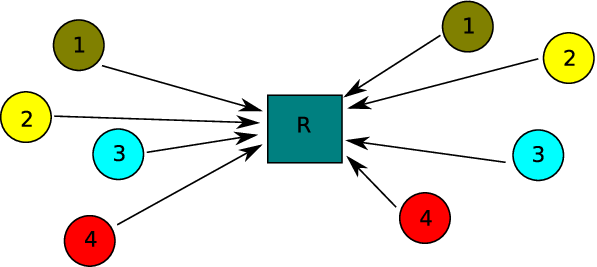

In this paper, we analyze the broadcasting step by using linear and nonlinear precoding strategies at the relay. For simplicity, we assume that the first hop was successful, i.e. all messages were received with an asymptotically small error probability. This assumption is valid given the rates are within the MAC capacity region in the first hop and the first hop does not pose a bottleneck for the system. The resulting communication scenario is illustrated in Fig. 2 for the two-pair case. In this case, the relay has in total four independent messages, given by , and . Obviously, each node is aware of its own message which was transmitted in the first hop. Furthermore, each node is interested in the message from the other node belonging to the same pair, illustrated by .

From the information available at the receivers, it becomes clear that this problem distinguishes itself from a multicast setup, in which a common information is broadcasted to a group of receivers without a priori information at the receivers. For the same reason, it is also different from the well studied broadcast channel. We would also like to emphasize that there are in total pairs of nodes, i.e. we have nodes in total, while the relay is only equipped with antennas. As a consequence, complete interference avoidance using zero-forcing transmission is not possible.
In the following, we are dealing basically with two optimization problems. In the first optimization problem, we are optimizing a weighted sum-rate subject to a transmit power constraint at the relay. In the second optimization problem, we minimize the total transmitted power from the relay under a minimum requirement for each node. For both optimization problems we consider a linear as well as a non-linear precoding strategy.
III Maximizing sum rate
We start with the linear strategy.
III-A Linear techniques
Using linear precoding at the relay, the received signal at node is given by
| (1) | ||||
| (2) |
where is the power allocation to node-pair , is the unit-norm beamformer for node-pair , describes the channel to the -th node, , of node-pair . The channels between the relay and the nodes are modeled as complex Gaussian random variables, i.e. . The relay has an power constraint , is the additive white Gaussian noise with variance at the -th node of node-pair . Thus, the transmit signal is of the form
| (3) |
where is the complex valued signal denoting the information signal for node-pair . The received at node is
| (4) |
It has been shown in [6, 19] for the special case of one pair, that the capacity region can be characterized by its boundary which corresponds to the weighted sum rate given by
| (5) |
with weights and , where .
Thus, using (5) and treating the multi-user interference as noise, the sum rate can be characterized for the general case by
| (6) |
For the two pair case the sum rates of each pair are given by
In the following paragraph, we are deriving the rate expressions achievable with non-linear precoding, namely dirty paper coding. We then describe the choice of beamforming using non-linear precoding with the goal of maximizing the weighted sum rate subject to power constraints. The differences in the expressions for linear precoding are described along with the discussion on the algorithm.
III-B Dirty-Paper Techniques
With dirty-paper coding [18], we are able to pre-compensate the interference since it is already known at the transmitter. By assuming an arbitrary but fixed encoding order, the of user of pair is given by
| (7) |
Thus, we have the following rate vector , where the individual sum rates for each pair are given by
| (8) |
The dirty rate paper region is then given by
| (9) |
which is the the convex hull of the union of all rate vectors over all powers and over all permutations .
Assuming that the interference of the other nodes in (7) and (8) can be regarded as Gaussian, in our approach the beamforming vectors are computed very efficiently for a given order of precoding in the following successive way. First of all, from expression (7), we observe that the node pair encoded last experiences no interference from the other nodes.
Thus, using the approach in [19] the beamforming vector for the node pair is obtained by
| (10) |
with , , and . The weight can be used to prioritize one of the nodes. Intuitively, the beamforming vector in (10) represents a linear combination (up to a phase adjustment) of maximum-ratio transmission beamformers in the direction of the node pairs.
The node pair is considered next. The node pair observes interference from the beam intended for the node pair , which is exactly known. Assuming again that the interference from the node-pair can be regarded as additional white Gaussian noise then the overall interference plus noise (referred to as effective noise in the following) is distributed as with
| (11) |
we compute the beamforming vector for node pair very efficiently as in (10).
This process is continued until is determined. The above algorithm has to be repeated for all possible user orderings . In the linear precoding case, each receiver is observing interference from all other beams in the system, thus the effective noise variance (11) is changed accordingly. The beamformers are obtained by evaluating (10) accordingly. Note that there is no claim of optimality in terms of achievable rates of the beamforming and precoding approaches discussed above. Due to the non-convex structure of the optimization problem, an optimal beamforming strategy for the weighted rate maximization is difficult to obtain. However, note that beamforming has always the advantage of simple processing at the transmitter (scalar instead of vector coding) and receiver (single stream decoding) and is thus often considered in wireless standards such as LTE and WiMAX, which justifies the analysis of such schemes. As an alternative to the approach discussed above, in the following section the equivalent problem of power minimization subject to quality-service-constraints (QoS) in terms of required is considered, first for the linear precoding case, followed by non-linear precoding.
IV Minimizing power
IV-A Linear techniques
In the following, we will show that the uplink-downlink duality [20, 21] does not hold in the setup considered here. We start with the downlink. The optimization problem by using linear precoding is given by
| min. | (12) | |||
| s.t. | ||||
where is the requirements at node . Let us introduce the following matrices with
| (13) | ||||
| (14) |
Note that the are functions of the beamforming vectors, i.e. , with . Then (12) can be rewritten in the following form
| min. | (15) | |||
| s.t. | ||||
with representing the matrix of requirements, where is the all one vector. The power minimization problem in the dual uplink is given by
| min. | (16) | |||
| s.t. |
Note that at the optimum the constraints are achieved with equality (otherwise, the power corresponding to the constraint for can be reduced such that equality is obtained, which would reduce the power spent and thus would be a contradiction.) In the following, by using a counter-example we show that uplink-downlink-duality does not hold. Consider the case , with , , , and . Then, define the following sets according to the constraints in (15) and (16) for this case
| (17) | ||||
for downlink and uplink, respectively. Note that and similarly for the uplink. The sets are illustrated in Fig. 3.


In Fig. 3(a) (analogously in Fig. 3(b)) there are three relevant intersections, marked with a number , and respectively. The numbers and indicate the minimum of the subset and , respectively. The point indicates the minimum of the . For simplicity, it is assumed that is symmetric (cf. Fig. 3). It follows that is symmetric and so is . Note that the minimum of and are on the same dotted slope line passing through due to duality (since ). The same holds for and . However, as can be seen in the figure it holds not true for and (compare the dotted lines passing through the points ), unless as well, which is in general not the case.
Thus, uplink-downlink duality can not be exploited in order to get a solution for the downlink beamformers as in [20, 21] for the broadcast channel (unless the requirements are equal for all nodes, which is a case of limited interest).
However, the optimization problem in (12) can be solved approximately by using a semidefinite relaxation. Let us define . In the original problem, the , , are rank-constraint. This non-convex constraint can be replaced by a convex constraint , where the notation means is a positive semidefinite matrix. While the original constraint was of rank , the can be of any rank with this relaxation. Thus, the relaxed problem is a semidefinite programming problem (SDP) given by
| minimize | (18) | |||
| subject to | (19) | |||
| (20) |
The solution to the relaxed SDP (18) gives a lower bound of the objective function and a relaxed solution . However, if that solution is of rank , then the solution to the relaxed optimization problem is identical to the solution of the original problem. In general, however, the solution will not have rank . As an heuristic but efficient approach, here the eigenvectors corresponding to the largest eigenvalue of are used as a rank approximation.
IV-B Dirty-paper techniques
The procedure here is similar to the linear beamforming case, except that the order of encoding is an additional parameter which has to be taken into account in the optimization. The SDP relaxation in the case of non-linear precoding is given by
| minimize | (21) | |||
| subject to | (22) | |||
| (23) |
Once the optimal beamformers are obtained from (21), a rank approximation is obtained using the same procedure as in the linear case. By defining the requirements in terms of rates as follows
| (24) |
with , we can apply an iterative (bisection) [22] power minimization problem to get an achievable rate region. The parameter is changed at each iteration, i.e. the value of is incremented in the next iteration if (21) is feasible otherwise decreased. The step size is obtained by bisection between the last feasible value of , which is initially equal to zero, and the last infeasible value of , which can be chosen as twice the capacity in the single-pair case given in (5) for initialization. The iterations continue until a predefined accuracy is achieved.
V Illustration
In this section, the results are illustrated by means of numerical simulations. Due to the similarity of the results, we focus in this section on the non-linear precoding strategy, i.e. dirty-paper coding. In Fig. 4, the rate region of a two pair network is shown for a dB. Note that on the coordinate we have the sum rate of pair , while on the ordinate we have the sum rate of pair . Thus, the figure is a projection of a four-dimensional rate region to a two-dimensional one. For both curves in the plot, dirty-paper coding is used. As beamforming strategy the single-pair beamforming approach (cf. (10)) is used and compared to an exhaustive search over a huge set of randomly generated beams. The channel vectors used in the plots have the following norms: , and . From the figure, we observe that the single-pair approach performs very close to the exhaustive search.

The same strategies are compared in Fig. 5, now for dB. Here, we observe a small gap between the single-pair approach and the exhaustive search. Still, the single-user strategy performs reasonably well.

The next Fig. 6 shows the performance of the two strategies for dB. In addition to this, the region obtained using the relaxation method given in (21) is plotted. From the figures, we observe that the gap between the exhaustive search and the single-pair approach has increased further. The region obtained using the relaxation method is comparable to the one using the single-pair approach. From the figures, we conclude that our approach is close to the exhaustive search for low and average , but is suboptimal for high .

VI Conclusion
In this paper, we have addressed the problem of a multi-user relay network, where multiple single-antenna node pairs want to exchange information by using a multiple antenna relay node. In the first step, the nodes transmit their data to the relay, while in the second step, the relay is broadcasting the data by using linear and non-linear precoding strategies. We focused on the broadcasting step and first considered the problem of maximizing the overall rate achievable using linear and dirty-paper type precoding strategies at the relay. Then, we considered the problem of minimizing the total power at the relay subject to individual constraints. We showed that the downlink-uplink duality does not hold for the setup considered here. We also showed that using the beamforming strategy which is optimal in the single-pair case performs very well for practically relevant values of .
References
- [1] G. Kramer, M. Gastpar, and P. Gupta, “Cooperative strategies and capacity theorems for relay networks,” IEEE Trans. Inf. Theory, vol. 51, no. 9, pp. 3037–3063, September 2005.
- [2] I. Maric, R. Dabora, and A. Goldsmith, “On the capacity of the interference channel with a relay,” Proc. of IEEE ISIT 2008, Toronto, Canada, 2008.
- [3] C. E. Shannon, “Two-way communication channels,” Proc. 4th Berkeley Symp. Math. Statistics Probability, Berkeley, CA, pp. 611–644, 1961.
- [4] B. Rankov and A. Wittneben, “Achievable rate regions for the two-way relay channel,” ISIT, Seattle, USA, July 9-14, 2006.
- [5] D. Gündüz and E. Tuncel and J. Nayak, “Rate regions for the separated two-way relay channel,” 46th Allerton Conf. On Comm., Control, and Computing, USA, Sept 23-26 2008.
- [6] Rafael F. Wyrembelski, Tobias J. Oechtering, Igor Bjelakovic, Clemens Schnurr, and Holger Boche, “Capacity of Gaussian MIMO Bidirectional Broadcast Channels,” in Proc. IEEE International Symposium on Information Theory (ISIT ’08), Toronto, Canada, July 2008, pp. 584–588.
- [7] T.J. Oechtering, C. Schnurr, I. Bjelakovic, and H. Boche, “Broadcast Capacity Region of Two-Phase Bidirectional Relaying,” IEEE Transactions on Information Theory, vol. 54, no. 1, pp. 454–458, Jan. 2008.
- [8] I. Hammerström, M. Kuhn, C. Esli, J. Zhao, A. Wittneben, and G. Bauch, “MIMO two-way relaying with transmit CSI at the relay,” IEEE SPAWC 2007, p. 5, June 2007.
- [9] A.S. Avestimehr, A.Sezgin, and D.N.C. Tse, “Approximate capacity of the two-way relay channel: A deterministic approach,” 46th Allerton Conf. On Comm., Control, and Computing, 2008.
- [10] R. Vaze and Jr. R. W. Heath, “Capacity scaling for MIMO two-way relaying,” IEEE Trans. on Signal Processing, submitted, vol. 1, pp. 448–452, April 2008.
- [11] D. Gündüz, O. Simeone, A.J. Goldsmith, H.V. Poor, and S. Shamai, “Multiple multicasts with the help of a relay,” submitted to Transactions on Information Theory, available at http://arxiv.org/abs/0902.3178, 2009.
- [12] D. Gündüz, A. Yener, A.J. Goldsmith, and H.V. Poor, “The multi-way relay channel,” submitted to Transactions on Information Theory, available at http://arxiv.org/abs/1004.2434, 2010.
- [13] M. Chen and A. Yener, “Multiuser two-way relaying for interference limited sytems,” Proc. of IEEE ICC 2008, Beijing, China, May 2008.
- [14] M. Chen and A. Yener, “Interference management for multiuser two-way relaying,” Proc. of IEEE CISS 2008, Princeton, NJ, March 2008.
- [15] A.S. Avestimehr, M.A. Khajehnejad, A. Sezgin, and B. Hassibi, “Capacity region of the deterministic multi-pair bi-directional relay network,” IEEE ITW 2009, Volos, Greece, June 10-12, 2009.
- [16] A.S. Avestimehr, Wireless Network Information Flow: A Deterministic Approach, Ph.d. thesis, UC Berkeley, 2008.
- [17] A. Sezgin, M.A. Khajehnejad, A.S. Avestimehr, and B. Hassibi, “Approximate capacity region of the two-pair bi-directional gaussian relay network,” IEEE ISIT 2009, Seoul, Korea, June 28- July 3, 2009.
- [18] M.H.M. Costa, “Writing on dirty paper (corresp.),” IEEE Transactions on Information Theory, vol. 29, pp. 439–441, May 1983.
- [19] T.J. Oechtering, R.F. Wyrembelski, and H. Boche, “Optimal Transmit Strategy for the 2×1 MISO Bidirectional Broadcast Channel,” in Proc. 9th IEEE Workshop on Signal Processing Advances in Wireless Communications (SPAWC ’08), Recife, Brazil, July 2008.
- [20] H. Boche and M. Schubert, “An general duality theory for uplink and downlink beamforming,” Proc. IEEE VTC 2002 Fall, pp. 87–91, Sep. 2002.
- [21] P. Viswanath and D.N.C. Tse, “Sum capacity of the vector gaussian broadcast channel and uplink downlink duality,” IEEE Trans. on Info. Theory, vol. 49, no. 8, pp. 1912– 1921, Aug. 2003.
- [22] S. Boyd and L. Vanderberghe, Convex optimization, Course reader for EE364 (Stanford) and EE236 (UCLA).