Logic, Reasoning under Uncertainty
and Causality

Logic is the most important framework of reasoning (under certainty). Here, it is rephrased in set-theoretic terms¹¹ 1 Strictly speaking, this set-theoretic logic is “a logic within logic”, since set theory is based on standard logic.. As will be seen, this facilitates its extension to a framework for reasoning under uncertainty.

Let $\Omega$ be a set of outcomes, which is assumed to be finite for simplicity. A subset $A\subset\Omega$ is an event. Let ^c, $\cup$ and $\cap$ be the set-operations of complement, union and intersection respectively. Let $\mathcal{F}$ be an algebra, i.e. a set of events obeying the axioms

• A1.

  $\mathcal{F}\neq\varnothing$.

• A2.

  $A\in\mathcal{F}\hskip 10.00002pt\Rightarrow\hskip 10.00002ptA^{c}\in\mathcal{F}$.

• A3.

  $A,B\in\mathcal{F}\hskip 10.00002pt\Rightarrow\hskip 10.00002ptA\cup B\in\mathcal{F}$.

In this framework, an outcome $\omega\in\Omega$ is a state of affairs and an event $A\in\mathcal{F}$ is a proposition. Hence, a singleton $\{\omega\}\in\mathcal{F}$ is an irreducible (i.e. atomic) proposition about the world. The set-operations ^c, $\cup$ and $\cap$ correspond to the logical connectives of $\neg$ (negation), $\vee$ (disjunction) and $\wedge$ (conjunction) respectively. They allow the construction of complex propositions from simpler ones. An algebra is a system of propositions that is closed under negation and disjunction (and hence is closed under conjunction as well), i.e. it comprises all propositions that the reasoner might entertain.

The objective of logic is to allow the reasoner to conclude the veracity of events given information. Let $\mathcal{V}:=\{1,0,?\}$ be the set of truth states, where 1 is true, 0 is false, and ? is uncertain (but known to be either true or false). From these, $\{1,0\}$ are called truth values. The truth function is the set function $\mathbf{T}$ over $\mathcal{F}\times\mathcal{F}$ defined as

Furthermore, define the shorthand $\mathbf{T}(A):=\mathbf{T}(A|\Omega)$. The quantity $\mathbf{T}(A|B)$ stands for the “truth value of event $A$ given that event $B$ is true”. Accordingly, the knowledge of the reasoner about the facts of the world is represented by his truth function and his algebra. From his point of view, a proposition can be either true, false or uncertain (i.e. having an unresolved truth value given his knowledge). Understanding the definition of the truth function is straightforward. Claiming that an event $B\in\mathcal{F}$ is true means that one of its members $\omega\in B$ is the current outcome/state of affairs. Hence the veracity of $A$ given $B$ is evaluated as follows (Figure 1): if $A$ contains every outcome in $B$ then it must be true as well; if $A$ is known not to contain any of $B$’s outcome then it must be false; and if $A$ contains only part of $B$ then it cannot be resolved, since knowing that $\omega\in B$ does neither imply that $\omega\in A$ nor $\omega\in A^{c}$. The definition of a truth space follows.

The intuitive meaning of a truth space is as follows. Nature arbitrarily selects an outcome $\omega\in\Omega$. (This choice is not governed by a generative law.) Subsequently, the reasoner performs a measurement: he chooses a set $B$ and nature reveals to him whether $\omega\in B$ or not. Accordingly, the reasoners infers the veracity of any event $A\in\mathcal{F}$ by evaluating either $\mathbf{T}(A|B)$ (if $\omega\in B$) or $\mathbf{T}(A|B^{c})$ (if $\omega\notin B$).

Several measurements are combined as a conjunction. Thus, if the reasoner learns that $\omega$ is in $B_{1}$, $B_{2}$, …, and $B_{t}$ after performing $t$ measurements, then the truth value is $\mathbf{T}(A|B_{1}\cap\cdots\cap B_{t})$ for any $A\in\mathcal{F}$.

Unlike logic, Bayesian probability theory allows reasoning under uncertainty. For this end, it provides a consistent mechanism to replace the uncertainty state ${?}$ with a numerical value in the interval $[0,1]$ representing degrees of truth, belief or plausibility.

The goal is to find a suitable definition of a quantity $\mathbf{B}(A|B)$ meaning “the degree of belief in event $A$ given that event $B$ is true” that is consistent with the truth function when it is certain, i.e. $\mathbf{B}(A|B):=\mathbf{T}(A|B)$ if $\mathbf{T}(A|B)\in\{0,1\}$. Consider the three situations in Figure 2. (a) In the case $A\cap B=\varnothing$, we impose $\mathbf{B}(A|B):=\mathbf{T}(A|B)=0$. (b) In the case $B\subset A$, we impose $\mathbf{B}(A|B):=\mathbf{T}(A|B)=1$. (c) In the intermediate case where $\mathbf{T}(A|B)={?}$, the event $A$ only partially covers the members of $B$. If one interprets the quantity $\mathbf{B}(C|D)$ as “the fraction of $D$ contained in $C$”, then one can characterize $\mathbf{B}(A|B)$ with the relation

as long as $\mathbf{B}(B|\Omega)>0$. It is easy to see that this formula generalizes correctly to the border cases, since $\mathbf{B}(A|B)=\frac{0}{\mathbf{B}(B|\Omega)}=0$ when $A\cap B=\varnothing$ and $\mathbf{B}(A|B)=\frac{\mathbf{B}(B|\Omega)}{\mathbf{B}(B|\Omega)}=1$ when $B\subset A$. Noting that $B=B\cap\Omega$ and rearranging terms, one gets

This relation should hold under any restriction to a “universal” set $C\in\mathcal{F}$, not only when it is restricted to $\Omega$. Thus, replacing $\Omega$ by $C$ one obtains

which is known as the product rule for beliefs. Following a similar reasoning, we impose that for any event $A\in\mathcal{F}$, the sum of the degree of belief in $A$ and its complement $A^{c}$ must be true under any condition $B$, i.e.

which is known as the sum rule for beliefs. In summary, we impose the following axioms for beliefs.

Furthermore, define the shorthand $\mathbf{B}(A):=\mathbf{B}(A|\Omega)$. Axiom B1 states that degrees of belief are real values in the unit interval $[0,1]$. Axioms B2 and B3 equate the belief and the truth function under certainty. Axioms B4 and B5 are the structural requirements under uncertainty discussed above. Accordingly, one defines a belief space as follows.

The intuitive meaning of a belief space is analogous to a truth space. Nature arbitrarily selects an outcome $\omega\in\Omega$. Subsequently, the reasoner performs a measurement: he chooses a set $B$ and nature reveals to him whether $\omega\in B$ or not. Accordingly, the reasoners infers the degree of belief in any event $A\in\mathcal{F}$ by evaluating either $\mathbf{B}(A|B)$ (if $\omega\in B$) or $\mathbf{B}(A|B^{c})$ (if $\omega\notin B$).

An easy but fundamental result is that the axioms of belief are equivalent to the axioms of probability²² 2 More precisely, the axioms of beliefs as stated here imply the axioms of probability for finitely additive measures over finite algebras. Furthermore, the axioms of beliefs also specify a unique version of the conditional probability measure.. This simple observation is what constitutes the foundation of Bayesian probability theory.

We now return to the central topic of this chapter. Suppose the reasoner has uncertainty over a set of competing hypotheses about the world. Subsequently, he makes an observation. He can use this observation to update his beliefs about the hypotheses. The following theorem explains how to carry out this update.

The interpretation is as follows. The $H_{1},\ldots,H_{N}$ represent $N$ mutually exclusive hypotheses, and the event $D$ represents an new observation or data. Initially, the reasoner holds a prior belief $\mathbf{B}(H_{n})$ over each hypothesis $H_{n}$. Subsequently, he incorporates the observation of the event $D$ and arrives at a posterior belief $\mathbf{B}(H_{n}|D)$ over each hypothesis $H_{n}$. Bayes’ rule states that this update can be seen as combining the prior belief $\mathbf{B}(H_{n})$ with the likelihood $\mathbf{B}(D|H_{n})$ of observation $D$ under hypothesis $H_{n}$. The denominator $\sum_{m}\mathbf{B}(D|H_{m})\mathbf{B}(H_{m})=\mathbf{B}(D)$ just plays the rôle of a normalizing constant (Figure 3).

Bayes’ rule naturally applies to a sequential setting. Incorporating a new observation $D_{t}$ after having observed $D_{1},D_{2},\ldots,D_{t-1}$ updates the beliefs as

where for the $t$-th update,

play the rôle of the prior belief and the likelihood respectively. Note that

and hence each hypothesis $H_{n}$ naturally determines a probability measure $\mathbf{B}(\cdot|H_{n})$ over sequences of observations.

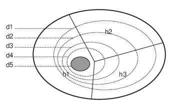
A smaller event $D$ corresponds to a more “accurate” observation. Hence, making a new observation $D^{\prime}$ necessarily improves the accuracy, since

In some cases, the accuracy of an observation (or sequence of observations) can be so high that it uniquely identifies a hypothesis (Figure 4).

The way Bayes’ rule operates can be illustrated as follows. Consider a partition $\{X_{1},\ldots,X_{K}\}$ of $\Omega$ and let $H_{\ast}\in\{H_{1},\ldots,H_{N}\}$ be the true hypothesis, i.e. the outcome $\omega\in\Omega$ is drawn obeying propensities described by $\mathbf{B}(\cdot|H_{\ast})$. The $X_{k}$ represent different observations the reasoner can make. If $\omega$ is drawn and reported to be in $X_{k}$, then the log-posterior probability of hypothesis $H_{n}$ is given by

This decomposition highlights all the relevant terms for understanding Bayesian learning. The term $l_{n}$ is the log-likelihood of the data $X_{k}$. The term $p_{n}$ is the log-prior of hypothesis $H_{n}$, which is a way of representing the relative confidence in hypothesis $H_{n}$ prior to seeing the data. In practice, it can also be interpreted as (a) a complexity term, (b) the log-posterior resulting from “previous” inference steps, or (c) an initialization term for the inference procedure. The term $c$ is the log-probability of the data, which is constant over the hypotheses, and thus does not affect our analysis. Hence, log-posteriors are compared by their differences in $l_{n}+p_{n}$. Ideally, the log-posterior should be maximum for the true hypothesis $H_{n}=H_{\ast}$. However, since $\omega$ is chosen randomly, the log-posterior $\log\mathbf{B}(H_{n}|X_{k})$ is a random quantity. If its variance is high enough, then a particular realization of the data can lead to a log-posterior favoring some “wrong” hypotheses over the true hypothesis, i.e. $l_{n}+p_{n}>l_{\ast}+p_{\ast}$ for some $H_{n}\neq H_{\ast}$. In general, this is an unavoidable problem (that necessarily haunts every statistical inference method). Further insight can be gained by analyzing the expected log-posterior:

This reveals³³ 3 For $p_{i},q_{i}$ probabilities, $\sum_{i}p_{i}\log q_{i}$ is maximum when $q_{i}=p_{i}$ for fixed $p_{i}$. that, on average, the log-likelihood $L_{n}$ is indeed maximized by $H_{n}=H_{\ast}$. Hence, the posterior belief will, on average, concentrate its mass on the hypotheses having high $L_{n}+P_{n}$.

There is one technical point that merits closer inspection. Consider two events $A,B\in\mathcal{F}$ such that $B\cap A\neq\varnothing$ but $\mathbf{B}(B)=0$. One has that

due to the definition of the truth function and due to Axiom B4. From this, we conclude that $\mathbf{B}(A\cap B)=0$. For $\mathbf{B}(A|B)$ there are two possible cases. If $B\subset A$, then $\mathbf{B}(A|B)=1$ due to Axiom B2. However, if $B\not\subset A$, then $\mathbf{B}(A|B)$ is independent of the degree of belief $\mathbf{B}(C)$ of any event $C\in\mathcal{F}$. More generally, if $D\in\mathcal{F}$ is such that $\mathbf{B}(B|D)=0$, then the value of $\mathbf{B}(A|B)$ is independent of the degree of belief $\mathbf{B}(C|D)$ of any event $C\in\mathcal{F}$.

The bottom line is that conditioning on an event with zero belief is a well-defined operation under the belief axioms outlined in Definition 2. This is not so in the case of the probability axioms of measure theory. In measure theory, the probability measure is a global measure $\mu$ over $\mathcal{F}$, i.e. a function assigning probability mass $\mu(A)$ to any event $A\in\mathcal{F}$. However, implicit in this definition is the fact that these masses are measured w.r.t. the certain event $\Omega$. Because of this, the information contained in the probability measure $\mu$ is insufficient to uniquely determine the conditional probability measure $\mu(\cdot|B)$ arising from conditioning on an event $B\in\mathcal{F}$ having $\mu(B)=0$. In contrast, the belief function $\mathbf{B}$ is a well-defined measure w.r.t. any conditioning event $B\in\mathcal{F}$, i.e. assigning probability mass $\mathbf{B}(A|B)$ to any event $A\in\mathcal{F}$.

References

- Cox [1961] R.T. Cox. The Algebra of Probable Inference. Johns Hopkins, 1961.
- Dawid [2010] A. P. Dawid. Beware of the DAG! Journal of Machine Learning Research, (to appear), 2010.
- Jaynes and Bretthorst [2003] E.T. Jaynes and L.G. Bretthorst. Probability Theory: The Logic of Science: Books. Cambridge University Press, 2003.
- Pearl [2000] J. Pearl. Causality: Models, Reasoning, and Inference. Cambridge University Press, Cambridge, UK, 2000.
- Shafer [1996] G. Shafer. The art of causal conjecture. The MIT Press, 1996.
- Spirtes et al. [2000] P. Spirtes, C. Glymour, and R. Scheines. Causation, Prediction and Search. Springer-Verlag, New York, 2nd edition, 2000.