An equivalence between a Maximum Caliber analysis of two-state kinetics and the Ising model

The Maximum Entropy (MaxEnt) formalism provides an alternative to more conventional statistical mechanics approaches by offering a convenient jumping off point for thinking about problems that are not within the purview of equilibrium statistical mechanics. For non-equilibrium systems, the corresponding idea is called the Principle of Maximum Caliber (MaxCal), in which we attempt to determine the probability that a particle travels on a particular space-time path rather than its probability of occupying a certain energy level [7]. One way to think about these information-theoretic approaches is that the probability distributions generated by MaxEnt and MaxCal are the least-biased inferences about the distributions that can be made on the limited information that is in hand; i.e., by maximizing the Shannon entropy over the collection of possible outcomes for the system of interest [15]. MaxEnt has been used for several decades to model everything from neural firing [13] to climate change [10] and many applications between. MaxCal has been subjected to a few applications including analysis of the dynamics of a two-state system [16, 17] and to examine the origin of phenomenological transport laws including Fick’s law of diffusion [14] and fluctuation theorems [1].

The MaxCal approach is relatively unexplored and has been set forth as a very general method of analyzing nonequilibrium systems [7, 9, 8]. By applying MaxCal to experimentally realizable systems, we hope that we can not only make useful predictions of the behavior of concrete experimental systems, but also help identify and highlight the outstanding theoretical questions that impede progress towards practical use of MaxCal. One such system that we find appealing is the dynamics of a two-state system, partly because of its simplicity and because of the opportunity to manipulate such systems experimentally. To that end, in this paper, we analyze the dynamics of a two-state system, cognizant that it is only one concrete application of the MaxCal approach and that much remains to be done to demonstrate MaxCal’s usefulness more generally.

MaxEnt as used in equilibrium statistical mechanics and MaxCal exploit almost entirely the same theoretical prescription, except that MaxEnt as used in equilibrium statistical mechanics identifies the entropy-maximizing probability distribution of particle occupancy over energy states, whereas MaxCal identifies the caliber-maximizing probability distribution of particle occupancy over possible space-time paths (“microtrajectories”). Caliber is an entropy-like quantity that has the same form as the Shannon entropy, ${\cal C}=\sum_{\Gamma}p_{\Gamma}\ln p_{\Gamma}+\sum_{i}\lambda_{i}\langle A_{i}\rangle_{\Gamma}$. In this equation, ${\cal C}$ is the caliber, $p_{\Gamma}$ denotes the probability of a given microtrajectory $\Gamma$, and each $\langle A_{i}\rangle_{\Gamma}$ is a macroscopic observable which serves as a constraint within the information-theoretic approach. For convenience, we will denote an average over the microstates $\langle A_{i}\rangle_{\Gamma}$ as $\langle A_{i}\rangle$. The constants $\lambda_{i}$ are Lagrange multipliers corresponding to those constraints. Maximizing the caliber yields a full probability distribution for all the allowed microtrajectories.

In this paper, we analyze the dynamics of the two-state system using a MaxCal model and derive new insights into MaxCal and the discretized two-state system in the process. The organization of this paper is as follows. Background on MaxCal is presented in Section II. In Section III, we show that the dynamics of a two-state system are mathematically equivalent to the 1-D Ising model, and that there are different but equivalent ways of picking the MaxCal constraints. In Section IV, we use simulation to investigate the relationship between the MaxCal model for the two-state system proposed here and a previously proposed MaxCal model for the two-state system [16, 17].

As noted above, caliber is an entropy-like quantity that increases as the relative probabilities of the microtrajectories becomes less predictable. As a result of maximizing the caliber, MaxCal asserts that our best guess as to the probability of observing a particular microtrajectory $\Gamma$ is

where

is a normalization factor dubbed by Jaynes as the “partition functional” and the $A_{i,\Gamma}$ are values of macroscopic observables $A_{i}$ along the microtrajectory labeled $\Gamma$. $\lambda_{i}$ are the corresponding Lagrange multipliers that can be calculated from $\langle A_{i}\rangle=\frac{\partial\ln Z}{\partial\lambda_{i}}$ [7].

A distinguishing feature of MaxCal-derived formulas of nonequilibrium statistical mechanics as compared to more conventional nonequilibrium statistical mechanics formulas, e.g. the Jarzynski equality [6], is that MaxCal solves an inverse problem, in which we infer microscopic properties based on macroscopic observations. The MaxCal distribution described in Equation 1 is typically generated on the basis of knowing only a small number of macroscopic observables $\langle A_{i}\rangle$ and predicts the probability of traveling any one of the many possible microtrajectories $\Gamma$. For example, in the two-state systems simulated in this paper which each have $10^{5}$ time steps, only two macroscopic observables are used to generate predictions for the probability of traversing the entirety of the $2^{10^{5}}$ possible microtrajectories. However, since the average probability of observing a particular microtrajectory is typically very small, it is difficult to obtain accurate experimental estimates of $p_{\Gamma}$ itself to which we can compare MaxCal predictions. Instead, to test the accuracy of a MaxCal model, we can predict higher order moments of the joint probability distribution $p(A_{1},A_{2},...,A_{n})$. These higher moments are more robust than individual microtrajectory probabilities $p_{\Gamma}$ to the depth of our experimental investigation of the system. Again, note that these higher moments are not used in any way to determine the probability distribution $p(A_{1},...,A_{n})$ itself. Rather, they are predictions about more nuanced features of the two-state system than those simple average quantities used to establish the distribution given in Equation 1.

The dynamics of the two-state system can be completely characterized by rate equations in terms of the constants $k_{A}$ and $k_{B}$, where $k_{A}$ and $k_{B}$ are the intrinsic rate constants for transition from state A to state B and vice versa [2]. Indeed, one of the interesting outcomes of the present paper is a simple relation between the conventional rate constants and the Lagrange multipliers that are central to the MaxCal description of the same system.

To make the dynamics of the two-state system amenable to simple MaxCal analysis, let the MaxCal trajectory $\Gamma$ be a string of $1$’s and $-1$’s describing the state of the system as a function of time. More explicitly, suppose that our two-state system is a particle jumping between wells on a double-well potential energy landscape, examples of which are shown in Figure 1. Let $\sigma_{\Gamma}(t)$ represent the system’s state at time $t$. If the particle is in the left potential well at time $t$, then we say it is in state $A$ and that $\sigma_{\Gamma}(t)=1$; if the particle is in the right potential well at time $t$, then we say it is in state $B$ and $\sigma_{\Gamma}(t)=-1$. Thus, a particle’s trajectory $\Gamma$ is equivalent to a series of $N$ $1$’s and $-1$’s, for which the particle’s state is sampled every $\Delta t$ and the total time spent observing the particles of interest is $N\Delta t$.

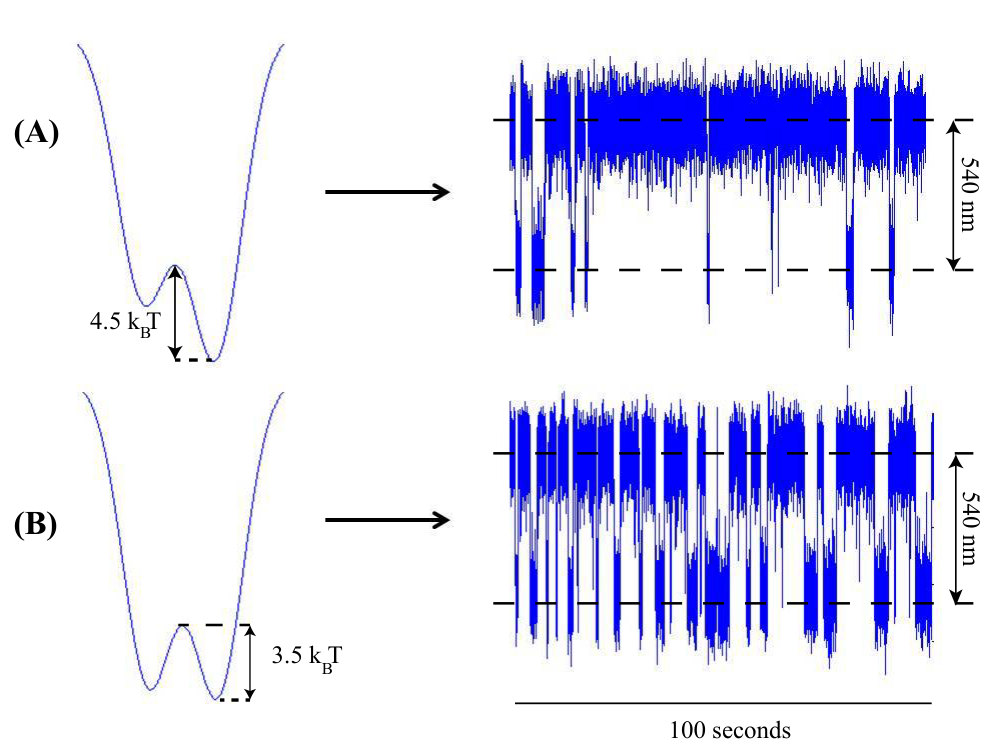
This discretized picture of the two-state process will lead to accurate calculations only if our time step $\Delta t$ is small enough to capture nearly all state transitions [4]. In other words, in the language of rate constants, we require that the average waiting time in both states is much larger than the time step $\Delta t$. For Markov systems, the waiting time in a particular state $t$ follows an exponential distribution with a mean of $\langle t\rangle=\frac{1}{k}$ [2]. Thus, here, we require $\Delta t<<\frac{1}{k_{A}},~\frac{1}{k_{B}}$, or identically $k_{A}\Delta t,~k_{B}\Delta t<<1$ as described previously [17]. If this heuristic condition is satisfied, missed transitions are negligible. For the two-well potential landscapes considered here, waiting times range from $0.5$ to $5$ s, whereas $\Delta t=1$ ms.

We wish to test our MaxCal model by comparing theoretical predictions to data obtained from simulations or experimental measurements of a two-state system. In an earlier paper, we described the use of a dual-well optical trap that could be used to sculpt different two-state trajectories by tuning the properties of the adjacent wells [17]. In this paper, we continue along similar lines, but instead using simulated data for this system like that shown in Figure 1. Trajectories were simulated according to the Langevin equation subject to an external potential [3],

where $U(x)$ is a potential of the form

meant to mimic the two-well landscape imposed by the optical traps. The parameters $\mu_{1}$ and $\mu_{2}$ give the x-coordinates on which each well is centered; the parameters $\sigma_{1}$ and $\sigma_{2}$ refer to the width of each potential well; and $E_{1}$ and $E_{2}$ refer to the depth of each well. In simulations, parameters $\mu_{1}$, $\mu_{2}$, $\sigma_{1}$, and $\sigma_{2}$ were kept constant. However, fifteen different combinations of $E_{1}$ and $E_{2}$ were used to simulate fifteen different double potential wells. See Table 1 and Table 2 for a listing of $E_{1}$, $E_{2}$, and $\Delta E=E_{1}-E_{2}$ for each of the relevant energy landscapes.

The simulations give us explicit realizations of the trajectory distribution that we can compare to theoretical predictions of our MaxCal model via partial derivatives of the partition function. For example, we can compute the fluctuations in the mean state as

Similarly, we can compute other correlation functions of interest such as

and

To test our MaxCal model, we compared moments computed from the simulated data described previously with moments predicted by the MaxCal model as revealed in Equations 30, 31, and 32, for example. Figures 2, 3, and 4 demonstrate good agreement between simulated data and the moments predicted from the MaxCal model via Equations 30, 31, and 32, respectively. The calculations from this MaxCal model are also compared to the calculations from the MaxCal model described in Section III.2 [17]. In these graphs, each data point corresponds to a different potential well setup and error bars correspond to standard error. Uncertainty in calculated values of moments stems from uncertainty in the value of the constraints taken from simulated data. See Appendix I for details.

From Figures 2-4, there is good agreement between the two MaxCal models, which we have already argued are equivalent aside from a difference in boundary conditions. This difference between the moment predictions in Figures 2-4 is barely perceptible because $N=10^{5}>>1$, but there is certainly a significant difference in MaxCal predictions due to boundary conditions when there are very few timesteps [16]. For most cases of interest, the long-time limit will be the relevant situation in which the boundary conditions become less relevant as the total sampling time $N\Delta t$ increases compared to the time step $\Delta t$, just as surface terms become irrelevant in the thermodynamic limit in equilibrium statistical mechanics [11].

This indifference to boundary conditions can also be seen by testing Equations 23 and 24 derived for Lagrange multipliers in Section III.2. Recall that those equations hold only if periodic boundary conditions and exact boundary conditions lead to equivalent results, and therefore any deviation from the equations is due entirely to a difference in boundary conditions. Figures 5 and 6 demonstrate that Equations 23 and 24 agree well with the data from the fifteen different potential well setups described above, although Figure 5 shows a systematic deviation due to a difference in boundary conditions. We calculated rates $k_{A}$ and $k_{B}$ from Equation 25 and the values of the Lagrange multipliers derived using $\frac{\partial\ln Z}{\partial\ln\gamma_{aa}}=\langle N_{aa}\rangle$, $\frac{\partial\ln Z}{\partial\ln\gamma_{bb}}=\langle N_{bb}\rangle$, $\frac{\partial\ln Z}{\partial\ln\gamma_{ab}}=\langle N_{ab}\rangle$, and $\frac{\partial\ln Z}{\partial\ln\gamma_{ba}}=\langle N_{ba}\rangle$. See Appendix II for more details.

The Ising model can also be used for predicting the autocorrelation function for the different states, so that MaxCal model calculations can be compared directly to predictions from the master equations for the two-state (i.e. random telegraph) problem [2]. In the language of the Ising model, the autocorrelation function for being in the state $A$ is

The quantity $\frac{\sigma(t)+1}{2}$ is $1$ when the particle is in state A at time $t$ and $0$ if the particle is in state B; thus, the quantity $(\frac{\sigma(t)+1}{2})(\frac{\sigma(t+\tau)+1}{2})$ acts as a counter that is $1$ when the particle is in state A at times $t$ and $t+\tau$, and $0$ otherwise. Expansion of this expression gives

Similarly, we can write the corresponding autocorrelation function for the other state as

Here $J,~h$ are not time dependent, so that $\langle\sigma(t)\sigma(t+\tau)\rangle$ is the same for any $t$. We can evaluate $\langle\sigma(t)\sigma(t+\tau)\rangle$ by using standard transfer matrix techniques [11], yielding the result

where $T$ is given by Equation (III.1) and $P$ is the Pauli spin matrix $\left(\begin{smallmatrix}1&0\\ 0&-1\end{smallmatrix}\right)$. We find that

where

Recall that $D=\left(\begin{smallmatrix}\lambda_{+}&0\\ 0&\lambda_{-}\end{smallmatrix}\right)$, which makes exponentiation trivial, resulting in

Therefore, matrix multiplication gives

which we can use to directly calculate $P(A,t)$ and $P(B,t)$.

A comparison between simulated and theoretical values for $P(A,t)$ is shown in Figure 7. Equations 34 and 35 are quite accurate, although they are not identical to the probabilities that one would calculate using master equations. The reason for this is that our discrete MaxCal model has a third implicit parameter in addition to $k_{A}$ and $k_{B}$: $\Delta t$, the time scale associated with the discretization of the trajectories. The exact nature of the dependence on $\Delta t$ was made explicit in Section III.2.

There are benefits and drawbacks to using the MaxCal analysis presented here instead of a more traditional master equation analysis. For example, it is straightforward to calculate the joint probability distribution of $N_{s}$ and $i$, $p(N_{s},i)$, using the MaxCal model. Indeed, for some quantities we have not even been able to figure out how to compute them using the master equation treatment. The ease of these calculations in the MaxCal setting results from the fact that the moments of the probability distribution $p(N_{s},i)$ are simply partial derivatives of the partition function $Z$ in our MaxCal model, and in the master equation formalism, one must calculate $p(N_{s},i)$ from $P(A,t)$ and $P(B,t)$. It is straightforward to calculate autocorrelations using the master equation formalism via a linear differential equation; the same quantity can be calculated from MaxCal using transfer matrices.

Both in classical equilibrium thermodynamics and statistical mechanics and in the thermodynamics of small departures from equilibrium, there are broad classes of relations such as the Maxwell relations and the Onsager relations that illustrate the mathematical linkage of quantities that at first blush might seem unrelated. In some cases, the simplest way to explain these relations is that they reflect equality of certain second-order mixed partial derivatives. The maximum caliber formalism admits similar relations [9, 16]. In the language of trajectories, what these relations tell us is that if we have measured properties such as $N_{s}$ and $i$ on one two-well landscape, we can predict what the dynamics will be like on a “nearby” landscape without doing any further measurements.

In this MaxCal model, Maxwell-like relations fall out as the equality of mixed partial derivatives of $\ln Z$. For example, the statement that $\frac{\partial^{2}\ln Z}{\partial h\partial J}=\frac{\partial^{2}\ln Z}{\partial J\partial h}$ leads to

Other results can be obtained from higher-order mixed partial derivatives, e.g. $\frac{\partial^{3}\ln Z}{\partial J\partial^{2}h}=\frac{\partial^{2}}{\partial J\partial h}(\frac{\partial\ln Z}{\partial h})$ yields $-\frac{1}{2}\frac{\partial^{2}\langle N_{s}\rangle}{\partial h^{2}}=\frac{\partial^{2}\langle i\rangle}{\partial h^{2}}$. It still remains to see how to turn such relations into general useful predictive tools for the design and interpretation of experiments.

In summary, we have studied a single colloidal particle undergoing a two-state process with stationary rates, though the problem with time-varying rates is of great interest. This classic problem is studied using the theory of maximum caliber. By measuring relatively short trajectories ($\sim$ one hour), we are able to find the full probability distribution of trajectories from a MaxCal model using the average frequency of state-switching and the average state as constraints, and confirm that the predicted trajectory distribution agrees with simulated data. Additionally, we show that the “Markov-like” constraints used in an earlier MaxCal analysis of the two-state system [17] differs from the MaxCal analysis presented here only via a difference in boundary conditions. The mapping of the Ising-like MaxCal model onto the Markov-like MaxCal model allows us to assign a physical interpretation to the Lagrange multipliers.

Mapping two-state dynamics onto a one-dimensional Ising model yields unexpected insights into two-state dynamics, even though the master equations that describe two-state kinetics have been used for decades. First, we show that the dynamics of the two-state system can be mapped onto a 1-D Ising model whose “coupling constant” and “magnetic field” can be written explicitly in terms of $k_{A}$, $k_{B}$, and $\Delta t$. Then we derive several relationships that hold true specifically for discretized two-state systems, i.e. the expressions depend on the time step $\Delta t$ as well as the rates $k_{A}$ and $k_{B}$. We derive and verify expressions for the moments of the joint probability distribution $p(N_{s},i)$, which to the best of our knowledge have not been derived previously using the traditional master equation formalism or anything else. Next we derive and verify an expression for the autocorrelation functions $P(A,t)$ and $P(B,t)$ in a discretized system. It is possible that these new formulas will be of practical value to those who study systems that can be modeled as two-state systems, e.g. ion channels and ligand-receptor complexes.

We are grateful to Ken Dill and Kings Ghosh for years of discussion on the MaxCal formalism. SM acknowledges the support of a Caltech Student Undergraduate Research Fellowship. DW acknowledges the support of a NIH UCLA-Caltech MD-PhD fellowship. This work was also supported by the NIH Director’s Pioneer award.

Because of the finite time scale of our simulations, there is uncertainty in our simulation measurements of $\langle i\rangle$ and $\langle N_{s}\rangle$; there is a standard error associated with both measurements– $\langle i\rangle\pm\sigma_{i}$ and $\langle N_{s}\rangle\pm\sigma_{N_{s}}$. Recall that the Lagrange multipliers $J$ and $h$ are determined by solving transcendental equations $\frac{\partial\ln Z}{\partial J}=\langle 2N_{s}\rangle$ and $\frac{\partial\ln Z}{\partial h}=\langle i\rangle$. These values must be modified in order to account for standard deviation $\sigma_{N_{s}}$ and $\sigma_{i}$ in our estimation of constraints $\langle N_{s}\rangle$ and $\langle i\rangle$. We can determine the standard deviation of Lagrange multipliers, $\sigma_{J}$ and $\sigma_{h}$, by using error propagation on $\langle i\rangle$ and $\langle N_{s}\rangle$, namely,

and

The error bars in Figures 5 and 6 are the standard devations from Equations 43 and 44.

We can then use Equations (43) and (44) to solve for $\sigma_{h}$ and $\sigma_{J}$. Finding the standard deviation of second moments follows from a similar strategy in error propagation. For instance, $X=\langle i^{2}\rangle-\langle i\rangle^{2}=\frac{\partial^{2}\ln Z}{\partial h^{2}}$. The standard deviation of this quantity is

In this equation, $\frac{\partial^{3}\ln Z}{\partial h^{3}}$ and $\frac{\partial^{3}\ln Z}{\partial J\partial h^{2}}$ can be evaluated at $J$ and $h$, and $\sigma_{J}$ and $\sigma_{h}$ are obtained via Equations (43) and (44). Thus the standard deviation of $\langle i^{2}\rangle-\langle i\rangle^{2}$ can be evaluated. This analysis extends to the other second moments. Let $Y=\langle N_{s}i\rangle-\langle N_{s}\rangle\langle i\rangle=-\frac{1}{2}\frac{\partial^{2}\ln Z}{\partial J\partial h}$ and $Z=\langle N_{s}^{2}\rangle-\langle N_{s}\rangle^{2}=-\frac{1}{2}\frac{\partial^{2}\ln Z}{\partial J^{2}}$. Similar analysis to that above shows:

and

What is plotted in Figures 2-4 and Figure 7 is the standard error, which is the standard deviation divided by $\sqrt{M}$, where $M$ is the number of trajectories simulated. For each different potential surface, $2200$ trajectories were simulated, and so $M=2200$.

Previously in Section IV we saw a systematic underestimation of the measured value of $J$. To understand this, we would like to compare values of $J$ calculated using the same constraints $\langle i\rangle,~\langle N_{s}\rangle$ and same MaxCal model in Equation 8, just with three different types of boundary conditions– exact, periodic, and free. Even though we cannot analytically evaluate the partition function under free boundary conditions, we can still find the value of $J$ under free boundary conditions following methods in earlier work [5]. Under free boundary conditions,

Thus, we can evaluate the Lagrange multiplier $J$ as a function of the constraint $\langle N_{s}\rangle$ using

which, after some straightforward algebra, yields

To recap, we now have three different values for $J$ depending on boundary conditions used to evaluate the same MaxCal partition function in Equation 8. Under periodic boundary conditions, $J$ is found from numerically solving the closed form, transcendental system of equations given by Equations 9 and 10. Under exact boundary conditions, $J$ is given by Equation 23. Under free boundary conditions, $J$ is given by Equation 51. Our goal is to understand whether or not boundary conditions is really driving the difference between the three different $J$’s by examining how the difference between the different $J$’s varies with the constraint $\langle i\rangle$.

The average state $\frac{\langle i\rangle}{N}$ is a sort of metric for how hard the particle is pushed to be in one state or the other. Periodic boundary conditions become more like exact boundary conditions as the driving force to be in either state increases, since then the probability that a trajectory will start and end in the same state increases. Free periodic boundary conditions become more like exact boundary conditions as $|\frac{\langle i\rangle}{N}|$ approaches $0$, since when neither state is preferred, the particle is just as likely to start and end in either state. In Figure 8, as the average state approaches $1$ and $-1$, exact and periodic boundary conditions split away from free periodic boundary condition estimates. For $\langle i\rangle$ close to $0$, the three boundary conditions are very close together. This is what we would expect if boundary conditions were indeed driving the difference between the different Lagrange multiplier values.

References

- [1] R. Dewar. Information theory explanation of the fluctuation theorem, maximum entropy production, and self-organized criticality in non-equilibrium stationary states. J. Phys. A: Math. Gen., 36:631–641, 2003.
- [2] C.W. Gardiner. Handbook of stochastic methods: for physics, chemistry and the natural sciences. Springer, 1985.
- [3] D. T. Gillespie. The multivariate langevin and fokker-planck equations. Am. J. Phys., 64(10):1246–1257, 1996.
- [4] A.G. Hawkes, A. Jalali, and D. Colquhoun. The distributions of the apparent open times and shut times in a single channel record when brief events cannot be detected. Phil. Trans. R. Soc. Lond. A, 332:511–538, 1990.
- [5] M. Inamdar. PhD thesis, Caltech, 2006.
- [6] C. Jarzynski. Nonequilibrium equality for free energy differences. Phys. Rev. Lett., 78(14):2690–2693, 1997.
- [7] E. T. Jaynes. Macroscopic prediction, 1996.
- [8] E.T. Jaynes. Where we stand on maximum entropy? In Maximum Entropy Formalism Conference, 1978.
- [9] E.T. Jaynes. The minimum entropy production principle. Ann. Rev. Phys. Chem., 31:579–601, 1980.
- [10] Karmeshu. Entropy measures, maximum entropy principle and emerging applications. Springer, 2003.
- [11] R.K. Pathria. Statistical Mechanics. Elsevier, 1996.
- [12] R. Phillips and et al. Physical Biology of the Cell. Garland Science, 2009.
- [13] E. Schneidman and et al. Weak pairwise correlations imply strongly correlated network states in a neural population. Nature, 440:1007–1012, 2006.
- [14] E. Seitaridou and et al. Measuring flux distributions for diffusion in the small-numbers limit. J. Phys. Chem. B, 111:2288–2292, 2007.
- [15] C. E. Shannon. A mathematical theory of communication. The Bell System Technical Journal, 27:379–423,623–656, 1948.
- [16] G. Stock, K. Ghosh, and K. A. Dill. Maximum caliber: A variational approach applied to two-state dynamics. J. Phys. Chem., 128:194102–194113, 2008.
- [17] D. Wu and et al. Trajectory approach to two-state kinetics of single particles on sculpted energy landscapes. Phys. Rev. Lett., 103, 2009.