Phase transitions in random Potts systems and the community detection problem: spin-glass type and dynamic perspectives
Abstract
Phase transitions in spin glass type systems and, more recently, in related computational problems have gained broad interest in disparate arenas. In the current work, we focus on the “community detection” problem when cast in terms of a general Potts spin glass type problem. As such, our results apply to rather broad Potts spin glass type systems. Community detection describes the general problem of partitioning a complex system involving many elements into optimally decoupled “communities” of such elements. We report on phase transitions between solvable and unsolvable regimes. Solvable region may further split into “easy” and “hard” phases. Spin glass type phase transitions appear at both low and high temperatures (or noise). Low temperature transitions correspond to an “order by disorder” type effect wherein fluctuations render the system ordered or solvable. Separate transitions appear at higher temperatures into a disordered (or an unsolvable) phase. Different sorts of randomness lead to disparate behaviors. We illustrate the spin glass character of both transitions and report on memory effects. We further relate Potts type spin systems to mechanical analogs and suggest how chaotic-type behavior in general thermodynamic systems can indeed naturally arise in hard-computational problems and spin-glasses. The correspondence between the two types of transitions (spin glass and dynamic) is likely to extend across a larger spectrum of spin glass type systems and hard computational problems. We briefly discuss potential implications of these transitions in complex many body physical systems.
pacs
89.75.Fb, 64.60.Cn, 89.65.-sI Introduction
One of the highly significant recent applications of statistical mechanics concerns a topic of broad interest– that of community detection[1, 2, 3, 4, 5, 6, 7, 9, 10, 8, 11, 12, 13] in complex networks [1, 7, 14] and related computational problems [15, 16, 17]. In this article, we address further development in the challenging quest of studying these difficult computational problems by bringing additional tools from physics into the fore. Our aim is not only to study the community detection problem itself. Rather, we use the community detection problem as a platform for a detailed investigation of phase transitions [19, 20, 18, 21] associated with complex computational problems and, generally, Potts spin glass type systems. Various applications of physics to computational problems have enabled significant advances in the design of new algorithms and the identification and understanding of various “phases” of computational problems in way that has dramatically advanced previous approaches.
In this article, we provide direct evidence for earlier indications of two phase transitions in the community detection problem and more generally in Potts type spin glass systems. These Potts type spin glass transitions occur at both low and high temperatures (or, similarly, at low and high levels of randomness or noise). These transitions reflect different underlying physics. Earlier reports of such transitions were afforded by information theory measures (as in Appendix E of [9]) and a computational “computational susceptibility” to be defined in later sections of the current work that monitors the onset of a large number of local minima, or large computational complexity (as in Appendix B of [10]). As was earlier shown (e.g., Fig. 11 in [10]), overlap parameters (to be defined herein) such as the normalized mutual information exhibit progressively sharper changes as the system size increases. This suggests the existence of bona fide thermodynamic transitions. In this article, we will investigate “fixed” spin glass type Potts Hamiltonian. By “fixed”, we allude new spin glass systems with fixed parameters which are not dependent on the problem itself. Thus, this fixed approach contrasts with, e.g., “modularity” [1, 8, 22] or other models that involved comparisons to random case systems- so called “null models” [1, 8, 11] that have been earlier invoked on in the community detection problem. When cast in terms of canonical fixed Potts spin Hamiltonian, the system exhibits sharper phase transitions [10]. By applying our model to a general random graph, we can locate phase transitions between solvable and unsolvable regions. Solvable regions may further splinter into “easy” and “hard” phases. We further elaborate on disparate phase transitions (at low and high temperatures) in these rather general Potts spin glass type systems.It is noteworthy that a similar analysis can be done for any other method for detecting communities. Within most of the easy phase, all of the known methods agree on the solutions. The results of our analysis are not relevant to only one specific method.
Insofar as the classification of computational problems, the main tools of analysis to date were of a static nature and further invoke various forms of “cavity” type approximations [23, 24] and extremely powerful related approaches such as “belief propagation” [13, 25, 26]. Cavity type methods were of immense success early on in studying mean-field type theories in spin-glasses and, in the last decade, have seen a rapid resurgence in enabling new and very potent algorithms and in better enabling an understanding of complex problems.
In this article, we directly study the phase transition in computational problems such as community detection from both static (i.e., thermodynamic) and dynamic aspects. We directly numerically investigate, sans any analytical approximations, thermodynamic quantities characterizing the transition augmented by further direct measures of the energy landscape of these systems by use of a “computational susceptibility” that we will introduce later on that monitors the increase number of local minima and convergence with local minima. In the dynamic approach, in order to relate hard computational problems to classical dynamics, we will dualize, via a Hubbard-Stratonovich transformation, the original (discrete) system to be optimized by a continuous theory for which equations of motion can be written down and the dynamics investigated. By employing these two complimentary approaches ((i) static thermodynamic of information measures of the energy landscape and (ii) classical dynamics), we correspondingly report on the existence of (i) static spin-glass-type transitions as well as (ii) dynamical transitions, i.e., the transition of nodes from stable orbits to “chaos”. The transitions as ascertained by both approaches occur at precisely the same set of parameters describing the problem. As far as we are aware, earlier studies have not investigated the general phase diagram of this important problem. To date, links between dynamical mechanical transitions and spin-glass type transitions in computational problems such as this have, furthermore, not been discovered.
II Outline
The rest of the paper is organized as follows. In Section III, we introduce the (general) Potts model that will form the focus of our attention and its relation to the community detection problem. In Section IV, we introduce the basic definitions of trials and replicas that are imperative to our approach. These allow us to directly explore the energy landscape of the system without the aid of approximations. This is followed, in Section V, by a review of information theoretic quantities as they pertain to our method. We then proceed to present our findings. In Section VII we present evidence for the existence of spin-glass type transitions that may generally occur at both high and low temperatures. We discuss the physical origin of these transitions and the relation between the phase diagram of the community detection problem (and, more generally, that of the Potts model) to other important computational problems. In Section VIII, we relate the Potts model system to a continuous mechanical system. By examining its dynamics, we note that, in this mechanical system, the transition to chaos onsets exactly at the same set of parameters at which the Potts model displays spin-glass type transitions. Various technical details and further physical aspects have been relegated to the appendices.
III The Potts model
We will employ a, rather general, spin-glass type Potts model Hamiltonian (denoted, henceforth, as the “Absolute Potts Model” (APM)) [9] for solving the community detection problem. The Hamiltonian reads
| (1) |
Here, is an adjacency matrix element which assumes a value of if nodes and are connected and a value of otherwise. The spins attain integer values: . Their values reflect the community membership. That is, if then node belongs to community number . The parameter denotes the total number of communities. To simplify the analysis, we will, unless stated otherwise, set (the so-called resolution parameter [10]) . (In recent work [27], we reported on similar results for general and weighted version of Eq. (1). In particular, in physics related applications for many particle systems, the weights were determined by the two-body interactions [28, 29].)
Although, as we elaborate on in Appendix A, we can achieve analytic solutions for certain cases of graphs (e.g., employing the cavity method [25, 30, 31, 32, 33] when all of the nodes are of a fixed degree of or Ising systems (i.e., systems with communities)), most general graphs (with arbitrary degree and cluster size distributions) require computer simulation. To this end, we will undertake a direct numerical investigation of the system at hand without the need to invoke analytical approximations or assumptions. Our (“zero-temperature”) community detection algorithm for minimizing Eq. (1) was discussed at length in Refs. [9, 10, 28, 29, 27]. In the current work, we investigate the above Hamiltonian of Eq. (1) at zero temperature [9] and also at finite temperatures () with the use of a heat bath algorithm (HBA) (Appendix B). In brief, within the HBA, we will sequentially allow each node an opportunity to change the community membership during each time step with probabilities determined by a Boltzman weight () at a specified temperature and the energy change () as the node were moved to each connected cluster (or to a new cluster). Similarly, as elaborated on in more detail in Appendix B, following each step, we further allow the possibility of community merges based on a Boltzman weight.


IV Definitions: Trials and Replicas
Before turning to the specifics of our results, we need to introduce several basic notions. We start by discussing two concepts which underlie our approach. Both concepts pertain to the use of multiple identical copies of the same system which differ from one another by a permutation of the site indices. In the definitions of “trials” and “replicas” given below, we build on the existence of a given algorithm (any algorithm) that may minimize a given energy or cost function. In our particular case, we minimize the Hamiltonian of Eq. (1). However, these ideas and concepts are more general.
Trials. We use trials alone in our bare community detection algorithm [10, 9]. We run the algorithm on the same problem “” independent times. This may generally lead to different contending states that minimize Eq. (1). Out of these trials, we will pick the lowest energy state and use that state as the solution. In the current work, . We will canonically employ trials. We will use trials in the calculation of the computational susceptibility of Eq.(7).
Replicas. Each sequence of the above described trials is termed a replica (see the schematic plot Fig. 1 of replicas ). When using “replicas” in the current context, we run the aforementioned trials (and pick the lowest solution) “” independent times. By examining information theory correlations between the “” replicas and the known (or “planted”) solution, we can assess the quality of candidate solutions. In this work, we set .
In this work, we will briefly remark on the determination of optimal parameters of the system. To this end, we will compute the average inter-replica information theory correlations within the ensemble of replicas. Specifically, information theory extrema as a function of the scale parameters, generally correspond to more pertinent solutions that are locally stable to a continuous change of scale. It is in this way that we will detect the important physical scales and parameters in the system.
In this work, we will compute the average information measures between the disparate candidate solutions found by different “replicas” and the known (or “planted”) solution to the problem which we label below as “”. In general, with denoting graph partitions in different “replicas” and denoting the information theory overlap between replica A and the known solution , the average for a general quantity that we will employ are, rather explicitly,
| (2) |
In earlier works [9, 28, 29, 27] we employed the average inter-replica information theory overlaps. We will invoke this method once when discussing the optimal value of the resolution parameter of Eq. (1). Apart from that single case, will generally not use these average inter-replica measures here but rather their comparison to a known solution .
In the context of the Potts model Hamiltonian of Eq. (1), by “replicas”, we allude [10] to systems that initially constitute identical copies of the system that differ only by a permutation the Potts spin label. Different replicas will, generally, lead to disparate final contending solutions. By the use of an ensemble of such replicas, we can attain accurate result and determine information theory correlations between candidate solutions and infer from these a detailed picture of the system.
These definitions might seem fairly abstract for the moment. We will flesh these out and re-iterate their definition anew when detailing our specific results and invoked information theory based correlations to which we turn next.
V Information theory and complexity measures
In this section, we introduce and review information theory measures (see the schematic plot Fig. 1 depicting the information theory correlations) (as they pertain to the community detection problem) that we will employ in our analysis.
Shannon Entropy. If there are communities in a partition , then the Shannon entropy is
| (3) |
The ratio is the probability for a randomly selected node to be in a community with the number of nodes in community and the total number of nodes. With the aid of this probability distribution the Shannon entropy of Eq. (3) follows.
The mutual information. The mutual information between candidate partitions ( and ) that are found by two replicas is
| (4) |
Here, is the number of nodes of community of partition that are shared with community of partition , is the number of communities in partition (or ), and (as earlier) (or ) is the number of nodes in community (or ).
The variation of information.
The variation of information between two partitions and is given by
| (5) |
The normalized mutual information. The normalized mutual information is
| (6) |
High and low values generally indicate high agreement between different the partitions (or general Potts spin configurations) and .
The physical significance of two of the following concepts is sketched in Fig. 2.
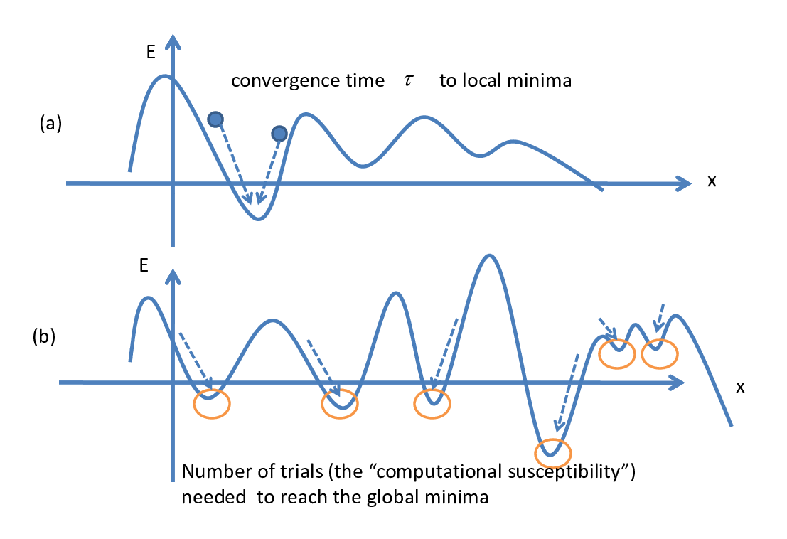
The convergence time. The convergence time is the number of the algorithm steps needed to find the local minimum following a greedy algorithm. As just noted above, a schematic plot explaining the physical meaning of the convergence time is shown in Fig. 2.
The complexity. The complexity customarily denoted as , can be derived from the number of states with energy . Specifically, , [19] where the energy density . In this work, we will numerically determine the onset of the high complexity (which probes the number of local minima) without any prior assumptions or approximations by directly computing the “computational susceptibility” ([10]) that we will briefly define next.
The “computational susceptibility”.
A “computational susceptibility” monitoring the onset of high complexity can be defined as:
| (7) |
That is, is the increase in the normalized multure information as the number of trials (number of initial starting points in the energy landscape) is increased. Physically, we ask how many different initial starting points in the energy landscape (i.e., how many different initial “trials”) are required to achieve a certain desired threshold accuracy as measured by information theory measures.


VI Noise tests
Similar to [34], we will use a “noise test” benchmark as a workhorse to study phase transitions in random graphs [9].
We define the system “noise” in community detection problem as edges that connect a given node to communities other than its original community assignment (“inter-community” edges). In general [9], we cannot initially distinguish between edges contributing to noise and those constituting edges within communities of the best partition(s).
Specifically, for each constructed benchmark graph, we start with nodes divided into communities with a power law size distribution (with the exponent determining the community size distribution [34] set equal to , i.e., the community size scales as with ). We connect all “intra-community” edges at a high average edge density . This, when we have decoupled clusters with no inter-community links. We then add random “inter-community” edges (“noise”) at a density of . Specifically, is defined as the ratio of the existing intra-community edges over the maximal intra-community edges, and is defined as the ratio of the existing “inter-community” edges over the maximal inter-community edges. If we denote the average external degree for each node by (i.e., the average number of links between a given node to nodes in communities other than its own) and the average internal degree by (i.e., the average number of links to nodes in the same community- with the average coordination number), then we define [9]
| (8) |
and
| (9) |
In the above, as throughout, denotes the number of nodes in community .
When the noise is low (i.e., when is small), all the communities are well defined. As more and more external links are progressively added to the system ( increases), the communities become harder and harder to detect. In some stage, when the external link density is efficiently high, the system cannot be detected. As alluded to earlier, we investigate the phase transition from the “solvable” to “unsolvable” at both the low and high temperature with the use of the heat bath algorithm (“HBA” in Appendix B) in the following section.
VII Spin glass type transitions
VII.1 Results for information theory correlation and thermodynamic quantities
With all of the preliminaries now in place, we now report our findings. The upshot of the results to be presented is evidence for the existence of two spin glass type transitions in general random graphs. Evidence for these transition is afforded by changes in the accuracy of the solution obtained by the “APM” in Eq. (1) when noise is introduced. This is shown in Fig. 3. The variation of information between the test system result and the solution displays a phase transition as the noise increases. A transition is also manifest in the sudden jump of . The variation of information remains zero (indicating, essentially, perfect solutions) up to a threshold value of the noise where a very sharp transition is seen. We compared this transition to similar transitions that we detected via more standard, methods. These are labeled, in Fig. 3, by “Q-opt SA” (maximization of modularity (Q), set by a comparison to a null model, [8] as solved by simulated annealing (SA)) and “RBPM” (the Potts model of [11] wherein the parameters in the Hamiltonian are also defined by a null model). As seen, our “APM” of Eq. (1) (which is free [10] of the so-called “resolution limit” [1, 35] that appears in systems with null models) can be used to examine graphs with high levels of noise [9]. By comparison to other models compared to null models, the APM exhibits a sharper transition as the number of nodes is increased [10].
VII.2 General features of the phase diagram as ascertained by numerical data
As is evident in Fig. 4, there are three different phases. We denote these phases by the qualifiers of (i)“easy”, (ii)“hard”, and (iii)“unsolvable”. These three phases are the analogs of the three phases (i)“SAT”, (ii)“hard”, (iii)“unSAT” in the k-SAT problem [19]. In later discussions, we elaborate on their possible physical significance of these phases in disparate arenas such as that of supercooled liquids. In what follows, we first present our results. We first discuss the zero temperature case () and then explore the physics at .


VII.2.1
In Fig. 4, the low noise region () is seen to be in the “easy” phase. In this phase, the accuracy (), entropy (), and the computational susceptibility () are constant. Within this regime, the algorithm is able to correctly distribute nodes into their correct communities. We test several systems with different system size and number of communities , and in Appendix E, we plot the first transition point in terms of and .
As the noise is further increased beyond a threshold value of , the system enters the “hard” phase. The existence of the “hard” phase is reflected by the rapid growth (decrease) in the entropy and computational susceptibility (accuracy) curves. Even though, we can increase the number of trials in order to improve the accuracy of our solutions (as seen in panel (c) of Fig. 4), it is, nevertheless, still hard to obtain exact solutions.
As the noise is yet further increased and exceeds a second threshold value (), the system undergoes another phase transition from the “hard” phase to an “unsolvable” phase. This “unsolvable” region is reflected, amongst other things, by the collapse of all of the curves in each panel of Fig. 4. In this regime, it is impossible to solve the system correctly without infinite time in the third region.
VII.2.2
A more detailed, higher dimensional perspective, that includes the effects of temperature is provided in Fig. 5. In this figure, summarizing our results for the computational susceptibility , Shannon entropy , normalized mutual information and system energy at general finite temperatures , we plot the loci of point marking the boundaries between the different phases. The “flat” phase that lies in the middle of these panels is the “easy” phase. [Within the “easy” phase, the system is easily solvable and the planted communities are perfectly detected.] This “easy” phase is separated by “ridges” of high computational susceptibility (marking the ”hard” regions) from the “unsolvable” phases. As expected, the computational susceptibility/energy/entropy/ exhibit a precipitous jump as the noise exceeds some threshold value . A low temperature hard phase appear for noise levels . We can determine the boundaries of the“hard” phase, whenever it generally exists, by seeing for which values of and there is a rapid increase of and . An additional high temperature bump in the computational complexity and appears for noise levels . In this phase, the minimization of Eq. (1) is non-trivial. At yet higher temperatures/noise levels, it is generally impossible to solve the system. Thus, the two loci of “ridges” in the computational complexity (i.e., or ) delineate the “hard” phases. To emphasize the appearance of this ridges and their manifestation in all measured quantities, a guide to the eye is drawn. Within the low temperature hard phase (), the system becomes trapped in the local energy minima (panel (a) of Fig. (6)). At low temperatures, we find from the exact and extensive numerical calculations (as shown in panel (d) in Fig. 4), a very dramatic increase in complexity just at the transition followed by a much more gradual decrease up to . The convergence time for a local greedy algorithm (such as ours shown in (c) of Fig. 4) does not correlate with the complexity as the system. This is so as the system can easily converge to a wrong local metastable minimum (while the number of such minima is given by the complexity).
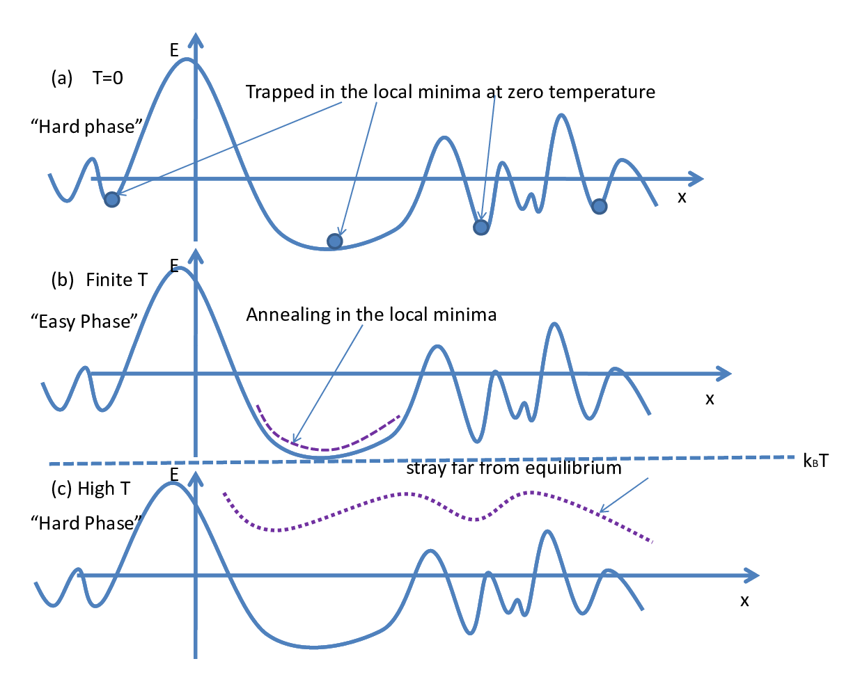


In Fig. 6, we provide caricatures of the underlying physics in these phases and the low temperature/low noise transitions. At low temperatures, for noise slightly above (at zero temperature), the system becomes quenched in metastable local minima at low temperatures. This is schematically illustrated in panel (a). As the temperature is increased, the system may, as depicted in panel (b) of Fig. 6, veer towards its global minimum by annealing. Physically, a similar mechanism is at work in many frustrated physical system where it goes under the name of “order by disorder” . In such cases, by virtue of entropic fluctuations, quenching is thwarted and the system may probe low lying states and indeed order [36, 37, 38, 39]. Thus, the energy and computational susceptibility may remain constant (there is only one global energy minimum, i.e., one state or a finite set of such states). However, it does take progressively more time to locate the global minimum state ((c) in Fig. 4). As the noise is further increased, the system is still ergodic. However, it takes a very long time to find the lowest energy state. On finite time scales, the system stays in the vicinity of local minima thus yielding a higher observed energy. Only on sufficiently long time scales does the system veer towards its global minimum (or minima). Within this “hard” region, there are many metastable states. This leads to a significant increase in the complexity as is made evident by the rapid growth of the computational susceptibility of Eq. (7). The large computational complexity marks the initial rapid climb of the complexity.
We now return to the results of Fig. 5 at yet higher temperatures and values of the noise . The high temperature “ridge” in Fig. 5 () corresponds to the system being far away from the minimum energy state. As we remarked earlier, this delineates yet another “hard” phase. According to the above explanation and the corresponding caricature of Fig. 6, increasing the running time and/or number of trials should help increase the accuracy of the solution in this region (the peak area of the computational susceptibility). Beyond this region, at higher temperatures, the system is unsolvable. This corresponds to panel (c) in Fig. (6).
At low temperatures and high noise, due to the proliferation of metastable states, (i) the convergence time (as seen in panel (c) of Fig. (4)) can be low while (ii) the increase in accuracy by performing more and more trials is, essentially, nil [as seen by the low value of in panel (d) of Fig. 5]. Similar conclusions can be arrived at finite temperatures by examining constant slices of .


We now examine, in further detail, several aspects of these transitions at . The (zero-temperature) normalized mutual information is displayed in Fig. 7. As evident from the figure, starts to drop below its maximal value of (which indicates perfect agreement with the optimal solution) when (i.e., at the very same value of the noise where the relaxation time is maximal and the complexity increases) and levels off at a higher value of the noise (coincident with the transition value as ascertained from the energy, entropy and complexity in Fig. 4). Amongst other collapses that we observed, systems with differing number of communities q all collapse onto at .
Before we turn to a more detailed analysis of spin-glass character of the transitions, we make one remark. A possible concern is that we did not examine transitions the optimal value of . Indeed, the central thesis of [9] was that there are optimal values of that signify the natural scales in the system. In general, transitions as a function of correspond to transitions in structure that appear as the system is examined on larger and larger scales as we have examined in detail in earlier works [9, 28, 29, 27]. To ascertain the changes that occur in the random systems that we investigated in this article for a broad spectrum of different values of (i.e., containing general ), we re-investigated these systems with values within the range . The “best ” values of are ascertained by maxima of the normalized mutual information [10]. In Fig. 8, we display as the function of the noise for both the fixed and the optimal determined by the multiresolution algorithm. The first transition point is the same in both cases, and the two curves start to separate around the second transition point . This indicates that, as it so happens to be in this case, is the best value of resolution parameter for noise levels below in this example system () at zero temperature.


VII.3 Numerical validation of the spin glass character of the two transitions
The proliferation of metastable states thwarts equilibration. A specific facet of this is detailed in Appendix F wherein, by energy measurements, the lack of equilibration at short times is evident. As is well appreciated, this absence of equilibration due to multiple metastable states may lead to spin-glass-like (as well as structural glass like) properties. Amongst other traits, these include memory effects previously studied for other systems [40, 41]. When a spin glass is cooled down, a memory of the cooling process is imprinted in the spin structure, and this process will be reproduced if one heats the system up.
We conduct a similar computational “experiment”. We immerse our system (with a fixed value of the noise ) in a heat bath. We then lower the heat bath temperature by small increments at consecutive time steps . (Each time step corresponds to a single iteration through all nodes according to the minimization algorithm of [9, 10].) In this case, we set . After attaining a steady-state solution, we then reverse the process and increase after each step via . In Fig. 9, we plot the long time system energy as a function of during this process. The energy curve as decreases follows a different path than when increases which strongly implies a hysteresis-like effect. This memory effect as the temperature is cycled between high and low reinforces the similarity between the community detection and a spin glass system.
The behavior of the energy displayed in Fig. 9 suggests the same three regions that we ascertained earlier: (i) When the two curves overlap at low temperatures (i.e., ), the system is in its “frozen phase”. (ii) When the two curves separate in a medium temperature range (i.e., ), the system is in a“spin-glass” phase. (iii) At yet higher temperature (), the two curves overlap once again. This marks the onset of the “disordered” high temperature regime.


As illustrated in Figs.(4,5) (and as will be further discussed in Figs. (11,12)), the hard phases at both low and high temperatures do not extend over all temperatures. Rather, as we have emphasized above, the hard phases only appear in the “complexity” ridges as shown in panel (a) of Fig. 5. However, in Fig. 9, the hysteresis occurs in the temperature range . This range is considerably larger than that of the hard phases. To understand this, we remark on the “experimental” differences between the results displayed in Fig. 5 and those in Fig. 9. In constructing the 3D plot of the “complexity” (panel (a)) in Fig. 5, we apply the “HBA” at each temperature. The systems at different temperatures are independent of one another. That is, each system is solved afresh from the symmetric initial state. In the hysteresis loop in Fig. 9 on, e.g., the decreasing temperature curve, a system at higher temperature provides the initial state for a lower temperature system. Thus, in this case, the systems at different temperatures are not independent but rather serve as “seed” states for one another.
Aspects of the memory effect are evidently not limited to those of, e.g., Fig. 9. For instance, if we incorporate the effects of increasing and decreasing noise to the same system [43] instead of temperature, the accuracy of the solution also forms a hysteresis loop at low temperature (see Appendix C). Similar to a real spin glass system, the magnitude of this effect also decreases as the temperature increases and finally disappears beyond a threshold temperature.
A general quantitative measure of the memory, the two-time autocorrelation function between the system at times and time ,
| (10) |
can be used to explore the spin-glass-like behavior. The upshot of the below discussion is that the autocorrelation function data only within the hard phases (both at low and at high temperatures- coincident, as emphasized earlier, with the “ridges” in Fig. (5)) adheres to a spin-glass type collapse. This affirms, once again, the spin glass character of the transitions.
If we apply the HBA starting from different initial configurations at low temperature (as elaborated on in Appendix D), all of the auto-correlation curves with different initializations separate from each other even up to times [in units of the iteration through all nodes according to the algorithm of [9, 10]] as large as (Fig. 10). This indicates that disparate sorts of randomness can, generally, lead to different results. As the temperature is increased, all of the curves ultimately collapse onto one another. The temperature at which the different initial configurations overlap indicates when the respective systems start losing memory of their initial configurations directly relates to the transition temperature in the hysteresis loop for the same system. This further establishes the existence of spin glass transition in the community detection problem.
We use the HBA starting from a symmetric initial state and calculate the autocorrelation in Eq. (10) for different waiting times and temperatures . We further found that each auto-correlation curve corresponding to longer waiting time lies above those with shorter waiting times, and all the curves (with different waiting times) are non-zero for a long period of simulation time indicating a memory effect. Moreover, we can predict the long time behavior of by fitting the curves using a commonly-used equation in Fig. (11, 12), for more details, see [44, 45].
Towards this end, we set
| (11) |
and
| (12) |
In the above equations, , and are parameters that need to be optimized in order to ascertain whether a generic spin glass type collapse occurs [44, 45]. In searching for a collapse of the data points at different waiting times , we use as a vertical-axis and as a horizontal-axis. As seen in Figs. (11, 12), a collapse indeed occurs over 4 decades in values of in both the high and low temperature hard phases.
We discuss several features of this collapse and its coincidence with the hard phase below. Fig. 11 corresponds to the low temperature hard phase and Fig. 12 corresponds to the high temperature hard phase [see, e.g., the 3D computational susceptibility plot in Fig. 5]. As seen in Figs.(11, 12), both the high and low temperature cases, the autocorrelation functions with different waiting times exhibit spin-glass collapse when the value of lies within the “ridge” area of the hard phases. This collapse wanes when veers towards the “foot” of the complexity ridge just at the onset of the hard phase. The collapse ultimately becomes non-existent when is further away from the “ridge” area. The regime where the correlation functions satisfy the spin-glass collapse is consistent with the parameters corresponding to the hard phase (or “ridge” in the 3D computational susceptibility plot of Fig. (5)). Putting all of the pieces together, we see from our scaling and collapse in Figs. (11, 12), that both high and low temperature transitions of the spin-glass type.
In the random graphs, we reported on spin-glass type transitions. Although trivial, for completeness, we should however note that a graph can, obviously, also be very regular. A prototypical example is that of the two-dimensional square lattice [42]. For such regular unfrustrated lattice systems, the Potts model of Eq. (1) becomes the “standard” Potts model of lattice systems. In these instances, we generally have single first or second order transitions instead of spin-glass type transitions. We briefly elaborate on this point. Simple regular lattices are a particular realization of a graph (one with the fixed coordination and translational symmetry). As is well known, on, e.g., the square lattice, the Potts model, which we use throughout, exhibits as a function of the temperature , two phases with an intervening critical point for small (); for larger (), a first order transition appears. Thus, particular realizations of our hamiltonian for these graphs display (usual) critical points and first order phase transitions. For more generic random graphs with high coordination, the system displays (as we showed above and will further elaborate on), spin-glass type transitions appear along with intervening hard phases.
We further reiterate an earlier remark and note that in systems with well defined structures on multiple scales, additional transitions may appear as the resolution parameter of Eq. (1) is varied. In earlier works, we reported on these transitions and further employed these in the analysis of disparate systems [9, 28, 29, 27].
VII.4 General discussion
In this subsection, we detail general considerations directly related to the spin-glass Potts analysis thus far. In the next section, we will further discuss dynamics which further relates to aspects that we detail herein. This subsection is different from others in that here (and only in this subsection), we present a general discussion and some speculations and not present data.
VII.4.1 Theoretical Expectations from NP-completeness
In [46], it was shown that maximizing modularity (an earlier alluded to prominent approach for the community detection problem [1, 8, 22]) is NP-complete. Thus, as all NP complete problems may (by their very definition) be mapped onto one another, maximizing modularity on the most general graphs must span the three phases (solvable and unsolvable with the further division of the solvable problems into the “easily solvable phase” and the “hard phase”) that appear, e.g., in k-SAT problem [19] which is known to be NP-complete [47]. Similarly, if other approaches to community detection are, ultimately, equally hard as maximizing modularity, then all of these approaches may in general display three phases. It may be, as in the k-SAT problem, that for simple problems, we have only an “easy phase” and an “unsolvable” (or “unSAT”) phase. This does indeed occur for some graphs. In general, though, we find the three different phases (as expected) that we reported on in this work.
VII.4.2 Physical content of the transition in many body systems
Approximate decoupling
We briefly speculate, in this subsection alone, on potential physical consequences of the phase transition that we find in the community detection problem. As elaborated on in [28, 29] a general many body system with two particle interactions may be regarded as a network with edge weights determined by the interactions. In the easy phase in the extreme limit of , the system is essentially that of disjoint non-interacting clusters. This point is analytically connected to any other point in the easy phase. More generally, The Potts model Hamiltonian Eq. (1) can be written as: . Thus, the partition function becomes:
| (13) |
In Eq. (13), is the partition function as computed with the Hamiltonian of the entire system for the particles in community k, and denote partitions of the system.
A similar form was proposed for many body systems in [28] when partitioning a general interacting system into decoupled clusters. Even though, we sum over all partitions, we may have an important subset of partitions, denoted as (each with a corresponding number of clusters equal to ), which will have in general instances, high Boltzmann weights and/or frequencies and will dominate the sum. These partitions will, correspondingly, have a significant lower free energy relative to other partitions. In such cases, the partition function can be approximated as
| (14) |
Eq. (14) is exact in the limit of where denotes the ground-state(s) of our Potts type Hamiltonian. If is small (in particular if ), then there will generally exist a small number of sharply defined ground-states pertaining to partitions into completely disconnected communities. This general trend of dominant subsets may persist within the easily solvable phase.
The possible upshot of this discussion is that we might, in easy phases,
approximate many body interacting systems (such as supercooled liquids
that we will briefly discuss next) as effectively composed of disjoint
non-interacting clusters. This picture may badly break down
once transition lines between the easy phase and the
hard or unsolvable phases are traversed.
Possible relation to structural glasses and other complex physical systems
Glasses (according to the theories such as the random first order transition theory of glass (RFOT) in [48]) may have three phases as a function of temperature. In the intermediate phase, the system displays a large complexity (as manifest in the configurational entropy being extensive). If we replace the interacting particles in a supercooled liquid (that form a glass at low temperatures) by decoupled communities [28, 29], then the three phases found in the computational community detection problem may be manifest as three disparate phases of supercooled liquids as a function of temperature. Within RFOT, at temperatures in an intermediate region ), the system physically displays an extensive configurational entropy (which is tantamount to an extremely large complexity in the current context). This configurational entropy precipitously onsets at and gradually diminishes until it no longer becomes extensive a lower temperature () whence the system freezes into an “ideal glass” that is permanently stuck in a metastable state.
We will discuss, in Section VIII dynamical aspects that directly relate to the Potts model Hamiltonian. Insofar as additional general related aspects of the results of our community detection analysis the implication of phase boundaries, we make a brief comment. When, as discussed in [28, 29], a weighted version of Eq.(1) is used with edge weights that are set by forces then in overdamped viscuous systems (where the total force on a particle is proportional to its velocity, ), particles that experience a similar total force, will tend to move in unison. Thus, in the easy phase motion of decoupled cohesively moving particles will occur. In the unsolvable phase, the particle motion will be more complicated. In earlier work, forces were used to study community detection with, overall, similar results to the one afforded by our spin glass approach in this work [12]. When other weights are used (such as potentials, two-body correlations or other metrics), similar decoupling within the solvable phase signifies a tendency of the clusters not to be related insofar as the metric being used.
VII.4.3 Image segmentation
Recently, we investigated and invoked the features of the phase diagram in order to address the computer vision problem of detecting objects in general images [27] (including notably challenging ones). As in in this work for random graphs, by varying parameters such the temperature,the (graph) resolution parameter and physical length scales, we explored the community detection phase diagrams for image segmentation. Within the easy phase, disparate objects were clearly seen. As the system moved into the hard phase, the sharpness of the objects became more fragmented. These ultimately became very noisy in the unsolvable phase.
In summary, whenever a decomposition of an interacting many body system into nearly decoupled communities is possible (indeed, as alluded to above, such a decomposition is exact for Potts model systems wherein the exchange energy between spins in different domains is zero) then the phase transitions that we report on here for the community detection problem may carry direct physical consequences. This may afford a direct link between the phase diagrams of hard computational problems (as ascertained by physically inspired approaches) and the phase diagrams of physical systems that may be investigated via solutions to these related computational problems. It is important to note that the direct relation between complexity and glassiness is not simple as some problems that may be investigated by sub-optimal algorithms (such as physical stochastic systems) may appear to have a “hard phase” while if investigated by a more efficient algorithm do not have a “hard phase” [49]. Nevertheless, it may well be possible that the decomposition of physical systems into simple elements will no longer be simple at the onset into complex states such as those of supercooled liquids. Indeed, in recent work, we applied the community detection ideas to general many body systems (including glasses) in order to flesh out prospective important structures on all scales [28, 29, 27].
VIII Dynamical Aspects
In the following, we also study the related dynamical transition. Dynamic approaches to community detection have been suggested earlier [12, 50]. To describe the dynamical process, we need to calculate the trajectory (of community memberships) for each node as a function of time. Specifically, we use the correspondence between the -state Potts model and a clock-type model in dimensions. We replace the Kronecker delta in Eq. (1) by a product where and are the vertices of a regular -dimensional simplex. On such simplifies (e.g., an equilateral triangle (), tetrahedron (), …), . Thus, as is well known, we can cast the Hamiltonian of Eq. (1) into the form where is the interaction weight. If we insert an external field into this simplified Hamiltonian, then it becomes
| (15) |
In what follows, we will first outline a very simple new general method for relating a general statistical mechanics system (such as the particular Potts model under consideration) and a dynamical system from classical mechanics. Although, this method will be specifically invoked to the Potts model, all of its steps can be replicated for other systems as well. We will then proceed to show the results of our numerical analysis. The final result of our analysis is that the spin glass transitions relate to transitions to chaos in the dynamics of the continuous mechanical system.
VIII.1 Relating discrete Hamiltonians to continuous dynamics
We will in this subsection illustrate how it is possible to relate the discrete Potts model Hamiltonian of Eq. (1) [and its clock model variant of Eq. (15)] to mechanical system with continuous dynamics. Many possible similar variants of the method outlined below are possible. Although our present aim is to investigate the Potts model Hamiltonians, as noted above, our method can be applied mutatis mutandis to general discrete Hamiltonians. A benefit of this mapping is that it bridges chaos in the more standard mechanical sense to that reported in spin glass systems.
Starting with Eq.(15), we perform a Hubbard-Stratonovich transformation via non-compact auxiliary fields to arrive at the effective Hamiltonian (or, more precisely, free energy)
| (16) | |||||
where is the partition function.
The dynamical equation for a node moving under the effective field is, for a damped system, given by
| (17) | |||||
We initialize the auxiliary field to be some constant vector close to . We can solve this dynamical relation to obtain the non-compact auxiliary field as a function of time [51].
We can obtain the expression for nodes trajectories in terms of time by taking the derivative of the partition function ’s [Eq. (16)] with respect to the source , i.e.,
| (18) | |||||


VIII.2 Numerical results for the continuous dynamical analog
Eq. (17) describes overdamped (or Aristotelian) dynamics. It is, of course, possible to also define the system in such a way that it evolves according to Newton’s equation. In overdamped systems, the energy of the system goes down with time and thus the system veers towards a local (or global) energy minimum. The system exhibits no dynamics once it gets stuck in a local (global) minimum of the energy. For the shown system in Fig. 13 , in the absence of perturbing fields, at low noise within the solvable region the system, the node coordinates quickly collapse to the origin. Conversely, at high values of the noise (i.e., large ) the node coordinates do not converge (and indeed, as we elaborate on below, the system is not solvable). As detailed in Appendix G, we further applied weak perturbing fields and found that they can indeed veer the system, at low noise, towards the correct solutions.
The system shown in Fig. 13 contains only nodes with communities at a temperature . Prior to investigating this system using the dynamical approach outlined above, we first examined this system also using the entropy/energy/computational susceptibility measures discussed in this article and found that, in this system, there is no hard phase. Rather, there is a direct transition (or, more precisely, crossover in this small system) from an easy solvable phase for to a disordered unsolvable system for . The result of our dynamic analysis following Eq.(27), demonstrates the existence of a phase transition (or crossover for this finite system) at precisely the same values of found by the analysis of the thermodynamic quantities associated with the Potts model for this small system. In this case, the dynamics of the nodes illustrate that when exceeds , the system exhibits a transition from a stable system () to one which is chaotic (). Our dynamic approach to the community detection transition may generally bridge such transitions in system dynamics to thermodynamic phase transitions.
We illustrated via our dynamic approach, how ergodic behavior can arise depending on (and, similarly, also on temperature). This relates to “chaotic” behavior reflecting the sensitivity to the temperature and in our case other parameters (such as ) that define the computational problem in spin-glasses [52, 53, 54] to real chaotic behavior of a dynamical system. Further, in our spin-glass approach, Fig. 15 illustrates that auto-correlation functions corresponding to different initial conditions (or randomness) remain different up to long times. This sensitive dependence on the initial conditions is the hallmark of chaotic systems. Although, we have not observed such an intermediate hard phase for the small system that we investigated using this dynamic approach, we speculate the above dynamic transition from more stable orbits to “chaos” may, for larger systems, exhibit also indeed an intermediate region corresponding ( for low or also for higher ) where more and more branching points may appear (or period doubling, etc.) as the system transitions into chaos. Ideas from KAM analysis may, hopefully, be invoked in more sophisticated treatments.
IX Conclusions
We reported on disparate high and low temperature spin glass type phase transitions in the community detection problem and, by extension, rather general disordered Potts spin systems. Our investigation involved several complementary approaches and was not confined to systems with a small number of Potts spin flavors or communities. In the community detection setting, similar to other computational problems, phase transitions occur between a solvable and unsolvable region. The solvable region may further split into an “easy” and a “hard” region. We illustrated how thermal “order out of disorder” may come into play in these systems and provided ample evidence of the spin-glass character of the transitions that occur. Amongst other results, we found that different sorts of randomness can lead to different behaviors, e.g., “chaos”. We introduce a general correspondence between discrete spin systems and mechanical systems with continuous dynamics. With the aid of this mapping, we illustrated that spin glass type transitions in the disordered system correspond to transitions to chaos in the mechanical system. The mapping that we use to relate the thermodynamics to the dynamics suggests how chaotic-type behavior in thermodynamical system can indeed naturally arise in hard-computational problem and spin-glasses. We further briefly speculate on possible physical consequences (such as supercooled liquids and glasses) of the transitions that we find here. Recently, we indeed employed the transitions that we found here in the analysis of such complex physical systems [28, 29] as well as image segmentation [27].
Acknowledgments. This work was supported by NSF grant DMR-1106293 (ZN). We also wish to thank S. Chakrabarty, R. Darst, P. Johnson, B. Leonard, A. Middleton, M. E. J. Newman, D. Reichman, V. Tran, and L. Zdeborova for discussions and ongoing work.
Note added in Proof: Some time after the initial appearance of the current work [55] and earlier reports of particular aspects of a phase transition (Appendix E of [9] and Appendix B of [10]), the authors of Ref. [56] investigated phase transitions in the community detection problem on sparse graphs of small and reached similar conclusions as we have for general graphs with larger values.
Appendix A: Theory analysis of the community detection problem
In this appendix, we follow the description of cavity method in [32] and merely generalize it to all graphs (general and unequal size communities). The uninitiated reader is encouraged to peruse [32] in order to familiarize him/herself with basic the cavity method (and the notations) used that we expand on below. The brief introduction below is not self-contained.
Within the cavity approach, each node passes a message along edges. A message from node to is a -dimensional vector of zeros and ones. Node takes the messages from all the other nodes connected to and sums them. Then the cavity field defined as is obtained through the above process. Finally, node converts this cavity field into a message to by picking and setting the maximal components in to one and the rest to zero. The probability distribution of messages being sent in the system is denoted as . The superscript denotes a possible dependence of this distribution on the index of the pre-defined cluster to which the sending node belongs.
To be consistent with the notations in [32], in what follows in this appendix (and only in this appendix), we will employ the same definition for and as that of [32]. For a fixed cluster , is the conditional probability that a link starting with a node in also ends in . Given two (different) clusters and , denotes the conditional probability that a link starting with a node in would end in . It follows directly from these definitions that,
| (19) |
In particular, when , there are only two clusters/states which , and we have
Following the same calculation process in [32], we also test the phase transition of community detection in a random Bethe lattice with exact degree . But there is an essential difference that our Hamiltonian does not have the constraint of equal-size clusters, which means we do not have the symmetric condition for the order parameter , where, denotes the “correct” component, and denotes the number label of a“wrong” component. In our case, now can not be necessarily written as ; we now write this as .
We first discuss the case of and then proceed to its generalization.
In systems with two clusters (), the are two (Potts) spin states. We will denote these herein as and (once again, we do so to be consistent with the notations in [32], in particular Eqs. (6.60)-(6.63) therein). In this case, there are different “order parameters”. We will denote these as , , , , and .
In the following, we present the expressions for , and . The expressions for , and have an identical form with a permutation of the superscripts .
| (20) | |||||
| (21) | |||||
| (22) | |||||
These consist a quadratic system of equations with variables. This system of equations is numerically solvable. The solutions are continuous with respect to coefficients , . The new equations of Eqs. (20,21,22) form a generalization of the system studied in [32].
The above procedure can also be easily generalized to system with components leading to more terms on the righthand side of Eqs. (20,21,22). In general, we can define an abstract function :
then for any
and , we have the equation
| (23) | |||||
In the above equation (Eq. (23)), denotes the q-dimensional incoming message composed of and s. We introduce (,) to be any pair of vectors that “sum up to” a given vector , in the sense of . We are able to numerically evaluate the order parameter as a function of .
From this, we can obtain the phase boundaries of the solvable region. Furthermore, to test whether our simulation result matches the theory, we perform the same accuracy test using our greedy algorithm on ER graphs with and four equal-sized clusters. Our result of Fig. 12 in [10] in Appendix A is consistent with the cavity inspired result of Fig. 6.7 in [32]. In both plots of the percentage of correctly identified nodes in terms of , the critical value of and for the accuracy drops are the same if we transfer into via the relation (for the graphs considered therein with an average total coordination number per node of ). In, e.g., Fig. 6.7 of Ref. [32], the threshold value of is given by . In Fig. 12 of [10], the critical obtained by our greedy algorithm is , which corresponds to .
Appendix B: Heat Bath Algorithm
We extend the zero-temperature (greedy) algorithm of [9, 10] to finite temperature via a heat bath algorithm. This algorithm allows each node to become a member of one community with probability set by a thermal distribution [11]. The probability is
| (24) |
Here is the change of energy for moving this node from cluster to cluster , and runs through all connected clusters (neighbors) of this node (including the case that , i.e., this node remains in cluster ; and the case that is a newly added cluster, i.e., this node becomes a new sole-node cluster).
The steps of our heat bath algorithm are as follows:
(1) Initialize the system. Symmetrically initialize the system by assigning each node to its own community. (i.e., ). If the number of communities is constrained to some value , we instead randomly initialize the system into communities.
(2) Find the best cluster for node . Sequentially “pick up” each node and scan its neighbor list (include its current cluster and the newly added cluster). Calculate the energy change as if it were moved to each connected cluster. Then calculate the probability for an arbitrary node in cluster to be moved to a connected cluster using Eq. (24). Then we use all the probabilities for different j’s to determine which cluster to be moved to; i.e., generate a random number between and , then determine which probability range the random number is in, and move the node from cluster to the selected cluster .
(3) Repeat step 2 for all nodes in the system. A node is frozen for the current iteration once it has been considered for a move.
(4) Merge clusters. Allow for the merger of two communities together based on the merge probability. Towards this end, we calculate the energy change as if the current community is merged with its neighbors. We then use Eq. (24) to calculate merge probabilities.
(5) Repeat the above two steps. Repeat step to until the maximum number of iterations is reached.
(6) Repeat all the above steps for s trials. Repeat step - for trials and select the lowest energy result as the best solution. Each trial randomly permutes the order of nodes in the symmetric initial state.
The new algorithm is similar to the earlier greedy algorithm [9, 10] except for steps (2) and (4). The nodes are moved based on a random process. Thus, the outcome may be sometimes sensitive to the initial random seed state. As noted within the main text, when the system is within the easy phase, all seeds lead to the same final outcome. However, when the system is within the hard phase changing the random seed may significantly alter the final result. In such a case, different initial conditions enable the system to get stuck in different local minima (each corresponding to a different partition of the system into disparate communities). This is why we repeat the procedures for trials (usually is set to be ). The additional trials sample different solutions evenly with the symmetric initialization, and it will reduce the dependence on initial conditions. In the unsolvable phase, for any finite number of trials , the quality of the solutions does not visibly change.
We should note that the new “heat bath algorithm” that we introduced above is different from the commonly used “simulated annealing algorithm”. (The latter is a generalization of the “Metropolis Monte Carlo” procedure (MMC) [57])).
Within the conventional MMC procedure, the probability for an arbitrary node to be moved in cluster to a connected cluster is given by . This implies that a node in community will (with certainty) be moved to cluster if the energy change is negative. Such an algorithm precludes for a lower energy move (if such a later move will be found later on). By contrast, within our “heat bath algorithm”, nodes are not immediately moved to the first tried clusters if the energy change is negative. We compute the probabilities of connected clusters. Obviously, the cluster with the largest energy decrease would have the largest probability to be the “candidate of absorption” for node . Thus, in contrasting the commonly used MMC procedure and our HBA, it seems be easier to get to the lowest energy state of the studied system within our algorithm. Our procedure allows nodes to explore more energy states in each step and better equilibrate.
Appendix C: Memory effect in versus noise plot


In the main text of the article, we provided an example of a hysteresis by decreasing and then increasing the temperature of the system (see Fig. 9). However, examples are not limited to this particular cycle [43]. Other ways to see the memory effect include varying the noise level. This appendix is devoted to the study of the hysteresis curves in such a case. That is, in this appendix we consider the effect of adding external edges between disparate communities (i.e., increasing ) and then removing these edges (i.e., decreasing ). We examine the accuracy of solutions as a function of noise and see whether the two curves coincide. The non-coincidence between the two processes will exhibit exactly the same memory effect that we earlier reported on by varying the temperature.
Fig. 14 shows the results of the above experiments at three temperatures: , and . In the systems, the curves with increasing and decreasing form hysteresis loops. The hysteresis loop in temperature in panel (b) is less significant than its counterpart for at in panel (a). Upon further increase of the temperature, the hysteresis disappears (as shown in panel (c)).
The plots in Fig. 14 have already exhibited decreasing memory effects as the temperature increased. Thus, there must exist a temperature beyond which the effect disappears. We investigated the plots at temperatures (not shown here). The hysteresis loop disappeared at about in line with our other reported results including the disappearance (at of memory of initial conditions to which we turn to next.
Appendix D: Memory effect in correlation functions with different initial conditions


In this appendix, we report on the autocorrelation functions (Eq. (10)) for three different types of initial configurations. The conclusion of this appendix is that the system may be sensitive to initial conditions. The three initializations are denoted as symmetric, random and power law distribution.
“Symmetric” initialization alludes to an initialization wherein each node forms its own community, so there are communities in the beginning (as in step (1) of the algorithm outlined in Appendix B).
“Random” refers to randomly filling in communities with nodes, where is a random number generated between and .
In the “Power law distribution” nodes are partitioned into different communities whose size adheres to a power law distribution (Prob ) with a negative exponent . In the cases displayed, we set .
The maximal community size in the true solution is set to be and the minimal community size is .
Fig. 15 vividly illustrates that all the curves with different initializations separate, at low temperatures, from each other even up to times of size . The curve with symmetric initialization lies on the bottom in panel (a). However, as temperature increases, all of the curves veer towards each another. The symmetric curve moves form the bottom to the top at a temperature as shown in panel (b). As temperature increases furthermore (), all of the curves overlap in panel (c).
At a temperature of , systems with different initial configurations start to overlapping. Beyond this temperature, there is no remaining memory of the initial conditions. Furthermore, the relative position of the curves become different, which is another indication for the lose of memory. The spin temperature at which we found the hysteresis loop to disappear in Fig. 14, , nearly coincides with the temperature found here.
In Fig. 15, the relative positions for the “random” and “power law distribution” do not persist: their positions change irregularly as temperature varies. This indicates that these two are similar to each other– there is no essential difference between them. However, the curve of symmetric initialization lies below the other two until the temperature rises up to , which happens in all the waiting times that we tested (, and (not shown here)). This suggests that the symmetric initialization differs, in an essential way, from the other two initializations.
Appendix E: Finite size effects
In this appendix, we examine the zero temperature transition at for systems with different system sizes and community numbers .


In Fig. 16, we display, at zero temperature, the first phase transition point (we remind the reader that this nose levels marks the first transition point encountered as is increased) as a function of the community number (panel (a)) and the system size (panel (b)). From the numerical results that we obtained, we find that relates linearly . As seen in Fig. 16 panel (a), the value of the first phase transition point in each curve approaches zero as increases. This is consistent with what is expected: for a fixed system size, increasing the number of spin flavors introduces a multitude of possible states and the system becomes progressively disordered.
This may also be made analytical via a type expansion wherein the partition of the Potts model is expanded in terms of correlations (of having two () and then three etc.) connected spins be of the same flavor. The resulting terms in such an expansion illustrate that increasing emulates (not too surprisingly increasing the temperature ). For a system at large (i.e., a system in thermodynamic limit), increasing renders the system progressively less ordered. Thus, in situations such as that of an increasing number of communities that scales linearly with the system size (such that the average community size remains constant), the transitions become less well defined as . In the fitting form below of Eq.(25), the saturation of the system phase diagram for large and the relatively quick drop in the sensitivity of our results to finite size effects becomes apparent.
On the other hand, from panel (b) in Fig. 16, for a fixed , when is small, first increases with a very steep slow and thence increases very slowly with a nearly plateau behavior. We can interpret these data by the function , where is a constant for each (e.g., for , and ). Combining both panels, we can present in the examined range as a two-variable function and ,
| (25) |
Thus, as alluded to above, finite size effects drop and features of the system phase diagram (as evidenced by above) saturate for large . Thus, in considering limits such while holding the average community size fixed, we essentially increase for a system in the thermodynamic limit.
Appendix F: Equilibration times
In equilibrium, the energy is (of course) constant. The system energy is set by its temperature. In this appendix we investigate, at different temperatures, the evolution of the system from an initial high energy states. In the particular results that we provide below, the energy of the disparate systems at low temperatures would, at short times, naively seem to violate thermodynamic expectations. Systems with lower temperature can have higher energies than those at higher temperature. The origin of this and similar effects is that significant time may be required to achieve thermodynamic equilibrium. Within the low temperature unsolvable phase the system is out of equilibrium. In the hard phase, equilibrium is achieved yet it requires long times.


We now present our results. We set the system size (number of nodes) to be with communities and a value of the noise given by . As such, with this value of which is larger than the threshold value of for this system, the system is in the “hard” phase. We examine the system evolution with the algorithm time steps in Fig. 17. In this plot, the system has a “crossover” at about . Prior to that time, the energy always decreases as increases. This reflects the fact times below are not long enough for the system to equilibrate. After that, except for the cases of , or , the energy turns to increase as increases. Thus, constitutes sufficient time for equilibration except a few systems at very low temperature (that require yet longer times). This “crossover” property for system is a sign of the restoration of equilibrium at sufficiently long times.
All the curves show a decrease of the energy with time until a plateau in reached. When time is not sufficiently long, the system is not ergodic and out of equilibrium. As seen in Fig. 17, times are required for lowest temperature systems (e.g., , ) to equilibrate.
Appendix G: Nodes’ trajectory after applying the perturbation field
As mentioned earlier in the text, effective fields may direct the continuous dynamical system of Section (VIII) towards correct non-trivial solutions. In this brief appendix, we outline how this is achieved and provide some results.
The dynamical equation for a node moving under the effective field is
| (26) |
Similarly to Section (VIII) yet now with general applied fields, we have
| (27) |
As shown in Fig. 18, if we choose the perturbation field to favor a preset community membership for each node, i.e., let , where is a small constant value, then within the solvable phase the nodes will be biased towards the corresponding particular partition of the system.
References
- [1] S. Fortunato, Community detection in graphs, Physics Reports 486, 75-174 (2010).
- [2] M. Rosvall and C. Bergstrom, Maps of random walks on complex networks reveal community structure, Proc Natl Acad Sci USA 105, 1118-1123 (2008).
- [3] F. Radicchi, C. Castellano, F. Cecconi, V. Loreto, and D. Parisi, Defining and identifying communities in networks, Proc Natl Acad Sci USA 101, 2658-2663 (2004).
- [4] A. Lancichinetti, F. Radicchi and J. Ramasco, Statistical significance of communities in networks, Phys. Rev. E 81, 046110 (2010).
- [5] V. Blondel, J. Guillaume, R. Lambiotte and E. Lefebvre, Fast unfolding of community hierarchies in large networks, J. Stat. Mech. P10008 (2008).
- [6] S. Gregory, Finding overlapping communities in networks by label propagation, New J. Phys. 12, 103018 (2010).
- [7] J. Duch and A. Arenas, Community detection in complex networks using extremal optimization, Phys. Rev. E 72, 027104 (2005).
- [8] M. E. J. Newman and M. Girvan, Finding and evaluating community structure in networks, Phys. Rev. E 69, 026113 (2004); M. Girvan and M. E. J. Newman, Community structure in social and biological networks, Proc. Natl. Acad. Sci. USA 99, 7821-7826 (2002).
- [9] P. Ronhovde and Z. Nussinov, Local resolution-limit-free Potts model for community detection, Phys. Rev. E 81, 046114 (2010).
- [10] P. Ronhovde and Z. Nussinov, Multiresolution community detection for megascale networks by information-based replica correlations, Phys. Rev. E 80, 016109 (2009).
- [11] J. Reichardt and S. Bornholdt, Statistical mechanics of community detection, Phys. Rev. E 74, 016110 (2006).
- [12] V. Gudkov, V. Montealegre, S. Nussinov, and Z. Nussinov, Community detection in complex networks by dynamical simplex evolution, Phys. Rev. E 78, 016113 (2008).
- [13] M. Hastings, Community detection as an inference problem, Phys. Rev. E 74, 035102 (R) (2006).
- [14] J. Šíma, S. Schaeffer, On the NP-Completeness of some graph cluster measures, Proceedings of the Thirty-second International Conference on Current Trends in Theory and Practice of Computer Science (Sofsem 06), in: Lecture Notes in Computer Science, Vol. 3831, p. 530 (2006).
- [15] M. Bayati, C. Borgs, A. Braunstein, J. Chayes, A. Ramezanpour, and R. Zecchina, Statistical Mechanics of Steiner Trees, Phys. Rev. Lett. 101, 037208 (2008).
- [16] J. Zhou and H. Zhou, Ground-state entropy of the random vertex-cover problem, Phys. Rev. E 79, 020103(R) (2009).
- [17] H. Nishimori and K. Y. M. Wong, Statistical mechanics of image restoration and error-correcting codes, Phys. Rev. E 60, 132 (1999).
- [18] R. Monasson, R. Zecchina, S. Kirkpatrick, B. Selman, and L. Troyansky, Determining computational complexity from characteristic ’phase transitions’, Nature 400, 133-137 (1999).
- [19] M. Mézard, G. Parisi, and R. Zecchina, Analytic and algorithmic solution of random satisfiability problems, Science 297, 812 (2002).
- [20] F. Krzakala and L. Zdeborová, Phase transitions and computational difficulty in random constraint satisfaction Problems, Journal of Physics: Conference Series 95, 012012 (2008).
- [21] T. Hogg, B. Huberman, and C. Williams, Phase transitions and the search problem, Artificial Intelligence 81, 1-15 (1996).
- [22] B. Good, Y. de Montjoye, and A. Clauset, Performance of modularity maximization in practical contexts, Phys. Rev. E 81, 046106 (2010).
- [23] M. Mézard, G. Parisi, and M. Virasoro, Spin Glass Theory and Beyond, World Scientific Lecture Notes in Physics, vol. 9 (1986).
- [24] A. Braunstein, M. Mézard, and R. Zecchina, Survey Propagation: An algorithm for satisfiability, Random Structures and Algorithms 27, 201-226 (2005).
- [25] R. Gallager, Low Density Parity Check Codes, Monograph, M.I.T. Press (1963).
- [26] J. Pearl, Reverend Bayes on inference engines: A distributed hierarchical approach, Proceedings of the Second National Conference on Artificial Intelligence. AAAI-82: Pittsburgh, PA. Menlo Park, California: AAAI Press,133 (1982).
- [27] D. Hu, P. Ronhovde, and Z. Nussinov, A Replica Inference Approach to Unsupervised Multi-Scale Image Segmentation, http://arxiv.org/abs/1106.5793, (2011).
- [28] P. Ronhovde, S. Chakrabarty, D. Hu, M. Sahu, K. Kelton, and N. Mauro, K. Sahu, Z. Nussinov, Detecting hidden spatial and spatio-temporal structures in glasses and complex physical systems by multiresolution network clustering, http://arxiv.org/abs/1102.1519 (2011).
- [29] P. Ronhovde, S. Chakrabarty, M. Sahu, K. Sahu, K. Kelton, and N. Mauro, and Z. Nussinov, Detection of hidden structures on all scales in amorphous materials and complex physical systems: basic notions and applications to networks, lattice systems, and glasses, http://arxiv.org/pdf/1101.0008 (2011).
- [30] M. Mézard and G. Parisi, The cavity method at zero temperature, Journal of Statistical Physics 111, Nos. 1/2 (2003).
- [31] J. Reichardt and M. Leone, (Un)detectable Cluster Structure in Sparse Networks, Phys. Rev. Lett. 101, 078701 (2008).
- [32] J. Reichardt, Structure in Complex Networks, Lecture Notes in Physics Vol. 766, Springer-Verlag, Berlin, (2009).
- [33] A. Allahverdyan, G. Ver Steeg and A. Galstyan, Community detection with and without prior information, EuroPhysics Letters 90, 18002 (2010).
- [34] A. Lancichinetti, S. Fortunato, and F. Radicchi, Benchmark graphs for testing community detection algorithms, Phys. Rev. E 78, 046110 (2008).
- [35] S. Fortunato and M. Barthélemy, Resolution limit in community detection, Proc. Natl. Aca. Sci. U.S.A. 104, 36 (2007); J. M. Kumpula, J. Saramäki, K. Kaski, and J. Kertész, Limited resolution in complex network community detection with Potts model approach, Euro. Phys. J. B 56, 41 (2007).
- [36] J. Villain, R. Bidaux, J. P. Carton and R. Conte, Order as an Effect of Disorder, J. Phys. (Paris) 41, no.11, 1263¨C1272 (1980).
- [37] E. F. Shender, Antiferromagnetic Garnets with Fluctuationally Interacting Sublattices, Sov. Phys. JETP 56 178¨C184 (1982).
- [38] C. L. Henley, Ordering Due to Disorder in a Frustrated Vector Antiferromagnet, Phys. Rev. Lett. 62 2056¨C2059 (1989).
- [39] Z. Nussinov, M. Biskup, L. Chayes, and J. van den Brink, Orbital order in classical models of transition-metal compounds, Europhysics Letters, 67, 990-996 (2004).
- [40] K. Jonason, E. Vincent, J. Hammann, J. Bouchaud, and P. Nordblad, Memory and Chaos Effects in Spin Glasses, Phys. Rev. Lett. 81, 3243 (1998).
- [41] K. Jonason, P. Nordblad, E. Vincent, J. Hammann, and J. Bouchaud, Memory interference effects in spin glasses, Eur. Phys. J. B 13, 99 (2000).
- [42] Setting, in Eq.(1), with and sites of a square lattice and the distance between the sites (with the lattice constant set to unity) yields a q-state Potts model on a square lattice. For an unweighted graph, for which (), Eq. (1) becomes the standard Potts model on a square lattice: , with .
- [43] D. Foster, J. Foster, M. Paczuski, and P. Grassberger, Clustering Phase Transition and Hysteresis: Pitfalls in Constructing Network Ensembles, Phys. Rev. E 81, 046115 (2010).
- [44] D. Stariolo, M. Montemurro, and F. Tamarit, Aging dynamics of Edwards-Anderson spin glasses, Eur. Phys. J. B 32, 361 (2003).
- [45] L. Berthier and A. Young, Aging dynamics of the Heisenberg spin glass, Phys. Rev. B 69, 184423 (2004).
- [46] U. Brandes, D. Delling, M. Gaertler, R. Gorke, M. Hoefer, Z. Nikoloski, and D. Wagner, Maximizing Modularity is hard, http://arxiv.org/pdf/physics/0608255 (2006).
- [47] S. Cook, The complexity of theorem proving procedures, Proceedings, Third Annual ACM Symposium on the Theory of Computing, ACM, New York, 151-158 (1971)
- [48] V. Lubchenko and P. Wolynes, Theory of Structural Glasses and Supercooled Liquids, Annu Rev Phys Chem 58, 235-266 (2006).
- [49] F. Ricci-Tersenghi, Being Glassy Without Being Hard to Solve, Science 330, 1639 (2010).
- [50] A. Arenas, A. Díaz-Guilera, and C. Pérez-Vicente, Synchronization Reveals Topological Scales in Complex Networks, Phys. Rev. Lett. 96, 114102 (2006).
- [51] Similar expressions and analysis appear for an inertial system (wherein the force is given by ). The damping accentuates the difference between converging and diverging trajectories as seen on the experimental time scale as discussed in the text.
- [52] D. Fisher and D. Huse, Equilibrium behavior of the spin-glass ordered phase, Phys. Rev. B 38, 386 (1998).
- [53] A. Bray and M. Moore, Chaotic Nature of the Spin-Glass Phase, Phys. Rev. Lett. 58, 57 (1987).
- [54] C. Thomas, D. Huse, and A. Middleton, Chaos and universality in two-dimensional Ising spin glasses, http://arxiv.org/abs/1012.3444v1 (2010)
- [55] D. Hu, P. Ronhovde, and Z. Nussinov, Phase transition in the community detection problem: spin-glass type and dynamic perspectives, http://arxiv.org/abs/1008.2699 (2010).
- [56] A. Decelle, F. Krzakala, C. Moore, and L. Zdeborová, Phase transition in the detection of modules in sparse networks, http://arxiv.org/abs/1102.1182 (2011).
- [57] S. Kirkpatrick, C.D.Gelatt and M.P.Vecchi Optimization by Simulated Annealing, Science. 220: 4598 (1983).