Hamilton cycles in dense vertex-transitive graphsThanks: Research of DC and JH is supported by DIMAP, EPSRC award EP/D063191/1. AM is supported by a Leverhulme Trust Early Career Fellowship. JH is an EPSRC Fellow.

Demetres Christofides Address: School of Sciences, UCLan Cyprus, 12–14 University Avenue, Pyla, 7080 Larnaka, Cyprus Email address: dchristofides@uclan.ac.uk , Jan Hladký Address: DIMAP and Department of Computer Science, University of Warwick, Coventry, CV4 7AL, UK Email address: honzahladky@gmail.com and András Máthé Address: Mathematics Institute, University of Warwick, Coventry, CV4 7AL, UK Email address: A.Mathe@warwick.ac.uk

Date: August 24, 2026

Abstract.

A famous conjecture of Lovász states that every connected vertex-transitive graph contains a Hamilton path. In this article we confirm the conjecture in the case that the graph is dense and sufficiently large. In fact, we show that such graphs contain a Hamilton cycle and moreover we provide a polynomial time algorithm for finding such a cycle.

Key words and phrases:

Hamilton cycles; Lovász conjecture, Regularity Lemma

2000 Mathematics Subject Classification

05C45; 05C25

1. Introduction

The decision problems of whether a graph contains a Hamilton cycle or a Hamilton path are two of the most famous NP-complete problems, and so it is unlikely that there exist good characterizations of such graphs. For this reason, it is natural to ask for sufficient conditions which ensure the existence of a Hamilton cycle or a Hamilton path. To this direction, the following well-known conjecture of Lovász is still wide open.

Conjecture 1.

Every connected vertex-transitive graph has a Hamilton path.

Let us recall that a graph is vertex-transitive if its automorphism group acts transitively upon its vertices.

In contrast to common belief, Lovász in 1969 [23] asked for the construction of a connected vertex-transitive graph containing no Hamilton path. Traditionally however, the Lovász conjecture is always stated in the positive.

At the moment no counterexample is known. Moreover, there are only five known examples of connected vertex-transitive graphs having no Hamilton cycle. These are $K_{2}$ , the Petersen graph, the Coxeter graph and the graphs obtained from the Petersen and Coxeter graphs by replacing every vertex with a triangle. Apart from $K_{2}$ , the other four examples are not Cayley graphs and this leads to the conjecture that every connected Cayley graph on at least three vertices is Hamiltonian. Similarly as with Conjecture 1 this is now folklore, and its origin may be difficult to trace back, but probably the first conjecture in this direction is due to Thomassen (see e.g. [6]), and asserts that there are only finitely many connected vertex-transitive graphs that do not have a Hamilton cycle. At the moment however, the best known general result which is due to Babai [3] states that every connected vertex-transitive graph on $n$ vertices has a cycle of length at least $\sqrt{3n}$ .

The conjecture has attracted a lot of interest from researchers and there is no common agreement as to its validity. For example, in the negative direction, Babai [4] conjectured that there is an absolute constant $c>0$ and infinitely many connected Cayley graphs $G$ without cycles of length greater than $(1-c)|G|$ .

We will omit any further overview of the vast research these questions have motivated, referring the reader to the following surveys [29, 11, 22, 25] and their references.

In this paper we prove that every sufficiently large dense connected vertex-transitive graph is Hamiltonian.

Theorem 2.

For every $\alpha>0$ there exists an $n_{0}$ such that every connected vertex-transitive graph on $n\geqslant n_{0}$ vertices of valency at least $\alpha n$ contains a Hamilton cycle.

1.1. Relation to previous results.

As said above, we do not aim to survey results related to Conjecture 1. However, it turns out that Theorem 2 is implied in several settings by other results. We want to describe these and pinpoint some situations when the Hamiltonicity given by Theorem 2 was not known before. We will restrict the discussion to the family of Cayley graphs.

Recall that Fleischner’s Theorem [12] asserts that the (distance-)square of a 2-connected graph is Hamiltonian. Suppose that $G$ is a connected Cayley graph over a group $\Gamma$ with a generating set $X$ . 2-connectedness is easily shown to be implied by connectedness for Cayley graphs. If we find a set $Y\subseteq X$ which generates $\Gamma$ , and such that $Y^{2}\subseteq X$ , then Fleischner’s Theorem applies and the Hamiltonicity of $G$ follows. This is a ‘typical’¹¹ 1 In the sense that most examples that come to mind are of this sort situation when $X$ is dense in $\Gamma$ . However, there are examples, when the set $Y$ does not exist.

There are two important classes of groups where Hamiltonicity of the corresponding Cayley graph follows by other methods. One class is abelian groups. In the abelian setting, the Hamiltonicity of the Cayley graph is known for all generating sets. The argument has been pushed further by Pak and Radoičić [25] to groups which are close to abelian. Another important class is groups with no non-trivial irreducible representations of low dimension. This family for example, contains all non-abelian simple groups. For these groups, Gowers [14] proved that the corresponding Cayley graph is quasirandom (in the sense of Chung-Graham-Wilson [10]), no matter what the set $X$ of generators is taken to be (provided that $X$ is dense). In this case, the Hamiltonicity follows from the well-known fact (see e.g. [19, Proposition 4.19]) that dense pseudorandom graphs are Hamiltonian. However, there are groups which are very far from abelian and yet have non-trivial low-dimensional representations. Soluble groups are one such example.

1.2. Overview

Here is an overview of the rest of the paper. Section 2 contains some notation that we are going to use. Our proof will use Szemerédi’s Regularity Lemma. In using the Regularity Lemma, we would like some properties of the original graph $G$ to be inherited by the reduced graph obtained from the application of the lemma. In Section 3 we discuss some results from matching theory in this direction. These results will enable us to show that the reduced graph (after a minor modification) contains an almost perfect matching. In Section 4 we discuss two non-standard notions of connectivity: robustness and iron connectivity. The main result of Section 4 is Theorem 8 which says that $G$ can be partitioned into a bounded number of isomorphic vertex-transitive pieces each of which is iron connected. This is a much stronger notion than the standard notion of vertex connectivity. In particular, iron connectivity is inherited by the reduced graph as well. It will turn out that if $G$ ‘looks very much like a bipartite graph’ then there are some additional difficulties that need to be overcome. In Section 5 we quantify what we mean by the phrase ‘looks very much like a bipartite graph’ and prove that in this case the vertex set of $G$ can be partitioned into two equal parts such that every automorphism of $G$ respects this partition. In Section 6 we collect all the tools needed for the application of the Regularity Lemma. In Section 7 we apply the Regularity Lemma to show that every sufficiently large iron connected vertex-transitive graph contains a Hamilton cycle. In fact, we will need and prove a somewhat stronger property. Finally, in Section 8 we put all the pieces together. We first partition $G$ into the bounded number of vertex-transitive, iron connected pieces, then find a Hamilton cycle in each of these pieces, and then show how to glue these pieces together. It turns out that what we need for the glueing is not Hamilton cycles but rather more general objects which we call $\ell$ -pathitions. Their existence is also guaranteed from our work in Section 7.

It turns out that all the steps of our proof of Theorem 2 can be performed algorithmically. In Section 9 we discuss how to turn the proof into a polynomial time algorithm for finding a Hamilton cycle in dense vertex-transitive graphs.

2. Notation and preliminaries

Given a positive integer $m$ we will often denote the set $\{1,\ldots,m\}$ of the first $m$ positive integers by $[m]$ .

If every vertex of a graph $G$ has the same degree $k$ then we say that $G$ has valency $k$ , and write $\deg(G)=k$ . For a set $E^{\prime}\subseteq E(G)$ we write $\Delta(E^{\prime})$ for the maximum degree of the subgraph induced by $E^{\prime}$ . Further, for two disjoint sets $A,B\subseteq V(G)$ we write $\Delta_{G}(A,B)$ for the maximum degree of the bipartite graph $G[A,B]$ . For a vertex $v\in V(G)$ and a subset $A\subseteq V(G)$ we write $\mathrm{N}_{A}(v)$ for the set of neighbours of $v$ which lie in $A$ . We denote the size of $\mathrm{N}_{A}(v)$ by $\deg(v,A)$ .

We denote the automorphism group of $G$ by $\mathrm{Aut}(G)$ . We will usually denote the elements of $\mathrm{Aut}(G)$ by $f$ or $g$ .

Recall that a graph $G$ is Hamilton-connected if for any pair of distinct vertices $x,y$ there is a Hamilton path with $x$ and $y$ as terminal vertices. Another important connectivity notion is that of linkedness: $G$ is $\ell$ -linked if for any set of distinct vertices $x_{1},\ldots,x_{\ell},y_{1},\ldots,y_{\ell}\in V(G)$ there exist vertex-disjoint paths $P_{1},\ldots,P_{\ell}$ such that $x_{i}$ and $y_{i}$ are terminal vertices of $P_{i}$ . For our proof of Theorem 2, we will need a combination of the two notions above. Given a graph $G$ and a subset $U$ of the vertex set of $G$ , we say that $G$ is $\ell$ -pathitionable with exceptional set $U$ if for any $\ell^{\prime}\in[\ell]$ , and for any set of distinct vertices $x_{1},\ldots,x_{\ell^{\prime}},y_{1},\ldots,y_{\ell^{\prime}}\in V(G)\setminus U$ there exist vertex-disjoint paths $P_{1},\ldots,P_{\ell^{\prime}}$ such that $x_{i}$ and $y_{i}$ are terminal vertices of $P_{i}$ . Furthermore, we require that the paths $P_{1},\ldots,P_{\ell^{\prime}}$ cover all the vertices of $G$ . So a graph is $1$ -pathitionable with exceptional set $\emptyset$ if and only if it is Hamilton-connected.

Observe that for example the complete bipartite graph $K_{n,n}$ is not 1-pathitionable. Indeed, we cannot connect two vertices of the same colour class of $K_{n,n}$ by a Hamilton path. Yet, we will need to deal with graphs which are bipartite or even almost bipartite. To this end we introduce a modification of pathitionability to bipartite setting. Suppose that a graph $G$ together with a partition $V(G)=A\dot{\cup}B$ is given. We say that $G$ is $\ell$ -bipathitionable with exceptional set $U$ with respect to the partition $A\dot{\cup}B$ if for any $\ell^{\prime}\in[\ell]$ , and for any set of distinct vertices $x_{1},\ldots,x_{\ell^{\prime}},y_{1},\ldots,y_{\ell^{\prime}}\in V(G)\setminus U$ such that

|\{x_{1},\ldots,x_{\ell^{\prime}},y_{1},\ldots,y_{\ell^{\prime}}\}\cap A|=|\{x_{1},\ldots,x_{\ell^{\prime}},y_{1},\ldots,y_{\ell^{\prime}}\}\cap B|

(1)

there exist vertex-disjoint paths $P_{1},\ldots,P_{\ell^{\prime}}$ such that $x_{i}$ and $y_{i}$ are terminal vertices of $P_{i}$ . Furthermore, we require that the paths $P_{1},\ldots,P_{\ell^{\prime}}$ cover all the vertices of $G$ .

Suppose that $\mathcal{S}=\{P_{1},\ldots,P_{\ell}\}$ is a system of vertex-disjoint paths in a graph $G$ . We then say that a system of paths $\mathcal{S}^{\prime}=\{P^{\prime}_{1},\ldots,P^{\prime}_{\ell}\}$ is an extension of $\mathcal{S}$ if the paths $P^{\prime}_{i}$ are vertex-disjoint, and for each $i\in[\ell]$ we have $V(P^{\prime}_{i})\supset V(P_{i})$ , and $P_{i}$ and $P^{\prime}_{i}$ have the same endvertices. If $\mathcal{S}^{\prime}$ covers all the vertices of $G$ then we say that $\mathcal{S}^{\prime}$ is a complete extension.

Given a graph $G$ and a natural number $\ell$ , the $\ell$ -blow-up of $G$ , denoted $\ell\times G$ is the graph in which every vertex of $G$ is replaced by an independent set of size $\ell$ , and each edge of $G$ is replaced by a complete bipartite graph between the two corresponding independent sets.

As an auxiliary tool we will need to work with digraphs as well. For basic terminology about digraphs we refer the reader to [5]. In particular we do not allow loops or multiple edges. (We do however allow edges between the same two vertices which have different direction.) Recall that a digraph $G$ is strongly connected if for any pair of distinct vertices $a,b\in V(G)$ there is a directed walk from $a$ to $b$ . We will also need the following extension of the notion of strong connectedness: we say that a digraph $D$ is $\ell$ -strongly connected if for every set $U\subseteq V(D)$ , $|U|\leqslant\ell$ and for any pair of distinct vertices $a,b\in V(G)\setminus U$ there exists a directed walk from $a$ to $b$ avoiding $U$ .

Given a (finite) set $X$ and a function $f:X\to\mathbb{R}$ we will write $\|f\|_{1}$ for the sum $\sum_{x\in X}|f(x)|$ .

Finally, to avoid unnecessarily complicated calculations, we will sometimes omit floor and ceiling signs and treat large numbers as if they were integers.

3. Some matching theory

Let us recall that a function $f:V\rightarrow[0,1]$ is a fractional vertex cover of a graph $G=(V,E)$ if $f(x)+f(y)\geqslant 1$ for every $xy\in E$ . We write $\tau^{*}(G)$ for the weight of the minimum fractional vertex cover, i.e.

\tau^{*}(G)=\min\{\|f\|_{1}:\mbox{$f$ is a fractional vertex cover of $G$}\}\;.

A function $M:E\rightarrow[0,1]$ is a fractional matching of a graph $G=(V,E)$ if for every $v\in V$ we have $\sum_{e\ni v}M(e)\leqslant 1$ , where the summation is taken over all edges $e\in E$ containing the vertex $v$ . We write $\nu^{*}(G)$ for the weight of the maximum fractional matching, i.e.

\nu^{*}(G)=\max\{\|M\|_{1}:\text{$M$ is a fractional matching of $G$}\}.

The fractional matching $M$ is said to be half-integral if $M(e)\in\{0,\frac{1}{2},1\}$ for every $e\in E$ .

It is easy to see that for every graph $G$ we have $\tau^{*}(G)\geqslant\nu^{*}(G)$ . The duality of linear programming guarantees that in fact we have equality. Moreover, the half-integrality property of fractional matchings (cf. [27, Theorem 30.2]) says that there is a half-integral matching with weight $\nu^{*}(G)$ .

Theorem 3.

(a)

For every graph $G$ we have $\tau^{*}(G)=\nu^{*}(G)$ .
(b)

For every graph $G$ there is a half-integral matching $M$ of $G$ with $\|M\|_{1}=\nu^{*}(G)$ .

The next lemma asserts that removal of a small fraction of edges from a vertex-transitive graph $G$ does not decrease $\tau^{*}(G)$ much.

Lemma 4.

Let $G$ be a vertex-transitive graph on $n$ vertices. Suppose $G^{\prime}$ is a spanning subgraph of $G$ such that $e(G^{\prime})\geqslant(1-\delta)e(G)$ . Then $\tau^{*}(G^{\prime})\geqslant(1-\delta)\tau^{*}(G)$ .

Proof.

Let $f:V(G)\rightarrow[0,1]$ be an arbitrary fractional vertex cover of $G^{\prime}$ . To prove the lemma, it suffices to show that there is a function $f^{\prime}:V(G)\rightarrow[0,1]$ such that

(a)

$\|f\|_{1}=\|f^{\prime}\|_{1}$ ;
(b)

$f^{\prime}(x)+f^{\prime}(y)\geqslant 1-\delta$ for every edge $xy\in E(G)$ .

Indeed, if the above hold then the function $g:V(G)\to[0,1]$ defined by $g(x)=f^{\prime}(x)/(1-\delta)$ is a fractional vertex cover of $G$ with $(1-\delta)\|g\|_{1}=\|f\|_{1}$ and the claim of the lemma follows.

To show that such an $f^{\prime}$ exists, we define

f^{\prime}(v)=\frac{1}{|\mathrm{Aut}(G)|}\sum_{g\in\mathrm{Aut}(G)}f(g(v))\;.

As $G$ is vertex-transitive, $f^{\prime}$ is constant. Further, (a) is satisfied. Suppose for contradiction that (b) fails for some edge $xy$ of $G$ . Since $f^{\prime}$ is constant, we get that (b) fails for every edge of $G$ . Thus,

\sum_{uv\in E(G)}(f^{\prime}(u)+f^{\prime}(v))<(1-\delta)e(G)\leqslant e(G^{\prime})\leqslant\sum_{uv\in E(G^{\prime})}(f(u)+f(v))\;,

(2)

where the last inequality follows from the fact that $f$ is a fractional vertex cover of $G^{\prime}$ . Plugging the defining formula for $f^{\prime}$ in (2) we get

\sum_{g\in\mathrm{Aut}(G)}\sum_{uv\in E(G)}(f(g(u))+f(g(v)))<\sum_{g\in\mathrm{Aut}(G)}\sum_{uv\in E(G^{\prime})}(f(u)+f(v))\;,

Observe that the sum $\sum_{uv\in E(G)}(f(g(u))+f(g(v)))$ does not depend on $g$ . Therefore, $\sum_{uv\in E(G)}(f(u)+f(v))<\sum_{uv\in E(G^{\prime})}(f(u)+f(v))$ , a contradiction. ∎

The following lemma asserts that $\tau^{*}(G)=\frac{n}{2}$ for every non-empty vertex-transitive graph of order $n$ . This is easy and well-known; nevertheless we include a proof for completeness.

Lemma 5.

Suppose that $G$ is a vertex-transitive graph of order $n$ and at least one edge. Then $\tau^{*}(G)=\frac{n}{2}$ .

Proof.

The constant one-half function is a fractional vertex cover of $G$ , thus establishing $\tau^{*}(G)\leqslant\frac{n}{2}$ .

Suppose for contradiction that there exists a fractional vertex cover $f:V(G)\rightarrow[0,1]$ such that $\|f\|_{1}<\frac{n}{2}$ . The function $f^{\prime}:V(G)\rightarrow[0,1]$ defined by $f^{\prime}(v)=\frac{1}{|\mathrm{Aut}(G)|}\sum_{g\in\mathrm{Aut}(G)}f(g(v))$ is a constant function, which is a fractional vertex cover. Since $\|f^{\prime}\|_{1}=\|f\|_{1}<\frac{n}{2}$ , we have $f^{\prime}(v)<\frac{1}{2}$ for each $v\in V(G)$ . In particular, $f^{\prime}(x)+f^{\prime}(y)<1$ for an edge $xy\in E(G)$ , a contradiction. ∎

The next lemma asserts that 2-blow-up graphs contain an integral matching which is twice the weight of the maximum fractional matching of the original graph.

Lemma 6.

There exists a matching of weight $2\nu^{*}(H)$ in the graph $2\times H$ .

Proof.

Suppose that each vertex $v$ in $H$ was replaced by two vertices $v^{1}$ and $v^{2}$ in the graph $2\times H$ .

Consider a half-integral matching $M$ in the graph $H$ of weight $\nu^{*}(H)$ . Such a matching exists by Theorem 3 (b). We now construct an integral matching (i.e. a matching) $M^{\prime}$ in $2\times H$ of weight $2\nu^{*}(H)$ as follows: For any edge $uv$ with weight 1 in $M$ , we add the edges $u^{1}v^{1}$ and $u^{2}v^{2}$ in $M^{\prime}$ . The set of edges with weight $\frac{1}{2}$ in $M$ form a subgraph of $R$ which is a union of paths and cycles. For every such path $v_{1}\cdots v_{r}$ we add in $M^{\prime}$ all edges of the form $v_{j}^{s}v_{j+1}^{s}$ with $1\leqslant s\leqslant 2,1\leqslant j\leqslant r-1$ and $j+s$ even. Finally, for every such cycle $v_{1}\cdots v_{r}v_{1}$ we add in $M^{\prime}$ all edges of the form $v_{j}^{s}v_{j+1}^{s}$ with $1\leqslant s\leqslant 2,1\leqslant j\leqslant r-1$ and $j+s$ even, together with either the edge $v_{r}^{1}v_{1}^{2}$ if $r$ is odd or the edge $v_{r}^{2}v_{1}^{2}$ if $r$ is even. It is immediate by the construction that $M^{\prime}$ is indeed a matching of $2\times H$ of weight $\|M^{\prime}\|_{1}=2\|M\|_{1}=2\nu^{*}(H)$ . ∎

The next lemma says that the property of containing a large matching is inherited by the reduced graph as well. Here we formulate it without referring to the Regularity lemma (and the notion of the reduced graph, both notions introduced only in Section 6).

Lemma 7.

Suppose that a graph $\tilde{R}$ is given and let $\tilde{G}$ be a subgraph of its $m$ -blow-up. Then $\nu^{*}(\tilde{R})\geqslant\frac{\nu^{*}(\tilde{G})}{m}$ .

Proof.

Suppose that a fractional matching $M$ in $\tilde{G}$ is given. We can then define a fractional matching $M_{\tilde{R}}$ in $\tilde{R}$ by defining its weight on an edge $AB\in E(\tilde{R})$ as

M_{\tilde{R}}(AB)=\frac{1}{m}\sum_{a\in A,b\in B,ab\in E(\tilde{G})}M(ab)\;.

This is indeed a fractional matching as for each $A\in V(\tilde{R})$ we have

\sum_{B:AB\in E(\tilde{R})}M_{\tilde{R}}(AB)=\frac{1}{m}\sum_{a\in A}\sum_{b:ab\in E(\tilde{G})}M(ab)\leqslant\frac{1}{m}\sum_{a\in A}\sum_{b:ab\in E(\tilde{G})}M(ab)\leqslant\frac{1}{m}\sum_{a\in A}1\leqslant 1\;.

Moreover,

\|M_{\tilde{R}}\|_{1}=\frac{1}{m}\sum_{e\in E(\tilde{G})}M(e)\;,

and the lemma follows. ∎

4. Robustness and iron connectivity

We introduce two non-standard notions of connectivity: robustness and iron connectivity. These notions turn out to be suitable in combination with the Regularity Lemma — roughly speaking, when a graph has high iron connectivity, then the reduced graph corresponding to it also has high iron connectivity.

We say that a graph $G$ is $\ell$ -robust if $G$ remains connected even after removal of an arbitrary set $E^{\prime}\subseteq E(G)$ with $\Delta(E^{\prime})\leqslant\ell$ . We say that $G$ is $\ell$ -iron if $G$ stays connected after simultaneous removal of an arbitrary edge-set $E^{\prime}\subseteq E(G)$ with $\Delta(E^{\prime})\leqslant\ell$ and an arbitrary vertex-set $U\subseteq V(G)$ with $|U|\leqslant\ell$ .

Our main aim in this chapter is to show that every dense vertex-transitive graph can be partitioned into not too many isomorphic vertex-transitive subgraphs which have high iron connectivity. This is stated in the following theorem.

Theorem 8.

For every $\alpha>0$ there exist $\beta,R,N_{0}>0$ such that the following holds: Suppose $G$ is a vertex-transitive graph of order $n>N_{0}$ and valency at least $\alpha n$ . Then there exists a partition $V(G)=V_{1}\dot{\cup}\cdots\dot{\cup}V_{r}$ into $r<R$ parts such that all the graphs $G[V_{i}]$ are isomorphic to a graph $G^{\prime}$ which is vertex-transitive and $(\beta n)$ -iron. Furthermore, for each $g\in\mathrm{Aut}(G)$ and each $1\leqslant j\leqslant r$ we have $g(V_{j})\in\{V_{1},\ldots,V_{r}\}$ .

A typical example of a connected vertex-transitive graph $G$ with very low iron connectivity (and even robustness) is a graph formed by two disjoint cliques of order $n/2$ , say on vertex sets $V_{1}$ and $V_{2}$ , with a perfect matching between $V_{1}$ and $V_{2}$ . The sets $V_{1}$ and $V_{2}$ are likely to be the decomposition of $G$ given by Theorem 8 and indeed this is the decomposition our proof would give.

The first step towards the proof of the above theorem would be to gather together vertices of $G$ which cannot be separated from the removal of an edge set of small maximum degree. To this end, given two vertices $u$ and $v$ of $G$ we say that $u$ and $v$ are $\ell$ -robustly adjacent if whenever we remove from $G$ an arbitrary set $E^{\prime}\subseteq E(G)$ with $\Delta(E^{\prime})\leqslant\ell$ then $u$ and $v$ are still in the same connected component. We write $u\sim_{(\ell)}v$ in this case.

We shall also associate to a graph $G$ an auxiliary graph $H$ , called $k$ -codeg graph of $G$ . $H$ is on the same vertex set as $G$ . Two distinct vertices $v_{1},v_{2}\in V(H)$ are adjacent in $H$ if and only if $|\mathrm{N}_{G}(v_{1})\cap\mathrm{N}_{G}(v_{2})|\geqslant k$ .

The following lemma summarizes properties of the relation $\sim_{(\ell)}$ , and of $k$ -codeg graphs.

Lemma 9.

(a)

The relation $\sim_{(\ell)}$ is an equivalence relation on $V(G)$ . The equivalence classes of $\sim_{(\ell)}$ are called $\ell$ -islands.
(b)

Suppose that a vertex $v$ of $G$ has more than $\ell$ neighbors in some $\ell$ -island $L$ . Then $v\in L$ .
(c)

If $G$ is vertex-transitive then all $\ell$ -islands induce mutually isomorphic, vertex-transitive graphs.
(d)

If $G$ is vertex-transitive then the $k$ -codeg graph $H$ of $G$ is vertex-transitive as well. We have $\deg(H)\geqslant\frac{\deg(G)^{2}}{n}-k$ .
(e)

Suppose that $n\geqslant 10\alpha^{-2}$ . If $G$ is a vertex-transitive graph on $n$ vertices with valency at least $\alpha n$ then each $(\alpha^{2}n/5)$ -island contains at least $\alpha^{2}n/2$ vertices.

Proof.

Parts (a)–(b) are trivial. For part (c), note that each automorphism of $G$ maps an $\ell$ -island again onto an $\ell$ -island. In particular, all $\ell$ -islands induce mutually isomorphic graphs. Moreover, taking the set $A\subseteq\mathrm{Aut}(G)$ of automorphisms of $G$ which map a given $\ell$ -island $L$ onto itself and considering the restriction $A_{|L}:=\{g_{|L}\>:\>g\in A\}$ on $L$ , we get a subgroup $A_{|L}\leqslant\mathrm{Aut}(G[L])$ which witnesses vertex-transitivity of $G[L]$ .

The first part of (d) is obvious. For the second part we count the number of triples $(x,y,z)$ with $z$ adjacent to both $x$ and $y$ in two different ways to get

	$\displaystyle n\deg(G)^{2}$	$\displaystyle=\sum_{x,y\in V(G)}\|\mathrm{N}_{G}(x)\cap\mathrm{N}_{G}(y)\|$
		$\displaystyle\leqslant\sum_{x,y\in V(G),xy\in E(H)}(n-2)+\sum_{x\in V(G)}(n-1)+\sum_{x,y\in V(G),x\neq y,xy\not\in E(H)}(k-1)$
		$\displaystyle=n(n-2)\deg(H)+n(n-1)+n(n-1-\deg(H))(k-1)$
		$\displaystyle\leqslant n^{2}\deg(H)+n^{2}k\;,$

and the claim follows.

To prove Part (e), consider the $(\alpha^{2}n/2)$ -codeg graph $H$ of $G$ . By Part (d), $H$ is vertex-transitive of valency $\deg(H)\geqslant\alpha^{2}n/2$ . Observe now that if $|\mathrm{N}_{G}(u)\cap\mathrm{N}_{G}(v)|\geqslant 2\frac{\alpha^{2}n}{5}+1$ then $u$ and $v$ lie in the same $(\alpha^{2}n/5)$ -island; in particular, the conclusion applies when $uv$ is an edge of $H$ . Since $\deg(H)\geqslant\alpha^{2}n/2$ we deduce that each $(\alpha^{2}n/5)$ -island of $G$ contains at least $\alpha^{2}n/2$ vertices. ∎

As a corollary of Lemma 9 we get the following.

Lemma 10.

Suppose $G$ is a vertex-transitive graph on $n$ vertices with valency at least $\alpha n$ . If $G$ is not $(\alpha^{4}n/40)$ -robust, then there exists a partition $V(G)=V_{1}\dot{\cup}\ldots\dot{\cup}V_{r}$ with $2\leqslant r\leqslant\frac{2}{\alpha^{2}}$ such that all the graphs $G[V_{i}]$ are isomorphic to the same vertex-transitive graph $G^{\prime}$ of order $n^{\prime}$ and valency at least $4\alpha n^{\prime}/3$ .

Proof.

Let $V_{1}\dot{\cup}\ldots\dot{\cup}V_{r}$ be the $(\alpha^{4}n/40)$ -islands of $G$ . If $r=1$ then $G$ is $(\alpha^{4}n/40)$ -robust and there is nothing to prove. Thus we assume that $r>1$ .

Observe that since $\alpha^{4}/40<\alpha^{2}/5$ , each $(\alpha^{4}n/40)$ -island consists of several $(\alpha^{2}n/5)$ -islands. In conjunction with Part (e) of Lemma 9, we get that $r\leqslant 2\alpha^{-2}$ . By Part (b) of Lemma 9 each vertex $v\in V_{1}$ sends at most $\alpha^{4}n/40$ edges to $V_{i}$ for $i\neq 1$ . It follows that

\deg(v,V_{1})\geqslant\alpha n-(r-1)\frac{\alpha^{4}n}{40}\geqslant\alpha n-\frac{\alpha^{2}n}{20}\geqslant\frac{2\alpha n}{3}\;.

On the other hand, for $n^{\prime}=|V_{1}|$ we have $n^{\prime}=\frac{n}{r}\leqslant\frac{n}{2}$ . Therefore the valency of the graph $G^{\prime}=G[V_{1}]$ is at least $4\alpha n^{\prime}/3$ . This proves the lemma. ∎

Lemma 10 says that if $G$ is not robust then we can partition it into a few island each having higher (by a constant factor) density than $G$ . Repeating this process, it will follow that every dense vertex-transitive graph can be partitioned in a symmetric way into a bounded number of robust graphs.

Lemma 11.

For every $\alpha>0$ there exist numbers $R,N_{0}$ and $\mu\in(0,\alpha/2)$ such that the following holds: Suppose $G$ is a vertex-transitive graph of order $n>N_{0}$ and valency at least $\alpha n$ . Then there exists a partition $V(G)=V_{1}\dot{\cup}\cdots\dot{\cup}V_{r}$ , into $r<R$ parts such that all the graphs $G[V_{i}]$ are isomorphic to a graph $G^{\prime}$ which is vertex-transitive and $(\mu n)$ -robust. Furthermore, for each $g\in\mathrm{Aut}(G)$ and each $1\leqslant j\leqslant r$ we have $g(V_{j})\in\{V_{1},\ldots,V_{r}\}$ .

Proof.

We first set up necessary constants. Let $Q=\lceil\log_{4/3}(\frac{1}{\alpha})\rceil$ , and $\alpha_{i}=(4/3)^{i}\alpha$ for $i=0,1,\ldots$ . Let $R=\prod_{i=0}^{Q}(2\alpha_{i}^{-2})$ , and $\mu=\alpha^{4}/(40R)$ . Last, let $N_{0}$ be sufficiently large.

Set $G_{0}=G$ , and $n_{0}=n$ . Inductively, in steps $i=0,1,\ldots$ we either get that $G_{i}$ is $(\alpha_{i}^{4}n_{i}/40)$ -robust, or by Lemma 10 that there is a partition $V(G_{i})=V_{i,1}\dot{\cup}\ldots\dot{\cup}V_{i,r_{i}}$ (with $r_{i}\leqslant 2/\alpha_{i}^{2}$ ) such that each graph $G_{i}[V_{i,j}]$ ( $j=1,\ldots,r_{i}$ ) is isomorphic to a vertex-transitive graph $G_{i+1}$ of order $n_{i+1}$ , thus allowing a next step of the iteration. By induction, and the properties of the partition output by Lemma 10 the vertex set of the original graph $G$ can be partitioned into vertex-sets inducing graphs isomorphic to $G_{i+1}$ . Observe that it is guaranteed by Lemma 10 and induction that $G_{i+1}$ has valency at least $\alpha_{i+1}n_{i+1}$ .

Since $\alpha_{Q}\geqslant 1$ , the above procedure must terminate in step $i_{\mathrm{stop}}<Q$ . It is easily checked that the partition of $V(G)$ into copies of $G_{i_{\mathrm{stop}}}$ satisfies the assertions of the lemma. ∎

Observe that $\ell$ -iron connectivity implies $\ell$ -robustness. If the converse was true then we could immediately deduce Theorem 8 from Lemma 11. However, the converse is very far from being true. For example, the union of two cliques of size $2m$ having exactly one common vertex is $(m-1)$ -robust but it is not even $1$ -iron as the common vertex of the two cliques is a cut-vertex. The following lemma gives a partial converse for the class of vertex-transitive graphs.

Lemma 12.

Let $G$ be a $(\mu n)$ -robust vertex-transitive graph of order $n$ and valency at least $\alpha n$ , for some $\alpha$ , $\mu$ , with $2\alpha/3>\mu>0$ . Let $\lambda=\min\left\{\frac{\alpha}{2^{3+2/\alpha}},\frac{\mu}{2^{2+2/\alpha}}\right\}$ . Then $G$ is $(\lambda n)$ -iron.

Before diving into the proof of Lemma 12 let us give a heuristic why the lemma ought to hold. The graph $G$ is robust by the assumptions of the lemma. On the other hand it is known ([13, Theorem 3.4.2]) that connected vertex-transitive graphs of high valency have high vertex connectivity. Therefore one can hope for a combination of the two properties, that is for iron connectivity.

Proof of Lemma 12.

Let $d\geqslant\alpha n$ be the valency of $G$ . Suppose for contradiction that $G$ is not $(\lambda n)$ -iron. That is, we have a partition $V(G)=A_{0}\dot{\cup}U_{0}\dot{\cup}B_{0}$ , $|U_{0}|\leqslant\lambda n$ , $\Delta_{G}(A_{0},B_{0})\leqslant\lambda n$ . We proceed with an iterative procedure described below. For $i\geqslant 0$ we are given a partition $V(G)=A_{i}\dot{\cup}U_{i}\dot{\cup}B_{i}$ . We further have the following properties:

$\textrm{(I1)}_{i}$

$|U_{i}|\leqslant 2^{i}\lambda n$ ,
$\textrm{(I2)}_{i}$

$\Delta_{G}(A_{i},B_{i})\leqslant 2^{i}\lambda n$ , and
$\textrm{(I3)}_{i}$

$0<|A_{i}|\leqslant n-\frac{i\alpha n}{2}$ .

We terminate this iterative procedure when for each $g\in\mathrm{Aut}(G)$ , if there is an $a\in A_{i}$ such that $g(a)\in A_{i}$ then for each $b\in B_{i}$ we have that $g(b)\not\in A_{i}$ . Otherwise, as we shall show below, we can produce a partition $V(G)=A_{i+1}\dot{\cup}U_{i+1}\dot{\cup}B_{i+1}$ satisfying $\textrm{(I1)}_{i+1}$ , $\textrm{(I2)}_{i+1}$ , and $\textrm{(I3)}_{i+1}$ . Note that from (I3) it follows that we must terminate in $i_{\mathrm{stop}}<\frac{2}{\alpha}$ steps.

Suppose we did not terminate in step $i$ . Then there exists $g\in\mathrm{Aut}(G)$ , $a\in A_{i}$ , $b\in B_{i}$ such that $g(a),g(b)\in A_{i}$ . Observe that $\textrm{(I2)}_{i}$ gives $|\mathrm{N}(b)\setminus(B_{i}\cup U_{i})|\leqslant 2^{i}\lambda n$ , and consequently with the help of $\textrm{(I1)}_{i}$ we have $|\mathrm{N}(b)\setminus B_{i}|\leqslant 2^{i+1}\lambda n$ . Similarly, $|\mathrm{N}(g(b))\setminus A_{i}|\leqslant 2^{i+1}\lambda n$ . We conclude that

$\displaystyle\|A_{i}\cap g(B_{i})\|$	$\displaystyle\geqslant\|\mathrm{N}(g(b))\|-\|\mathrm{N}(g(b))\setminus A_{i}\|-\|\mathrm{N}(g(b))\setminus g(B_{i})\|$	(3)
	$\displaystyle=d-\|\mathrm{N}(g(b))\setminus A_{i}\|-\|\mathrm{N}(b)\setminus B_{i}\|$
	$\displaystyle\geqslant\alpha n-2^{i+2}\lambda n\geqslant\frac{\alpha n}{2},$

where the last inequality follows since $\alpha\geqslant 2^{3+2/\alpha}\lambda\geqslant 2^{3+i}\lambda$ .

Define $A_{i+1}=A_{i}\cap g(A_{i})$ , $U_{i+1}=U_{i}\cup g(U_{i})$ , and $B_{i+1}=(B_{i}\cup g(B_{i}))\setminus U_{i+1}$ . This is a partition of $V(G)$ (see Figure 1).

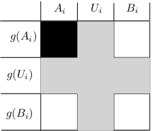
Refer to caption — Figure 1. The sets $A_{i+1}$ , $U_{i+1}$ and $B_{i+1}$ as intersections of the sets $A_{i}$ , $U_{i}$ , $B_{i}$ , $g(A_{i})$ , $g(U_{i})$ , and $g(B_{i})$ . The set $A_{i+1}$ is represented by black, $U_{i+1}$ by grey, and $B_{i+1}$ by white.

$\textrm{(I1)}_{i+1}$ and $\textrm{(I2)}_{i+1}$ are obviously satisfied. The lower bound in $\textrm{(I3)}_{i+1}$ follows from the fact that $g(a)\in A_{i}\cap g(A_{i})$ . The upper bound is then established through the following chain of inequalities:

|A_{i}\cap g(A_{i})|\leqslant|A_{i}|-|A_{i}\cap g(B_{i})|\overset{\mbox{\tiny{\eqref{eq:AigBi}}}}{\leqslant}|A_{i}|-\frac{\alpha n}{2}\;.

This finishes the iterative step.

We now deal with the situation of termination in the step $i_{\mathrm{stop}}<\frac{2}{\alpha}$ . For simplicity, we write $A=A_{i_{\mathrm{stop}}}$ , $B=B_{i_{\mathrm{stop}}}$ , and $U=U_{i_{\mathrm{stop}}}$ . We have

|U|\leqslant 2^{i_{\mathrm{stop}}}\lambda n<2^{2/\alpha}\lambda n\leqslant\frac{1}{4}\mu n\quad\mbox{and similarly}\quad\Delta_{G}(A,B)\leqslant\frac{1}{4}\mu n\;.

(4)

Furthermore, we have

For every

g\in\mathrm{Aut}(G)

, if

g(a^{\prime})\in A

for some

a^{\prime}\in A

, then

g(b^{\prime})\not\in A

for each

b^{\prime}\in B

(5)

We first prove that each vertex $u\in U$ has either almost all its neighbors in $A$ , or in $B$ .

Claim 12.1.

For each $u\in U$ , either $|\mathrm{N}(u)\cap A|\geqslant d-\frac{3}{4}\mu n$ , or $|\mathrm{N}(u)\cap B|\geqslant d-\frac{3}{4}\mu n$ .

Proof of Claim 12.1.

As $d-\frac{3}{4}\mu n>\frac{d}{2}$ , we have that at most one of the assertions of the claim can hold for a given vertex $u\in U$ . Suppose now the statement fails for some $u\in U$ . Then we have

	$\displaystyle\|\mathrm{N}(u)\cap A\|=\|\mathrm{N}(u)\|-\|\mathrm{N}(u)\cap B\|-\|\mathrm{N}(u)\cap U\|$	$\displaystyle>\frac{\mu}{2}n\;,\mbox{and}$		(6)
	$\displaystyle\|\mathrm{N}(u)\cap B\|=\|\mathrm{N}(u)\|-\|\mathrm{N}(u)\cap A\|-\|\mathrm{N}(u)\cap U\|$	$\displaystyle>\frac{\mu}{2}n\;.$		(7)

Let $a\in A$ be arbitrary and take a $g\in\mathrm{Aut}(G)$ such that $g(u)=a$ . We then have $\mathrm{N}(a)=\mathrm{N}(g(u))=g(\mathrm{N}(u))$ , and in particular $g(\mathrm{N}(u)\cap A)\subseteq\mathrm{N}(a)$ .

We claim that there exists an $a^{\prime}\in\mathrm{N}(u)\cap A$ such that $g(a^{\prime})\in A$ . Indeed, if this was not the case, then $g(x)\in B\cup U$ for each $x\in\mathrm{N}(u)\cap A$ . Therefore, we would then have

	$\displaystyle\|\mathrm{N}(a)\cap(B\cup U)\|$	$\displaystyle=\|g(\mathrm{N}(u))\cap(B\cup U)\|\geqslant\|(g(\mathrm{N}(u)\cap A)\cap(B\cup U)\|$
		$\displaystyle=\|g(\mathrm{N}(u)\cap A)\|=\|\mathrm{N}(u)\cap A\|\overset{\mbox{\tiny{\eqref{eq:NuA}}}}{>}\mu n/2\;,$

contradicting (4).

Similarly, using (7) and the fact that $g(\mathrm{N}(u)\cap B)\subseteq g(\mathrm{N}(u))=\mathrm{N}(a)$ , we get that there exists a $b^{\prime}\in\mathrm{N}(u)\cap B$ such that $g(b^{\prime})\in A$ . The properties of $g,a^{\prime}$ and $b^{\prime}$ contradict (5). ∎

By Claim 12.1 we have a partition $U=U_{A}\dot{\cup}U_{B}$ , where $U_{A}=\{u\in U\>:\>\deg(u,A)\geqslant d-\frac{3}{4}\mu n\}$ and $U_{B}=\{u\in U\>:\>\deg(u,B)\geqslant d-\frac{3}{4}\mu n\}$ . Define $V_{1}=A\cup U_{A}$ and $V_{2}=B\cup U_{B}$ . We have $V_{1},V_{2}\neq\emptyset$ . It is straightforward to verify that $\Delta_{G}(V_{1},V_{2})\leqslant\mu n$ . This contradicts the fact that $G$ is $(\mu n)$ -robust. ∎

Observe now that Lemma 12 together with Lemma 11 immediately imply Theorem 8.

We conclude this section with three easy lemmas which are tailored for applications later in the proof of Theorem 25.

Lemma 13.

Suppose that a graph $H$ is $\ell$ -iron. Then the 2-blow-up $2\times H$ is also $\ell$ -iron.²² 2 In fact it is not much more difficult to show that the 2-blow-up is $2\ell$ -iron but $\ell$ -iron connectivity is enough for our purposes and has a clearer proof.

Proof.

Observe first, that the minimum degree of $H$ is at least $2\ell+1$ . Indeed, if there exists a vertex $v$ with $\deg(v)\leqslant 2\ell$ then this vertex can be isolated from the rest of the graph by deletion of at most $\ell$ edges incident with $v$ , and at most $\ell$ vertices in the neighbourhood of $v$ .

Observe that there are two natural vertex disjoint copies of $H$ in $2\times H$ , say $H_{1}$ and $H_{2}$ . Consider any sets $E^{\prime}\subseteq E(2\times H)$ , with $\Delta(E^{\prime})\leqslant\ell$ and $V^{\prime}\subseteq V(2\times H)$ with $|V^{\prime}|\leqslant\ell$ . Since $H$ is $\ell$ -iron, both $H_{1}$ and $H_{2}$ remain connected after the removal of $V^{\prime}$ and $E^{\prime}$ . Since the minimum degree of $H$ is at least $2\ell+1$ , then every vertex of $H_{1}$ has at least $2\ell+1$ neighbours in $H_{2}$ . In particular after the removal of $V^{\prime}$ and $E^{\prime}$ there is still an edge between $H_{1}$ and $H_{2}$ and therefore $(2\times H)\setminus(V^{\prime}\cup E^{\prime})$ is still connected. Therefore $2\times H$ is $\ell$ -iron. ∎

Lemma 14.

Let $R^{\prime}$ be a graph on $k^{\prime}$ vertices. Suppose that there exist sets $L_{1},L_{2}\subseteq V(R^{\prime})$ such that $|L_{1}|\leqslant\sqrt{\varrho}k^{\prime}$ , and $e(L_{2},V(R^{\prime})\setminus(L_{1}\cup L_{2}))\leqslant\varrho k^{\prime 2}$ . If there exists disjoint sets $W_{1},W_{2}\subseteq V(R^{\prime})\setminus(L_{1}\cup L_{2})$ , such that $\mathrm{N}(W_{2})\subseteq L_{1}\cup L_{2}$ , and $\min\{|W_{1}|,|W_{2}|\}>2\sqrt{\varrho}k^{\prime}$ , then $R^{\prime}$ is not $(2\sqrt{\varrho}k^{\prime})$ -iron.

Proof.

Let $L=\{v\in L_{2}\>:\>\deg(v,V(R^{\prime})\setminus(L_{1}\cup L_{2}))\geqslant 2\sqrt{\varrho}k^{\prime}\}$ , and $P=\{v\in V(R^{\prime})\setminus(L_{1}\cup L_{2})\>:\>\deg(v,L_{2})\geqslant 2\sqrt{\varrho}k^{\prime}\}$ . We have $\max\{|L|,|P|\}\leqslant\sqrt{\varrho}k^{\prime}/2$ . In particular,

W_{1}\setminus(L_{1}\cup L\cup P)\neq\emptyset\quad\mbox{and}\quad W_{2}\setminus(L_{1}\cup L\cup P)\neq\emptyset\;.

(8)

Define $E^{\prime}\subseteq E(R^{\prime})$ to be edges running between $L_{2}\setminus L$ and $V(R^{\prime})\setminus(L_{1}\cup L_{2}\cup P)$ . We have $\Delta_{R^{\prime}}(E^{\prime})\leqslant 2\sqrt{\varrho}k^{\prime}$ . By (8), $R^{\prime}$ is not connected after removal of the vertex set $L_{1}\cup L\cup P$ and the edge set $E^{\prime}$ . Indeed, after the removal of $E^{\prime}$ we have that there are no more edges between $W_{2}\setminus(L_{1}\cup L\cup P)$ and $V(R^{\prime})\setminus(W_{2}\cup L_{1}\cup L\cup P)$ . Therefore, $R^{\prime}$ is not $(2\sqrt{\varrho}k^{\prime})$ -iron. ∎

Lemma 15.

Let $H$ be an $n$ -vertex $h$ -strongly connected digraph and let $x,y$ be two distinct vertices of $H$ . Then there exists a (directed) path from $x$ to $y$ of length at most $\frac{n}{h}+1$ .

Proof.

By directed version of Menger’s Theorem (cf. [5, Theorem 7.3.1(b)]), there exist $h$ internally vertex-disjoint directed paths from $x$ to $y$ . Therefore one of these paths must contain at most $\frac{n-2}{h}$ internal vertices and so must have length at most $\frac{n-2}{h}+1\leqslant\frac{n}{h}+1$ . ∎

5. Bipartite case

In this section we give a fine description of dense vertex-transitive graphs which are almost bipartite. Their properties are stated in Lemma 16.

The edit distance $dist(G_{1},G_{2})$ between two $n$ -vertex graph is the number of edges one needs to edit (i.e. to either remove or add) to get $G_{2}$ from $G_{1}$ , minimized over all identification of $V(G_{1})$ with $V(G_{2})$ . Given an $n$ -vertex graph $G$ , we say that it is $\varepsilon$ -close to a graph property $\mathcal{P}$ if there exists an $n$ -vertex graph $H\in\mathcal{P}$ such that $dist(G,H)<\varepsilon n^{2}$ . Otherwise we say that it is $\varepsilon$ -far from $\mathcal{P}$ .

Lemma 16.

Let $c\in(0,\frac{1}{17})$ be arbitrary. Suppose that $G$ is a $cn$ -iron vertex-transitive graph $G$ on $n$ vertices which is $c^{4}$ -close to bipartiteness. Then there exist a bipartition $V(G)=A\dot{\cup}B$ such that $|A|=|B|$ , for each $u\in A$ and each $v\in B$ we have $\deg(u,A)\leqslant 6c^{2}n$ , and $\deg(v,B)\leqslant 6c^{2}n$ . Furthermore, we have $g(A)=A$ or $g(A)=B$ for each $g\in\mathrm{Aut}(G)$ .

Proof.

We write $\Delta$ for the valency of $G$ . Observe that since $G$ is $cn$ -robust, then $\Delta\geqslant cn$ . Let $A\dot{\cup}B=V(G)$ be the bipartition which maximizes $e(A,B)$ . We have

e(A)+e(B)<c^{4}n^{2}\;.

(9)

We claim that

\min\{|A|,|B|\}\geqslant\frac{n}{3}\;.

(10)

Indeed, suppose for contradiction that, for example, $|A|>\frac{2n}{3}$ and $|B|<\frac{n}{3}$ . Counting $e(A,B)$ in two ways we arrive to $\sum_{v\in A}\deg(v)-2e(A)=\sum_{v\in B}\deg(v)-2e(B)$ , and therefore

\frac{2\Delta n}{3}<\Delta|A|\leqslant\Delta|B|+2c^{4}n^{2}<\frac{\Delta n}{3}+2c^{4}n^{2},

a contradiction as $\Delta\geqslant cn$ and $c$ is sufficiently small. This proves (10).

Define $A^{\prime}=\{v\in A\>:\>\deg(v,A)\geqslant c^{2}n\}$ , and $B^{\prime}=\{v\in B\>:\>\deg(v,B)\geqslant c^{2}n\}$ . By (9) we have $|A^{\prime}|+|B^{\prime}|<2c^{2}n$ . Together with (10) this gives that

A\setminus A^{\prime}\neq\emptyset\quad\mbox{and}\quad B\setminus B^{\prime}\neq\emptyset\;.

(11)

Claim 16.1.

For each $g\in\mathrm{Aut}(G)$ we either have $|A\cap g(A)|\geqslant|A|-5c^{2}n$ or $|A\cap g(B)|\geqslant|A|-5c^{2}n$ . Also, for each $g\in\mathrm{Aut}(G)$ we either have $|B\cap g(A)|\geqslant|B|-5c^{2}n$ or $|B\cap g(B)|\geqslant|B|-5c^{2}n$ .

Proof of Claim 16.1.

It is enough to prove the first statement.

We start with some general calculations. We shall later use them to show that if $g\in\mathrm{Aut}(G)$ failed to fulfil the assertions we would get a contradiction to $cn$ -iron connectivity.

Let $\tilde{A}=A\setminus A^{\prime}$ and $\tilde{B}=B\setminus B^{\prime}$ . Consider the partition $V(G)=X\dot{\cup}Y\dot{\cup}U$ , where $X=(\tilde{A}\cap g(\tilde{A}))\cup(\tilde{B}\cap g(\tilde{B}))$ , $Y=(\tilde{A}\cap g(\tilde{B}))\cup(\tilde{B}\cap g(\tilde{A}))$ , and $U=V(G)\setminus(X\cup Y)$ . We have

|U|\leqslant|A^{\prime}|+|B^{\prime}|+|g(A^{\prime})|+|g(B^{\prime})|\leqslant 4c^{2}n\leqslant cn\;.

(12)

We claim that

\Delta_{G}(X,Y)\leqslant cn\;.

(13)

To prove this it suffices to prove that

\max\left\{\Delta_{\tilde{A}\tilde{A},\tilde{A}\tilde{B}},\Delta_{\tilde{A}\tilde{A},\tilde{B}\tilde{A}},\Delta_{\tilde{B}\tilde{B},\tilde{A}\tilde{B}},\Delta_{\tilde{B}\tilde{B},\tilde{B}\tilde{A}},\Delta_{\tilde{A}\tilde{B},\tilde{A}\tilde{A}},\Delta_{\tilde{B}\tilde{A},\tilde{A}\tilde{A}},\Delta_{\tilde{A}\tilde{B},\tilde{B}\tilde{B}},\Delta_{\tilde{B}\tilde{A},\tilde{B}\tilde{B}}\right\}\leqslant\frac{cn}{2}\;,

(14)

where $\Delta_{CD,EF}=\max\{\deg(v,E\cap g(F)):v\in C\cap g(D)\}$ defines the eight new symbols above. Here we only bound the first two terms; the methods to this end apply to the remaining six as well. To prove that $\Delta_{\tilde{A}\tilde{A},\tilde{A}\tilde{B}}\leqslant\frac{cn}{2}$ , consider an arbitrary $v\in\tilde{A}\cap g(\tilde{A})$ . We have $v\not\in A^{\prime}$ . We then have $\deg(v,\tilde{A}\cap g(\tilde{B}))\leqslant\deg(v,\tilde{A})\leqslant\deg(v,A)<c^{2}n$ , where the last inequality follows from the definition of the set $A^{\prime}$ . To bound $\Delta_{\tilde{A}\tilde{A},\tilde{B}\tilde{A}}$ we again consider an arbitrary $v\in\tilde{A}\cap g(\tilde{A})$ . We have

\deg(v,\tilde{B}\cap g(\tilde{A}))=\deg(g^{-1}(v),g^{-1}(\tilde{B})\cap g^{-1}(g(\tilde{A})))=\deg(g^{-1}(v),g^{-1}(\tilde{B})\cap\tilde{A})\leqslant\deg(g^{-1}(v),\tilde{A})\;.

We observe that $g^{-1}(v)\in g^{-1}(\tilde{A})\cap g^{-1}(g(\tilde{A}))\subseteq\tilde{A}$ , and the bound follows by the definition of the set $A^{\prime}$ .

Suppose now that the statement of the Claim fails for $g\in\mathrm{Aut}(G)$ . We then have $X\neq\emptyset$ and $Y\neq\emptyset$ . Indeed, to show for example that $X\neq\emptyset$ , we note that

|X|\geqslant|A\cap g(A)|-|A^{\prime}|-|g(A^{\prime})|>5c^{2}n-2c^{2}n-2c^{2}n>0\;.

Let $E^{\prime}$ be the edges of $G$ running between $X$ and $Y$ . Now if we remove $U$ and $E^{\prime}$ from $G$ we get a disconnected graph. Together with the bounds (12) and (13) this proves that $G$ is not $cn$ -iron, a contradiction. ∎

Claim 16.2.

For every $v\in A$ we have $\deg(v,A)\leqslant 6c^{2}n$ . Also, for every $v\in B$ we have $\deg(v,B)\leqslant 6c^{2}n$ .

Proof of Claim 16.2.

By symmetry, it suffices to prove the first part of the statement. Let $w\in B\setminus B^{\prime}$ be arbitrary; such a choice is possible by (11). Let $v\in A$ and take $g\in\mathrm{Aut}(G)$ be such that $g(v)=w$ . Let $P=\mathrm{N}(v)\cap A$ , and $Q=\mathrm{N}(v)\cap B$ . Suppose for contradiction that $|P|>6c^{2}n$ . Since the bipartition $A\dot{\cup}B$ was chosen to maximize $e(A,B)$ , we must have $|Q|\geqslant\frac{cn}{2}$ . Since $\mathrm{N}(w)=g(P)\cup g(Q)$ and since also $w\not\in B^{\prime}$ we have that $|g(A)\cap A|\geqslant|g(P)\cap A|>5c^{2}n$ and so $|g(A)\cap B|<|B|-5c^{2}n$ . Similarly, we also have $|g(B)\cap A|\geqslant|g(Q)\cap A|>5c^{2}n$ and so $|g(B)\cap B|<|B|-5c^{2}n$ . But these contradict Claim 16.1. ∎

Claim 16.3.

For every $g\in\mathrm{Aut}(G)$ we either have $A\cap g(A)=\emptyset$ , or $A\cap g(B)=\emptyset$ . Likewise, we have $B\cap g(A)=\emptyset$ , or $B\cap g(B)=\emptyset$ .

Proof of Claim 16.3.

Let $C,D\in\{A,B\}$ . Let $C^{\prime}=V(G)\setminus C$ , and $D^{\prime}=V(G)\setminus D$ . (Thus $C^{\prime},D^{\prime}\in\{A,B\}$ .)

Suppose that $C\cap g(D)\neq\emptyset$ . We can take a $v\in C$ with $g^{-1}(v)\in D$ . Using Claim 16.2 for $g^{-1}(v)$ , and then for $v$ we get.

	$\displaystyle 6c^{2}n\geqslant$	$\displaystyle\deg(g^{-1}(v),D)=\|\mathrm{N}(g^{-1}(v))\cap D\|=\|\mathrm{N}(v)\cap g(D)\|\geqslant\|\mathrm{N}(v)\cap C^{\prime}\cap g(D)\|$
		$\displaystyle=\|\mathrm{N}(v)\cap C^{\prime}\|-\|\mathrm{N}(v)\cap C^{\prime}\cap g(D^{\prime})\|\geqslant\|\mathrm{N}(v)\|-\|\mathrm{N}(v)\cap C\|-\|C^{\prime}\cap g(D^{\prime})\|$
		$\displaystyle\geqslant\Delta-6c^{2}n-\|C^{\prime}\cap g(D^{\prime})\|\geqslant cn-6c^{2}n-\|C^{\prime}\cap g(D^{\prime})\|.$

Thus $|C^{\prime}\cap g(D^{\prime})|\geqslant cn-12c^{2}n>5c^{2}n$ . Hence $C^{\prime}\cap g(D^{\prime})\neq\emptyset$ . Repeating the previous argument for $C^{\prime}$ and $D^{\prime}$ yields $|C\cap g(D)|>5c^{2}n$ .

Therefore for every $C,D\in\{A,B\}$ we have

|C\cap g(D)|=0\text{ or }|C\cap g(D)|>5c^{2}n\;.

(15)

We use this for $C=A$ and $D=B$ . We get that $|A\cap g(B)|=0$ , or $|A\cap g(B)|>5c^{2}n$ . We are done in the former case. In the latter case, we have $|A\cap g(A)|<|A|-5c^{2}n$ . Claim 16.1 then gives that $|A\cap g(B)|>|A|-5c^{2}n$ . Using again (15), this time with $C=A$ , $D=A$ , we get that $|A\cap g(A)|=0$ . ∎

Claims 16.2 and 16.3 show that the bipartition $A\dot{\cup}B$ satisfies the conclusion of Lemma 16. ∎

Remark 17.

In the above proof we showed that the partition maximizing $e(A,B)$ satisfies the conclusion of Lemma 16. In fact we only used the following two properties of the partition:

(1)

The partition satisfies (9).
(2)

For every $v\in A$ we have $\deg(v,A)\leqslant\deg(v,B)$ and for every $v\in B$ we have that $\deg(v,B)\leqslant\deg(v,A)$ .

In particular any partition satisfying the above two properties also satisfies the conclusion of Lemma 16. This fact will be important in the proof of Theorem 27 which provides an algorithmic version of Theorem 2.

Remark 18.

Note that the bipartite subgraph $G[A,B]$ obtained from the partition $A\dot{\cup}B$ given by Lemma 16 by removing all edges within the parts $A$ and $B$ is itself vertex-transitive. Indeed observe that for any automorphism $g\in\mathrm{Aut}(G)$ and any edge $e$ between the parts $A$ and $B$ we have that $g(e)$ also lies between these parts. Therefore every automorphism of $G$ restricted to $G[A,B]$ is also an automorphism and so $G[A,B]$ is vertex-transitive.

6. Szemerédi’s Regularity Lemma

Szemerédi’s Regularity Lemma is one of the main tools in our proof of Theorem 2. In this section we collect all the tools related to the Regularity Lemma that we will need. For surveys on the Regularity Lemma and its applications we refer the reader to [18, 15, 17, 21].

Before stating the lemma, we need to introduce some more notation. The density of a bipartite graph $G$ with vertex classes $A$ and $B$ is defined to be $d_{G}(A,B)=\frac{e(A,B)}{|A||B|}$ . We sometimes write $d(A,B)$ for $d_{G}(A,B)$ if this is unambiguous. Given $\varepsilon>0$ , we say that $G$ is $\varepsilon$ -regular if for all subsets $X\subseteq A$ and $Y\subseteq B$ with $|X|\geqslant\varepsilon|A|$ and $|Y|\geqslant\varepsilon|B|$ we have that $|d(X,Y)-d(A,B)|<\varepsilon$ . Given $d\in[0,1]$ , we say that $G$ is $(\varepsilon,d)$ -regular if it is $\varepsilon$ -regular of density at least $d$ . We also say that $G$ is $(\varepsilon,d)$ -super-regular if it is $\varepsilon$ -regular and furthermore $d_{G}(a)\geqslant d|B|$ for all $a\in A$ and $d_{G}(b)\geqslant d|A|$ for all $b\in B$ . Given partitions $V_{0}\dot{\cup}V_{1}\dot{\cup}\ldots\dot{\cup}V_{k}$ and $U_{1}\dot{\cup}\ldots\dot{\cup}U_{\ell}$ of the vertex set of some graph, we say that $V_{0}\dot{\cup}V_{1}\dot{\cup}\ldots\dot{\cup}V_{k}$ refines $U_{1}\dot{\cup}\ldots\dot{\cup}U_{\ell}$ if for all $i$ with $1\leqslant i\leqslant k$ , there is some $1\leqslant j\leqslant\ell$ with $V_{i}\subseteq U_{j}$ . Note that this is weaker than the usual notion of refinement as we do not require $V_{0}$ to be contained in any $U_{j}$ . We will use the following degree form of Szemerédi’s Regularity Lemma [28]:

Lemma 19 (Regularity Lemma; Degree form).

Given $\varepsilon\in(0,1)$ and integers $N^{\prime},\ell$ , there are integers $N=N(\varepsilon,N^{\prime},\ell)$ and $n_{0}=n_{0}(\varepsilon,N^{\prime},\ell)$ such that if $G$ is any graph on $n\geqslant n_{0}$ vertices, $d\in[0,1]$ is any real number, and $U_{1},\ldots,U_{\ell}$ is any partition of the vertex set of $G$ , then there is a partition of the vertex set of $G$ into $k+1$ classes $V_{0}\dot{\cup}V_{1}\dot{\cup}\ldots\dot{\cup}V_{k}$ , and a spanning subgraph $G^{\prime}$ of $G$ with the following properties:

(i)

$N^{\prime}\leqslant k\leqslant N$ ;
(ii)

$V_{0}\dot{\cup}V_{1}\dot{\cup}\ldots\dot{\cup}V_{k}$ refines $U_{1}\dot{\cup}\ldots\dot{\cup}U_{\ell}$ ;
(iii)

$|V_{0}|\leqslant\varepsilon n,|V_{1}|=\cdots=|V_{k}|=m$ ;
(iv)

$\deg_{G^{\prime}}(v)\geqslant\deg_{G}(v)-(d+\varepsilon)n$ for every $v\in V(G)\setminus V_{0}$ ;
(v)

$G^{\prime}[V_{i}]$ is empty for every $0\leqslant i\leqslant k$ , and no edges of $G^{\prime}$ are incident with $V_{0}$ ;
(vi)

all pairs $(V_{i},V_{j})$ with $1\leqslant i<j\leqslant k$ are $\varepsilon$ -regular with density either 0 or at least $d$ .

We call $V_{1},\ldots,V_{k}$ the clusters of the partition, $V_{0}$ the exceptional set and the vertices of $G$ in $V_{0}$ the exceptional vertices. The reduced graph $R=R_{G^{\prime}}$ of $G$ with respect to the above partition and the parameters $\varepsilon$ and $d$ is the graph whose vertices are the clusters $V_{1}\ldots,V_{k}$ in which $V_{i}V_{j}$ is an edge precisely when the pair $(V_{i},V_{j})$ has density at least $d$ in $G^{\prime}$ .

Remark 20.

It turns out that for the proofs of Theorems 25 and 26 (see below) we need to work with two threshold densities $d_{1}<d_{2}$ of the reduced graph. The degree form of the Regularity Lemma can be adapted in order to accommodate this need. In particular we can get a partition $V_{0}\dot{\cup}V_{1}\dot{\cup}\ldots\dot{\cup}V_{k}$ of the vertex set of $G$ and spanning subgraphs $G_{1},G_{2}$ of $G$ such that properties (i)–(vi) of the Regularity Lemma hold for both $G_{1}$ and $G_{2}$ with the corresponding densities $d_{1}$ and $d_{2}$ . (This can be deduced in the same way as the degree form of the Regularity Lemma is deduced from the standard form.)

For further use, we also recall the following well-known facts. The next lemma says that large sub-pairs of regular pairs are regular.

Lemma 21.

Let $(A,B)$ be an $(\varepsilon,d)$ -regular pair with $\varepsilon\leqslant d/2$ and let $A^{\prime}$ and $B^{\prime}$ be subsets of $A$ and $B$ of sizes $|A^{\prime}|\geqslant|A|/3$ and $|B^{\prime}|\geqslant|B|/3$ . Then $(A^{\prime},B^{\prime})$ is $(3\varepsilon,d/2)$ -regular.

Given any bounded degree subgraph $H$ of the reduced graph $R$ we can make the pairs corresponding to its edges super-regular by removing a small fraction of the vertices of each cluster to the exceptional set. We will only need this fact in the case that $H$ is a matching.

Lemma 22.

Suppose $0<4\varepsilon<d\leqslant 1$ and let $V_{0}\dot{\cup}V_{1}\dot{\cup}\ldots\dot{\cup}V_{k}$ be a partition of a graph $G$ as given by the Regularity Lemma. Let $R$ be the reduced graph with respect to this partition and the parameters $\varepsilon$ and $d$ . Let $M$ be a matching in $R$ . Then we can move exactly $\varepsilon m$ vertices from each cluster $V_{i}$ into $V_{0}$ such that each pair of clusters corresponding to an edge of $M$ is $(2\varepsilon,d/2)$ -super-regular while each pair of clusters corresponding to an edge of $R$ is $(2\varepsilon,d/2)$ -regular.

Given an $(\varepsilon,d)$ -super-regular pair $(A,B)$ , we will often need to isolate a small sub-pair that maintains super-regularity in any sub-pair that contains it. For $A^{*}\subseteq A$ and $B^{*}\subseteq B$ we say that $(A^{*},B^{*})$ is an $(\varepsilon^{*},d^{*})$ -ideal for $(A,B)$ if for any $A^{*}\subseteq A^{\prime}\subseteq A$ and $B^{*}\subseteq B^{\prime}\subseteq B$ the pair $(A^{\prime},B^{\prime})$ is $(\varepsilon^{*},d^{*})$ -super-regular. The following lemma shows that ideals exist.

Lemma 23 ([8, Lemma 15]).

Suppose $0<\varepsilon\ll\theta,d<1/2$ , and let $(A,B)$ be an $(\varepsilon,d)$ -super-regular pair with $|A|=|B|=m$ , where $m$ is sufficiently large. Then there exists subsets $A^{*}\subseteq A$ and $B^{*}\subseteq B$ of sizes $\theta m$ such that $(A^{*},B^{*})$ is an $(\varepsilon/\theta,\theta d/4)$ -ideal for $(A,B)$ .

The proof of the above lemma given in [8] is probabilistic. (It proves that random subsets of sizes $\theta m$ have the required property with high probability.) For finding the Hamilton cycle efficiently in Theorem 27 below we will also need a ‘constructive’ proof of this lemma. We proceed to give such a proof.

Proof of Lemma 23.

By using a more general version of the Lemma 21, it is enough to construct subsets $A^{*}\subseteq A$ and $B^{*}\subseteq B$ of sizes $\theta m$ such that every vertex $a\in A$ has $\deg(a,B^{*})\geqslant\theta dm/4$ and every vertex $b\in B$ has $\deg(b,A^{*})\geqslant\theta dm/4$ . By symmetry, it is enough to show how to construct a subset $A^{*}\subseteq A$ of size $\theta m$ such that very vertex $b\in B$ has $\deg(b,A^{*})\geqslant\theta dm/4$ . We will construct this set $A^{*}$ by adding to it one vertex at every step. At each step we will say that a vertex $b$ of $B$ is unhappy if it has $k<\theta dm/4$ neighbours in $A^{*}$ . If a vertex $b$ is unhappy we will define its unhappiness $u(b)$ to be $u(b)=\sum_{r=k+1}^{\theta dm/4}2^{-r}$ . Otherwise we define its unhappiness $u(b)$ to be equal to 0. We also denote by $U$ the total unhappiness $U=\sum_{b\in B}u(b)$ of vertices of $B$ . Observe that if in the next step we add to $A^{*}$ a neighbour of $b$ then the unhappiness of $b$ is reduced by at least $u(b)/2$ . Note also that if a vertex $b$ is unhappy, then it has at least $dm-\theta dm/4\geqslant dm/2$ neighbours outside of $A^{*}$ . We now give to every edge joining $b$ to a vertex of $A\setminus A^{*}$ a weight equal to $u(b)/2$ . Then the total weight on these edges is at least $\sum_{b\in B}u(b)dm/4=Udm/4$ . In particular there is a vertex $a\in A\setminus A^{*}$ where the total weight on its incident edges is at least $Ud/4$ . Adding this vertex to $A^{*}$ we get that the new total unhappiness is at most $(1-d/4)U$ . Initially the total unhappiness was at most $m$ . So after $\theta m$ steps the total unhappiness is at most $(1-d/4)^{\theta m}m\leqslant me^{-\theta md/4}<2^{-\theta dm/4}$ , when $m$ is sufficiently large. But no unhappy vertex can have unhappiness less than $2^{-\theta dm/4}$ . It follows that after $\theta m$ steps there is no unhappy vertex in $B$ , as required. ∎

We will also need the following ‘blow-up’-type statement.

Lemma 24.

Suppose $0<\varepsilon\ll d$ and let $(A,B)$ be an $(\varepsilon,d)$ -super-regular pair with $|A|=|B|$ . Let $a\in A$ and $b\in B$ . Then $A\cup B$ contains a Hamilton path with endvertices $a$ and $b$ .

Proof.

The lemma follows from the Blow-up Lemma of Komlós, Sárközy and Szemerédi [15]. We need to deal with one minor difficulty which does not allow a direct application of the Blow-up Lemma, namely that we are prescribing exactly the images $a$ and $b$ of the endvertices of the Hamilton path.

Recall that by [15, Remark 13] we can impose additional restriction on a small number of target sets of vertices of the graph we are trying to embed in the super-regular pair. We thus proceed as follows.

We can assume that $|A|$ is sufficiently large. Otherwise, setting $\varepsilon$ small, we can force $(A,B)$ to form a complete bipartite graph, and then the statement is trivial.

Let $A^{\prime}\subseteq A$ and $B^{\prime}\subseteq B$ be the neighbourhood of $b$ and $a$ , respectively. We have $|A^{\prime}\setminus\{a\}|\geqslant\frac{d|A|}{2}$ , and $|B^{\prime}\setminus\{b\}|\geqslant\frac{d|B|}{2}$ . Observe also, that the pair $(A\setminus\{a\},B\setminus\{b\})$ is $(2\varepsilon,\frac{d}{2})$ -super-regular. By the Blow-up Lemma we can find a Hamilton path $P$ in the pair $(A\setminus\{a\},B\setminus\{b\})$ . Furthermore, by [15, Remark 13] we can require the endvertices of the path to lie in the sets $A^{\prime}$ and $B^{\prime}$ . The path $aPb$ is a Hamilton path in $(A,B)$ satisfying the assertions of the lemma. ∎

7. Hamilton cycles in iron connected vertex-transitive graphs

In this section, we prove a stronger version of Theorem 2 under the additional assumption of high iron connectivity of the host graph. This is stated in Theorem 25 in the non-bipartite setting, and in Theorem 26 in the bipartite setting.

The basic idea is to follow Łuczak’s ‘connected matching argument’ [24]. The novel ingredient in our work is an innocent looking modification of this technique: we observe that we can extend the argument to work with fractional matchings as well. This allows one to use the LP-duality. We believe that this observation will find further important applications in the future. (After the first version of this manuscript was posted on the arXiv, we learned that Rödl and Ruciński announced a solution of a certain Dirac-type problem for hypergraphs using Farkas’ Lemma, an approach similar to our linear programming approach. The corresponding paper was posted later in the arXiv [2].) The use of the LP-duality in conjunction with the Regularity Lemma originated in discussion of Jan Hladký with Dan Král’ and Diana Piguet. (As it was pointed to us by Deryk Osthus, the full strength of the LP-duality machinery is not needed. In [20] it is shown that every dense almost regular graph has a reduced graph with an almost perfect matching and this suffices in our setting.)

Theorem 25.

For every $\beta,\gamma>0$ and every $C\in\mathbb{N}$ , there exists an $N_{1}$ such that every $\beta n$ -iron vertex-transitive graph of order $n\geqslant N_{1}$ which is $\beta$ -far from bipartiteness is $C$ -pathitionable with an exceptional set $U\subseteq V(G)$ with $|U|<\gamma n$ .

Theorem 26.

For every $c\in(0,\frac{1}{17})$ , $\gamma>0$ and $C\in\mathbb{N}$ there an exists $N_{2}$ such that for every vertex-transitive graph $G$ of order $n\geqslant N_{2}$ the following holds. Suppose $G$ is $cn$ -iron and $c^{4}$ -close to bipartiteness. Let $A\dot{\cup}B$ be the bipartition of $G$ given by Lemma 16. Then there exists a set $U\subseteq V(G)$ with $|U|<\gamma n$ such that $G$ is $C$ -bipathitionable with exceptional set $U$ with respect to the partition $A\dot{\cup}B$ .

After proving Theorem 25 in detail below, we indicate necessary changes to make an analogous proof of Theorem 26 work as well.

Proof of Theorem 25.

We begin by fixing additional constants $\varepsilon,d_{1},d_{2},\gamma_{1},\gamma_{2}$ satisfying

0<\varepsilon\ll d_{1}\ll\gamma_{1}\ll\gamma_{2}\ll d_{2}\ll\gamma,\beta.

Let $N^{\prime}=1/\varepsilon$ . Let $N(\varepsilon,N^{\prime},1)$ and $n_{0}(\varepsilon,N^{\prime},1)$ be the numbers given by the Regularity Lemma. Set

n_{0}=\max\left\{\frac{N(\varepsilon,N^{\prime},1)}{\gamma_{1}},n_{0}(\varepsilon,N^{\prime},1)\right\}\;.

(16)

Let $G$ be any $\beta n$ -iron connected vertex-transitive graph on $n\geqslant n_{0}$ vertices of valency $\Delta$ . Apply the Regularity Lemma (see also Remark 20) with parameters $\varepsilon,N^{\prime},\ell=1$ and $d_{1},d_{2}$ to $G$ to obtain a partition $V_{0}\dot{\cup}V_{1}\dot{\cup}\ldots\dot{\cup}V_{k}$ of $V(G)$ . Let $G_{1},G_{2}\subseteq G$ be the spanning subgraphs of $G$ given by the Regularity Lemma corresponding to the densities $d_{1}$ and $d_{2}$ respectively. Let also $R_{1}$ and $R_{2}$ be the reduced graphs of $G$ with respect to the above partition, the parameters $\varepsilon$ and $d_{1},d_{2}$ and the subgraphs $G_{1}$ and $G_{2}$ respectively. We write $m=|V_{1}|$ .

We first claim that $R_{1}$ has a large fractional matching.

Claim 25.1.

$\nu^{*}(R_{1})\geqslant(1-\frac{\gamma_{1}}{2})\frac{k}{2}$ .

Proof of Claim 25.1.

Observe that by Lemma 5 we have that $\tau^{*}(G)=n/2$ . We also have that

e(G_{1})\geqslant e(G)-(d_{1}+\varepsilon)n^{2}\geqslant\left(1-\frac{\gamma_{1}}{2}\right)e(G)\;,

where in the first inequality we used properties (iii)–(v) of the Regularity Lemma and in the second one we used the fact that $e(G)\geqslant\beta n^{2}/2$ . By Lemma 4 we obtain that $\tau^{*}(G_{1})\geqslant(1-\frac{\gamma_{1}}{2})\frac{n}{2}$ . Observe that $\nu^{*}(G_{1})=\nu^{*}(G_{1}-V_{0})$ by property (v) of the Regularity Lemma. Therefore, combining Lemma 7 with Theorem 3 (a) we have

\nu^{*}(R_{1})\geqslant\frac{\nu^{*}(G_{1})}{m}=\frac{\tau^{*}(G_{1})}{m}\geqslant\left(1-\frac{\gamma_{1}}{2}\right)\frac{n}{2m}\geqslant\left(1-\frac{\gamma_{1}}{2}\right)\frac{k}{2}\;.\qed

The density $d_{1}$ was used to find a large matching in $R_{1}$ (cf. Claim 25.1). On the other hand, it is more convenient to work with the higher threshold density $d_{2}$ to infer some connectivity properties of certain graphs that will be derived from $R_{2}$ (most importantly, to deduce Claim 25.5).

Since $G$ is $\beta n$ -iron and $\varepsilon,d_{2}\ll\beta$ , properties (iii) and (iv) of the Regularity Lemma (for the density $d_{2}$ ) imply that $G_{2}[V\setminus V_{0}]$ is $(\beta n/2)$ -iron. We claim that the iron connectivity is inherited by the reduced graph $R_{2}$ as well.

Claim 25.2.

$R_{2}$ is $(\beta k/2)$ -iron.

Proof of Claim 25.2.

Indeed, suppose we could disconnect $R_{2}$ by removing a set of clusters $S$ of size at most $\beta k/2$ together with an edge set $F\subseteq E(R_{2})$ with $\Delta(F)\leqslant\beta k/2$ . Let $E^{\prime}\subseteq E(G_{2}[V\setminus V_{0}])$ be the set of edges contained in the regular pairs corresponding to $F$ . Then we could also disconnect $G_{2}[V\setminus V_{0}]$ by removing all vertices belonging to the clusters of $S$ together with the edge set $E^{\prime}$ . However, the clusters of $S$ contain at most $\beta km/2\leqslant\beta n/2$ vertices and also $\Delta(E^{\prime})\leqslant\beta km/2\leqslant\beta n/2$ . This would contradict the $(\beta n/2)$ -iron connectivity of $G_{2}[V\setminus V_{0}]$ . ∎

For each $1\leqslant i\leqslant k$ , we arbitrarily partition $V_{i}$ into two parts $V_{i}^{1}$ and $V_{i}^{2}$ of equal sizes. In the case that the $V_{i}$ ’s have odd sizes, then before the partitioning we move an arbitrary vertex from each cluster into $V_{0}$ . We denote the new exceptional set obtained by $V_{0}^{\prime}$ . We also define a new graph $R^{\prime}_{1}$ on vertex set $\{V_{1}^{1},V_{1}^{2},\ldots,V_{k}^{1},V_{k}^{2}\}$ where $V_{i}^{s}$ is adjacent to $V_{j}^{t}$ if and only if $V_{i}$ was adjacent to $V_{j}$ in $R_{1}$ . Similarly, we define a graph $R^{\prime}_{2}$ on the same vertex set as $R^{\prime}_{1}$ to be the 2-blow-up of $R_{2}$ . By Lemma 21 every edge of $R^{\prime}_{1}$ corresponds to a $(3\varepsilon,d_{1}/2)$ -regular pair, and every edge of $R^{\prime}_{2}$ corresponds to a $(3\varepsilon,d_{2}/2)$ -regular pair. We have $R_{1}^{\prime}=2\times R_{1}$ , $R_{2}^{\prime}=2\times R_{2}$ , and $R^{\prime}_{2}\subseteq R^{\prime}_{1}$ . Consider a matching $M$ in $R^{\prime}_{1}$ of weight at least $(1-\frac{\gamma_{1}}{2})k$ . Such a matching exists by Claim 25.1 and by Lemma 6.

Observe that $R^{\prime}_{1}$ is itself a reduced graph of the partition $V_{0}^{\prime}\dot{\cup}V_{1}^{1}\dot{\cup}V_{1}^{2}\dot{\cup}\ldots\dot{\cup}V_{k}^{1}\dot{\cup}V_{k}^{2}$ with respect to the parameters $3\varepsilon$ and $d_{1}/2$ and some subgraph $G_{1}^{\prime}$ of $G$ . In particular, we can apply Lemma 22 to $R_{1}^{\prime}$ and the matching $M$ to remove exactly $3\varepsilon m$ vertices from each cluster of $R_{1}^{\prime}$ so that every pair of clusters corresponding to an edge of $M$ is $(6\varepsilon,d_{1}/4)$ -super-regular while every pair of clusters corresponding to an edge of $R_{1}^{\prime}$ is $(6\varepsilon,d_{1}/4)$ -regular. It also follows that every pair of these modified clusters corresponding to an edge of $R^{\prime}_{2}$ is $(6\varepsilon,d_{2}/4)$ -regular.

We now move all clusters of $R^{\prime}_{1}$ which are not incident to the matching $M$ into the exceptional set. This modification is also performed in the graph $R^{\prime}_{2}$ . Let ${k^{\prime}}$ be the number of clusters of this modified graph $R^{\prime}_{1}$ , and ${m^{\prime}}$ be the size of each of its clusters, which are denoted by $V^{\prime}_{1},\ldots,V^{\prime}_{k^{\prime}}$ (and we write $V^{\prime}_{0}$ for the exceptional set).

The modified graph $R^{\prime}_{2}$ is obtained from $2\times R_{2}$ by removing a small number of vertices. From Claim 25.2 and Lemma 13 we get that $2\times R_{2}$ is $(\beta k/2)$ -iron. Therefore

R^{\prime}_{2}

(\frac{\beta{k^{\prime}}}{5})

-iron.

(17)

From now on, all references to $R_{1}^{\prime},R_{2}^{\prime}$ and the matching $M$ will be to these modified versions.

By the above, there is a partition of the vertices of $G$ into ${k^{\prime}}+1$ classes $V^{\prime}_{0}\dot{\cup}V^{\prime}_{1}\dot{\cup}\ldots\dot{\cup}V^{\prime}_{k^{\prime}}$ , and a spanning subgraph $G^{\prime}$ of $G$ with the following properties:

(a)

$1/\varepsilon\leqslant{k^{\prime}}\leqslant 2N(\varepsilon,N^{\prime},1)\leqslant 2\gamma_{1}n$ (using the bound (16)).
(b)

$|V^{\prime}_{0}|\leqslant 2\gamma_{1}n,|V^{\prime}_{1}|=\cdots=|V^{\prime}_{k^{\prime}}|={m^{\prime}}$ .
(c)

$\deg_{G^{\prime}}(v)\geqslant\deg_{G}(v)-3\gamma_{1}n$ for every $v\in V(G)\setminus V^{\prime}_{0}$ .
(d)

$G^{\prime}[V^{\prime}_{i}]$ is empty for every $0\leqslant i\leqslant{k^{\prime}}$ .
(e)

All pairs $(V^{\prime}_{i},V^{\prime}_{j})$ with $1\leqslant i<j\leqslant{k^{\prime}}$ are $6\varepsilon$ -regular with density either 0 or at least $d_{1}/4$ .
(f)

There is a $\beta k^{\prime}/5$ -iron graph $R^{\prime}_{2}$ on vertex set $V^{\prime}_{1},\ldots,V^{\prime}_{k^{\prime}}$ such that every edge of $R^{\prime}_{2}$ corresponds to a $(6\varepsilon,d_{2}/4)$ -regular pair in $G$ .
(g)

There is a perfect matching $M$ on the complete graph formed by the clusters $V^{\prime}_{1},\ldots,V^{\prime}_{k^{\prime}}$ . Further, every edge of $M$ corresponds to a $(6\varepsilon,d_{1}/4)$ -super-regular pair in $G$ .

If $XY\in M$ , then we call $Y$ the partner of $X$ . Let us denote the edges of $M$ by $A_{i}B_{i}$ for $1\leqslant i\leqslant{k^{\prime}}/2$ . Using Lemma 23 with $\theta=d_{1}^{2}$ for each $1\leqslant i\leqslant{k^{\prime}}/2$ , we find $A_{i}^{*}$ and $B_{i}^{*}$ with $|A_{i}^{*}|=|B_{i}^{*}|=d_{1}^{2}{m^{\prime}}$ , such that $(A_{i}^{*},B_{i}^{*})$ is an $(6\varepsilon/d_{1}^{2},d_{1}^{3}/16)$ -ideal for $(A_{i},B_{i})$ .

We now define the exceptional set $U$ in the statement of the theorem as follows:

U=V^{\prime}_{0}\cup\bigcup_{i=1}^{{k^{\prime}}/2}(A_{i}^{*}\cup B_{i}^{*}).

Observe that

|U|\leqslant 2\gamma_{1}n+d_{1}^{2}n\leqslant 3\gamma_{1}n<\gamma n.

Suppose now that we are in the setting of the theorem, that is, we are given distinct vertices $x_{1},y_{1},\ldots,x_{\ell},y_{\ell}\in V(G)\setminus U$ (where $1\leqslant\ell\leqslant C$ ), and our task is to find a system $\mathcal{S}$ of $\ell$ vertex-disjoint of paths that partition $V(G)$ . Furthermore it is required that $x_{j}$ and $y_{j}$ are the endvertices of the $j$ -th path.

Our first aim is to find a system $\mathcal{S}^{\prime}=\{P_{1},\ldots,P_{\ell}\}$ of $\ell$ vertex-disjoint paths, with the path $P_{j}$ having endvertices $x_{j}$ and $y_{j}$ . We want $\mathcal{S}^{\prime}$ to meet the following properties:

(A1)

$V(\mathcal{S}^{\prime})$ contains all vertices of $V^{\prime}_{0}$ ;
(A2)

for each $i\in[{k^{\prime}}/2]$ , we have that $|V(\mathcal{S}^{\prime})\cap A_{i}|=|V(\mathcal{S}^{\prime})\cap B_{i}|$ ;
(A3)

for each $i\in[{k^{\prime}}/2]$ , there is an edge of $\mathcal{S}^{\prime}$ whose respective endvertices lie in $A_{i}$ and $B_{i}$ ;
(A4)

for each $i\in[{k^{\prime}}/2]$ , we have that $|V(\mathcal{S}^{\prime})\cap A_{i}^{*}|=|V(\mathcal{S}^{\prime})\cap B_{i}^{*}|=0$ .

Having obtained this system $\mathcal{S}^{\prime}$ we can then find a complete extension $\mathcal{S}$ of $\mathcal{S}^{\prime}$ as follows: For each $i\in[k^{\prime}/2]$ let $e_{i}=a_{i}b_{i}$ be an edge of $\mathcal{S}^{\prime}$ with $a_{i}\in A_{i}$ and $b_{i}\in B_{i}$ as guaranteed by (A3). Let $A_{i}^{\prime}=(A_{i}\setminus V(\mathcal{S}^{\prime}))\cup\{a_{i}\}$ and $B_{i}^{\prime}=(B_{i}\setminus V(\mathcal{S}^{\prime}))\cup\{b_{i}\}$ . Since $(A_{i}^{*},B_{i}^{*})$ is an $(\frac{6\varepsilon}{d_{1}^{2}},\frac{d_{1}^{3}}{16})$ -ideal for $(A_{i},B_{i})$ and since by property (A4) the system $\mathcal{S}^{\prime}$ does not meet $A_{i}^{*}\cup B_{i}^{*}$ , we have that the pair $(A_{i}^{\prime},B_{i}^{\prime})$ is $(\frac{6\varepsilon}{d_{1}^{2}},\frac{d_{1}^{3}}{16})$ -super-regular. By property (A2) we also have that $|A_{i}^{\prime}|=|B_{i}^{\prime}|$ so we can apply Lemma 24 to deduce that $G[A_{i}^{\prime}\cup B_{i}^{\prime}]$ contains a Hamilton path $\tilde{P_{i}}$ with endvertices $a_{i}$ and $b_{i}$ . We now replace the edges $e_{i}$ by the paths $\tilde{P_{i}}$ for each $1\leqslant i\leqslant{k^{\prime}}/2$ to obtain a new system $\mathcal{S}$ containing all vertices of $V^{\prime}_{1}\cup\cdots\cup V^{\prime}_{k^{\prime}}$ . Since by property (A1) it also contains all vertices of $V^{\prime}_{0}$ , then $\mathcal{S}$ is a complete extension of $\mathcal{S}^{\prime}$ as asserted by the theorem.

It therefore remains to prove that we can find a system $\mathcal{S}^{\prime}$ satisfying the properties (A1)–(A4). In order to prove that, it will be actually more convenient to demand $\mathcal{S}^{\prime}$ to satisfy the following strengthening of property (A2) as well:

(A $2^{\prime}$ )

for each $i\in[{k^{\prime}}/2]$ , we have that $|V(\mathcal{S}^{\prime})\cap A_{i}|=|V(\mathcal{S}^{\prime})\cap B_{i}|\leqslant 2C\sqrt{\gamma_{1}}m^{\prime}$ .

Finally we set aside disjoint subsets $D_{x_{1}},D_{y_{1}},\ldots,D_{x_{\ell}},D_{y_{\ell}}$ of sizes exactly $d_{1}^{2}m^{\prime}$ each as follows: For each vertex $v$ amongst $x_{1},y_{1},\ldots,x_{\ell},y_{\ell}$ if $v$ belongs to the cluster $X\in V(R_{2}^{\prime})$ , and $Y$ is the partner of $X$ , then we take any subset $D_{v}$ of $\mathrm{N}_{G}(v)\cap(Y\setminus Y^{*})$ of size exactly $d_{1}^{2}m^{\prime}$ which is disjoint from any other $D_{u}$ ’s already defined. This is possible as by the super-regularity of the pair $(X,Y)$ , vertex $v$ has at least $d_{1}m^{\prime}/4$ neighbours in $Y$ with at most $d_{1}^{2}m^{\prime}$ of them lying in $Y^{*}$ and with at most $2Cd_{1}^{2}m^{\prime}$ of them lying in other $D_{u}$ ’s. These sets will enable us to have a choice of at least $d_{1}^{2}m^{\prime}$ vertices when choosing the neighbour of $v$ in the path containing $v$ as an endvertex in the system $\mathcal{S}^{\prime}$ . This can be immediately guaranteed provided that we further demand the following:

(A5)

for each $v\in\{x_{1},y_{1},\ldots,x_{\ell},y_{\ell}\}$ , only the path with endvertex $v$ from the system $\mathcal{S}^{\prime}$ is allowed to meet $D_{v}$ and furthermore it is only allowed to meet it at the neighbour of $v$ in this path.

Let us write $D$ for the union of all $D_{v}$ with $v\in\{x_{1},y_{1},\ldots,x_{\ell},y_{\ell}\}$ and observe that

|D|=2\ell d_{1}^{2}m^{\prime}\leqslant 2Cd_{1}^{2}m^{\prime}.

We will satisfy (A1) by insisting that the first path $P_{1}$ of $\mathcal{S}^{\prime}$ contains all the vertices of $V_{0}^{\prime}$ . Let us write $r$ for the size of $V_{0}^{\prime}$ and $z_{1},\ldots,z_{r}$ for its vertices.

Claim 25.3.

There are clusters $U_{1},W_{1},\ldots,U_{r},W_{r}$ of $R_{2}^{\prime}$ such that:

(i)

For each $1\leqslant i\leqslant r$ , the cluster $U_{i}$ is different from $W_{i}$ and from the partner of $W_{i}$ .
(ii)

For each $1\leqslant i\leqslant r$ , vertex $z_{i}$ has at least $\beta m^{\prime}/2$ neighbours in $U_{i}\setminus(D\cup U)$ .
(iii)

For each $1\leqslant i\leqslant r$ , vertex $z_{i}$ has at least $\beta m^{\prime}/2$ neighbours in $W_{i}\setminus(D\cup U)$ .
(iv)

Each cluster appears at most $\sqrt{\gamma_{1}}m^{\prime}$ times in the list $U_{1},W_{1},\ldots,U_{r},W_{r}$ .

Proof of Claim 25.3.

The clusters $U_{1},W_{1},\ldots,U_{r},W_{r}$ can be chosen greedily. We proceed sequentially for $i=1,\ldots,r$ . At any point we will have chosen at most $2r\leqslant 4\gamma_{1}n$ clusters. So at most

\frac{4\gamma_{1}n}{\sqrt{\gamma_{1}}m^{\prime}}\leqslant 5\sqrt{\gamma_{1}}k^{\prime}

clusters are not allowed to be chosen again because of (iv). So each $z_{i}$ has at most $3\gamma_{1}n$ neighbours in $U$ , at most $2Cd_{1}^{2}m^{\prime}$ neighbours in $D$ , at most $5\sqrt{\gamma_{1}}n$ neighbours in clusters which are not allowed to be chosen because of (iv), and at most $2m^{\prime}$ neighbours which are not allowed to be chosen because of (i). So at the point when we want to choose $U_{i}$ or $W_{i}$ , vertex $z_{i}$ has at least $\beta n/2$ neighbours which belong to sets of the form $V\setminus(U\cup D)$ for some cluster $V$ . But there are at most $k^{\prime}$ such clusters so there is a choice of cluster which does not violate (i)–(iv). ∎

For each $1\leqslant i\leqslant r$ we will choose neighbours $u_{i},w_{i}$ of $z_{i}$ such that $u_{i}\in U_{i}\setminus(D\cup U)$ and $w_{i}\in W_{i}\setminus(D\cup U)$ . These will not be chosen from the beginning but rather during the construction of the system $\mathcal{S}^{\prime}$ . Suppose that at some point during the construction, we want to choose $u_{i}\in U_{i}\setminus(D\cup U)$ . By condition (ii) of Claim 25.3 there are $\beta m^{\prime}/2$ neighbours of $z_{i}$ in $U_{i}\setminus(D\cup U)$ which we are allowed to choose from. By (A $2^{\prime}$ ) at most $2C\sqrt{\gamma_{1}}m^{\prime}$ of those vertices have already been used and so there are at least another $\beta m^{\prime}/3$ which we can freely choose from. We write $Z_{i}$ for the partner of $U_{i}$ . The pair $\big(U_{i},Z_{i}\setminus(D\cup U)\big)$ is a subpair of the regular pair $(U_{i},Z_{i})$ , and hence itself regular. Thus, all but $6\varepsilon m^{\prime}$ of those vertices of $U_{i}$ that we can still choose from, have at least $d_{1}m^{\prime}/8$ neighbours in $Z_{i}\setminus(D\cup U)$ that have not yet been used in the construction of $\mathcal{S}^{\prime}$ . We also choose $w_{i}$ similarly.

Also, for each $i\in[{k^{\prime}}/2]$ , we will choose an edge $u_{r+i}w_{r+i}\in E(G)$ such that $u_{r+i}\in A_{i}\setminus(D\cup U)$ and $w_{r+i}\in B_{i}\setminus(D\cup U)$ . Again these vertices will be not be chosen now but during the construction of the system $\mathcal{S}^{\prime}$ . When choosing them, we will further demand that $u_{r+1}$ has at least $d_{1}m^{\prime}/8$ neighbours in $B_{i}\setminus(D\cup U)$ which have not yet been used in the construction of $\mathcal{S}^{\prime}$ and similarly $w_{r+1}$ has at least $d_{1}m^{\prime}/8$ neighbours in $A_{i}\setminus(D\cup U)$ which have not yet been used in the construction of $\mathcal{S}^{\prime}$ . Again this is possible since $(A_{i},B_{i})$ is $(6\varepsilon,d_{1}/4)$ -regular.

Set $r^{\prime}=r+k^{\prime}/2$ . The bounds $|V^{\prime}_{0}|\leqslant 2\gamma_{1}n$ , and $k^{\prime}\leqslant 2\gamma_{1}n$ (which is implied by (a)) give that

r^{\prime}\leqslant 3\gamma_{1}n\;.

(18)

The system $\mathcal{S}^{\prime}=\{P_{1},\ldots,P_{\ell}\}$ will be such that the path $P_{1}$ will contain all the $2$ -paths $u_{i}z_{i}w_{i}$ (for $i=1,\ldots,r$ ) and all edges $u_{i}w_{i}$ (for $i=r+1,\ldots,r^{\prime}$ ). Therefore, the path $P_{1}$ alone will guarantee (A1), i.e. it will absorb all the vertices of $V^{\prime}_{0}$ . Further, the path $P_{1}$ alone will guarantee (A3), i.e., for every $i\in[{k^{\prime}}/2]$ there is an edge of $P_{1}$ between $A_{i}$ and $B_{i}$ . We first describe in detail the construction of the path $P_{1}$ .

In order to construct the path $P_{1}$ , for each $0\leqslant i\leqslant r^{\prime}$ , we aim to find distinct vertices $u_{1},w_{1},\ldots,u_{r^{\prime}},w_{r^{\prime}}$ as described above and for each $0\leqslant i\leqslant r^{\prime}$ a path $Q_{i}$ in $G$ with endvertices $w_{i}$ and $u_{i+1}$ ; here $w_{0}=x_{1}$ and $u_{r^{\prime}+1}=y_{1}$ . The path $P_{1}$ will be the union of these paths together with the 2-paths $u_{i}z_{i}w_{i}$ (for $i\in[r]$ ) and the edges $u_{i}w_{i}$ (for $i=r+1,\ldots,r^{\prime}$ ). To guarantee that $\mathcal{S}^{\prime}$ satisfies properties (A1)–(A5) and (A $2^{\prime}$ ) we will require that the paths $Q_{i}$ satisfy the following properties:

(B1)

the paths $Q_{i}$ are disjoint and do not contain any vertex from $V^{\prime}_{0}$ ;
(B2)

for each $0\leqslant i\leqslant r^{\prime}$ and each $1\leqslant j\leqslant{k^{\prime}}/2$ we have that $|V(Q_{i})\cap A_{j}|=|V(Q_{i})\cap B_{j}|$ ;
(B3)

for each $1\leqslant j\leqslant{k^{\prime}}/2$ , we have that $|V(\cup_{i}Q_{i})\cap A_{j}|,|V(\cup_{i}Q_{i})\cap B_{j}|\leqslant 2\sqrt{\gamma_{1}}{m^{\prime}}$ ;
(B4)

for each $0\leqslant i\leqslant r^{\prime}$ and each $1\leqslant j\leqslant{k^{\prime}}/2$ we have that $|V(Q_{i})\cap A_{j}^{*}|=|V(Q_{i})\cap B_{j}^{*}|=0$ ;
(B5)

the paths $Q_{i}$ do not meet any vertices of $D$ with the only possible exceptions being the neighbour of $x_{1}$ in $Q_{0}$ and the neighbour of $y_{1}$ in $Q_{r^{\prime}+1}$ .

To achieve these properties we will further demand that the following property is also satisfied:

(B6)

for each $0\leqslant i\leqslant r^{\prime}$ , the path $Q_{i}$ has length at most $\gamma_{1}^{-1/3}$ .

Let us now show how this can be done. Suppose we have already chosen the vertices $u_{1},w_{1},\ldots,u_{i-1},w_{i-1}$ , and the paths $Q_{0},Q_{1},\ldots,Q_{i-1}$ and we are now at the stage where we require to choose vertices $w_{i}$ to $u_{i+1}$ and the path $Q_{i}$ .

We use (B6) and (18) to infer that the paths $Q_{0},Q_{1},\ldots,Q_{i-1}$ contain at most $i\gamma_{1}^{-1/3}\leqslant r^{\prime}\gamma_{1}^{-1/3}\leqslant 3\gamma_{1}^{2/3}n$ vertices. In particular, we have the following.

Claim 25.4.

There are at most $3\gamma_{1}^{2/3}n/(\gamma_{1}^{1/2}m^{\prime})\leqslant 4\gamma_{1}^{1/6}k^{\prime}$ indices $j\in[k^{\prime}/2]$ for which $|V(Q_{0}\cup Q_{1}\cup\cdots\cup Q_{i-1})\cap A_{j}|\geqslant\sqrt{\gamma_{1}}m^{\prime}$ or $|V(Q_{0}\cup Q_{1}\cup\cdots\cup Q_{i-1})\cap B_{j}|\geqslant\sqrt{\gamma_{1}}m^{\prime}$ .

When constructing $Q_{i}$ , we will make sure that no vertex of $Q_{i}$ is contained in such clusters except possibly the first four and the last four vertices of $Q_{i}$ . (It might happen that $w_{i}$ or $u_{i+1}$ belong to such clusters so in this case $Q_{i}$ definitely cannot avoid these clusters completely. By using at most four vertices, and the high minimum degree of $R^{\prime}_{1}$ we will be able to get out of these forbidden clusters and then we will make sure that we never visit them again.) If we can achieve this then we can guarantee that for each $1\leqslant j\leqslant k^{\prime}/2$ , we have that

|V(\cup_{i}Q_{i})\cap A_{j}|,|V(\cup_{i}Q_{i})\cap B_{j}|\leqslant\sqrt{\gamma_{1}}m^{\prime}+\gamma_{1}^{-1/3}+8(r^{\prime}+1)\leqslant 2\sqrt{\gamma_{1}}m^{\prime},

as required by property (B3).

For finding the paths $Q_{i}$ we will need to use an auxilary digraph $R^{*}$ , which should be viewed as a “shifted version” of $R^{\prime}_{2}$ . The vertex set of $R^{*}$ is the same as the vertex set of $R^{\prime}_{2}$ while its edge set is defined as

E(R^{*})=\left\{\overrightarrow{B_{j}A_{i}},\overrightarrow{B_{i}A_{j}}:A_{i}A_{j}\in E(R^{\prime}_{2})\right\}\cup\left\{\overrightarrow{A_{j}B_{i}},\overrightarrow{A_{i}B_{j}}:B_{i}B_{j}\in E(R^{\prime}_{2})\right\}\cup\left\{\overrightarrow{A_{j}A_{i}},\overrightarrow{B_{i}B_{j}}:A_{i}B_{j}\in E(R^{\prime}_{2}),i\neq j\right\}.

Claim 25.5.

The digraph $R^{*}$ is $\left(\frac{d_{2}\beta^{2}k^{\prime}}{1000}\right)$ -strongly connected.

Proof of Claim 25.5.

Suppose that $R^{*}$ is not $\left(\frac{d_{2}\beta^{2}k^{\prime}}{1000}\right)$ -strongly connected. That means that we can write $V(R^{*})=S_{0}\cup S_{1}\cup S_{2}$ , where $|S_{0}|<d_{2}\beta^{2}{k^{\prime}}/1000$ , $S_{1},S_{2}\neq\emptyset$ , and there are no directed edges from $S_{1}$ to $S_{2}$ . We partition further each $S_{i}$ ( $i=1,2$ ) into three sets:

	$\displaystyle S_{i}^{0}$	$\displaystyle=\{X\in S_{i}:\mbox{partner of $X$ is in $S_{0}$}\},$
	$\displaystyle S_{i}^{1}$	$\displaystyle=\{X\in S_{i}\setminus S_{i}^{0}:\mbox{partner of $X$ is in $S_{3-i}$}\},$
	$\displaystyle S_{i}^{2}$	$\displaystyle=\{X\in S_{i}\setminus S_{i}^{0}:\mbox{partner of $X$ is in $S_{i}$}\}\;.$

(See Figure 2(a).) For the set $L_{1}=S_{0}\cup S_{1}^{0}\cup S_{2}^{0}$ we have

|L_{1}|\leqslant\frac{d_{2}\beta^{2}k^{\prime}}{500}\;.

(19)

The graph $R^{\prime}_{1}$ can be viewed as an edge-weighted graph, where the weight of each its edge is the density of the corresponding regular pair. Thus the weights used on the edges of $R^{\prime}_{1}$ are in the interval $[d_{1}/4,1]$ . In particular, we have the notion of weighted degree which is defined for a cluster $X\in V(R^{\prime}_{1})$ as the sum of weights of edges incident with $X$ , and is denoted $\mathrm{d\overline{eg}}(X)$ . Observe that the property that all vertices of $G$ have the same degree gets inherited by the weighted graph $R^{\prime}_{1}$ , that is, the valency $\Delta$ of the vertices of $G$ corresponds to weighted degrees of approximately $\Delta\frac{k^{\prime}}{n}$ of the clusters $V_{i}^{\prime}$ . Taking into account that the relations $n\approx k^{\prime}m^{\prime}$ and $\deg_{G^{\prime}}(v)\approx\Delta$ are only approximate, we get that each cluster $V_{i}^{\prime}$ , ( $i\in[k^{\prime}]$ ) satisfies

(1-\gamma_{2})\frac{\Delta k^{\prime}}{n}\leqslant\mathrm{d\overline{eg}}(V^{\prime}_{i})\leqslant(1+\gamma_{2})\frac{\Delta k^{\prime}}{n}\;.

(20)

The set $S_{2}^{1}$ is independent in $R^{\prime}_{2}$ by the definition of the graph $R^{*}$ . Indeed, suppose that there is an edge $XY\in E(R^{\prime}_{2})$ inside $S_{2}^{1}$ . Then, by the definition of $R^{*}$ , there is a directed edge from the partner of $X$ (which is in $S^{1}_{1}$ ) to $Y$ , a contradiction to the assumption that there are no directed edges from $S^{1}_{1}$ to $S^{1}_{2}$ . Further, it can be similarly checked that there are no edges between $S_{2}^{1}$ and $S_{1}^{2}\cup S_{2}^{2}$ , or between $S_{1}^{2}$ and $S_{2}^{2}$ . This is depicted on Figure 2(b).

At this point, we distinguish three cases. Suppose first that $S_{1}^{1}=\emptyset$ . Then the set $L_{1}$ witnesses (using the bound (19)) that $R^{\prime}_{2}$ is not $\left(\frac{d_{2}\beta^{2}k^{\prime}}{500}\right)$ -vertex connected, and therefore not $\left(\frac{d_{2}\beta^{2}k^{\prime}}{500}\right)$ -iron. This contradicts (17). It remains to consider

•

Case A: $S_{1}^{1}\neq\emptyset$ and $\max\{|S_{1}^{2}|,|S_{2}^{2}|\}>\frac{\beta k^{\prime}}{2}$ , and
•

Case B: $S_{1}^{1}\neq\emptyset$ and $\max\{|S_{1}^{2}|,|S_{2}^{2}|\}\leqslant\frac{\beta k^{\prime}}{2}$ .

Before diving into Case A and Case B separately, we make some calculations which will turn out to be useful in both cases.

We have

\sum_{W\in S^{1}_{2}}\mathrm{d\overline{eg}}(W,S^{1}_{1})\geqslant\sum_{W\in S^{1}_{2}}\left(\mathrm{d\overline{eg}}(W)-|L_{1}|\right)\overset{\eqref{eq:R'Reg},\eqref{eq:S0small}}{\geqslant}|S^{1}_{2}|\left((1-\gamma_{2})\frac{\Delta k^{\prime}}{n}-\frac{d_{2}\beta^{2}k^{\prime}}{500}\right)\;.

(21)

Using the facts that $R^{\prime}_{2}\subseteq R^{\prime}_{1}$ and that edges of $R^{\prime}_{2}$ correspond to pairs of density at least $d_{2}/4$ we have

$\displaystyle e_{R^{\prime}_{2}}\left(S_{1}^{2}\cup S_{2}^{2},S^{1}_{1}\right)+e_{R^{\prime}_{2}}\left(S^{1}_{1}\right)$	$\displaystyle\leqslant\frac{4}{d_{2}}\left(\sum_{W\in S^{1}_{1}}\mathrm{d\overline{eg}}(W)-\sum_{W\in S^{1}_{1}}\mathrm{d\overline{eg}}(W,S_{2}^{1})\right)$
	$\displaystyle\overset{\eqref{eq:R'Reg}}{\leqslant}\frac{4}{d_{2}}\left(\|S_{1}^{1}\|(1+\gamma_{2})\frac{\Delta k^{\prime}}{n}-\sum_{W\in S^{1}_{1}}\mathrm{d\overline{eg}}(W,S_{2}^{1})\right)$
[hand-shaking lemma]	$\displaystyle\overset{\eqref{eq:HS1}}{\leqslant}\frac{4\|S_{1}^{1}\|}{d_{2}}\left(2\gamma_{2}\frac{\Delta k^{\prime}}{n}+\frac{d_{2}\beta^{2}k^{\prime}}{500}\right)\leqslant\frac{\beta^{2}k^{\prime 2}}{100}\;.$	(22)

We now turn to dealing with Case A. In this case it is our aim to show that $R^{\prime}_{2}$ is not $(\frac{\beta k^{\prime}}{10})$ -iron.

First, we show that $|S^{1}_{2}|>\frac{\beta k^{\prime}}{2}$ . Indeed, consider $A\in S^{1}_{2}$ arbitrary. As $|S_{2}^{1}|=|S_{1}^{1}|>0$ , such an $A$ exists. As $\deg_{R^{\prime}_{2}}(A)\geqslant(1-2\gamma_{2})\frac{\Delta k^{\prime}}{n}$ , and as $A$ can send edges (in the graph $R^{\prime}_{2}$ ) only to $L_{1}$ and $S_{1}^{1}$ , we get

|S_{2}^{1}|=|S_{1}^{1}|\geqslant(1-2\gamma_{2})\frac{\Delta k^{\prime}}{n}-|L_{1}|\overset{\eqref{eq:S0small}}{>}\frac{\beta k^{\prime}}{2}\;.

We now utilize the assumptions of Case A. Without loss of generality, assume that $|S_{1}^{2}|>\frac{\beta k^{\prime}}{2}$ . Set $\varrho=\frac{\beta^{2}}{100}$ . The set $L_{2}=S^{1}_{1}$ satisfies by (22) that $e_{R^{\prime}_{2}}(L_{2},V(R^{\prime}_{2})\setminus(L_{1}\cup L_{2}))\leqslant\varrho(k^{\prime})^{2}$ . Further, we have two disjoint sets $W_{1}=S^{1}_{2}$ and $W_{2}=S^{2}_{1}$ with $\mathrm{N}(W_{2})\subseteq L_{1}\cup L_{2}$ , and $\min\{|W_{1}|,|W_{2}|\}>2\sqrt{\varrho}k^{\prime}$ . Therefore, Lemma 14 applies, and we get that $R^{\prime}_{2}$ is not $(2\sqrt{\varrho}k^{\prime})$ -iron. This contradicts (17).

It remains to consider Case B. In this case we get a contradiction by showing that $G$ is close to a bipartite graph.

Indeed, consider first a partition $W\dot{\cup}S_{2}^{1}=V(R^{\prime})$ , where $W=S_{1}^{2}\cup S_{1}^{1}\cup S_{2}^{2}\cup L_{1}$ . The graph $R^{\prime}_{2}$ is almost bipartite with respect to the partition $W\dot{\cup}S_{2}^{1}$ since $S_{2}^{1}$ is independent and $W$ is very sparse as the following calculation shows:

	$\displaystyle e_{R^{\prime}_{2}}(W)$	$\displaystyle\leqslant k^{\prime}\|L_{1}\|+e_{R^{\prime}_{2}}(S_{1}^{2})+e_{R^{\prime}_{2}}(S_{2}^{2})+e_{R^{\prime}_{2}}(S_{1}^{2},S_{2}^{2})+\left(e_{R^{\prime}_{2}}\left(S_{1}^{2}\cup S_{2}^{2},S^{1}_{1}\right)+e_{R^{\prime}_{2}}\left(S^{1}_{1}\right)\right)$
	[by Case B, (19), (22)]	$\displaystyle\leqslant\frac{d_{2}\beta^{2}k^{\prime 2}}{500}+\frac{\beta^{2}k^{\prime 2}}{8}+\frac{\beta^{2}k^{\prime 2}}{8}+0+\frac{\beta^{2}k^{\prime 2}}{100}$
		$\displaystyle\leqslant\frac{\beta k^{\prime 2}}{3}\;.$

The partition $W\dot{\cup}S_{2}^{1}=V(R^{\prime}_{2})$ induces a partition $A\dot{\cup}B$ of $G$ (placing the vertices of $V^{\prime}_{0}$ to the sets $A$ and $B$ arbitrarily) such that

e_{G}(A)+e_{G}(B)\leqslant e_{G_{2}}(A)+e_{G_{2}}(B)+2d_{2}n^{2}\leqslant e_{R^{\prime}_{2}}(W)(m^{\prime})^{2}+|V^{\prime}_{0}|n+2d_{2}n^{2}<\beta n^{2}.

This is a contradiction to the fact that $G$ is $\beta$ -far from bipartiteness. ∎

Recall that we were looking to choose vertices $w_{i}$ and $u_{i+1}$ as well as a path $Q_{i}$ from $w_{i}$ to $u_{i+1}$ . Recall that we want $w_{i}\in W_{i}$ and $u_{i+1}\in U_{i+1}$ . We write $Z$ for the partner of $U_{i+1}$ . By Claim 25.4 there were at most $4\gamma_{1}^{1/6}k^{\prime}$ clusters which we wanted to make sure that their vertices are avoided by $Q_{i}$ (except perhaps the first four and last four vertices of $Q_{i}$ ). Let us write $S$ for the set of these clusters. Since by Claim 25.5 $R^{*}$ is $\left(\frac{d_{2}\beta^{2}k^{\prime}}{1000}\right)$ -strongly connected and since also $4\gamma_{1}^{1/6}k^{\prime}\ll\frac{d_{2}\beta^{2}k^{\prime}}{1000}$ , we have that the digraph $R^{*}-S$ is $\left(\frac{d_{2}\beta^{2}k^{\prime}}{2000}\right)$ -strongly connected. By Lemma 15 there is a directed path $Q_{i}^{\prime}$ in $R^{*}$ from $W_{i}$ to $Z$ avoiding $S$ of length $t\leqslant\frac{2000}{d_{2}\beta^{2}}+1\ll\gamma_{1}^{-1/3}$ . Suppose $Q_{i}^{\prime}=X_{1}X_{2}\cdots X_{t}$ where $X_{1}=W_{i}$ and $X_{t}=Z$ . For $i\in[t]$ , let $Y_{i}$ be the partner of $X_{i}$ . It follows from the definition of $E(R^{*})$ that $Q_{i}^{\prime\prime}=X_{1}Y_{1}X_{2}Y_{2}\cdots X_{t}Y_{t}$ is a path in $R^{\prime}_{1}$ . Observe that by our construction, if a cluster belongs to $S$ then so does its partner. Therefore, since $Q_{i}^{\prime}$ avoids $S$ , so does $Q_{i}^{\prime\prime}$ . Observe also that for each $j\in[t]$ the pair $X_{j}Y_{j}$ is $(6\varepsilon,d_{1}/4)$ -super-regular and for each $j\in[t-1]$ the pair $Y_{j}X_{j+1}$ is $(6\varepsilon,d_{1}/4)$ -regular.

We will show how to use $Q_{i}^{\prime\prime}$ to find a path $Q_{i}=p_{1}q_{1}r_{1}s_{1}p_{2}q_{2}r_{2}s_{2}\cdots p_{t}q_{t}r_{t}s_{t}$ in $G$ , where $p_{1}=w_{i},s_{t}=u_{i+1}$ , and for each $j\in[t]$ , $p_{j},r_{j}\in X_{j}$ and $q_{i},s_{j}\in Y_{j}$ . If we can do this automatically (B2),(B3) and (B6) are satisfied. If we can do it by avoiding all vertices of $Q_{1},\ldots,Q_{i-1}$ and all vertices of $U$ then (B1) and (B4) will also be satisfied. By further avoiding all vertices of $D$ except possibly in the case of the neighbours of $x_{1}$ and $y_{1}$ then (B5) will also be satisfied.

We will do this as follows: First we will choose $p_{1}=w_{i}\in X_{1}$ and $s_{1}\in Y_{1}$ . The only restrictions apart from the ones mentioned in the previous paragraph are:

(i)

$p_{1}=w_{0}=x_{1}$ if $i=0$ , $p_{1}$ is a neighbour of $z_{i}$ for $1\leqslant i\leqslant r$ , $p_{1}$ is a neighbour of $u_{i}$ (which has been already chosen) if $r+1\leqslant i\leqslant r^{\prime}$
(ii)

$p_{1}$ has at least $d_{1}m^{\prime}/8$ neighbours in $Y_{1}\setminus(U\cup D)$ which have not yet been used in the construction of $\mathcal{S}^{\prime}$ except possibly in the case $i=0$ .
(iii)

$s_{1}$ has at least $d_{1}m^{\prime}/8$ neighbours in $X_{1}\setminus(U\cup D)$ which have not yet been used in the construction of $\mathcal{S}^{\prime}$
(iv)

$s_{1}$ has at least $d_{1}m^{\prime}/8$ neighbours in $X_{2}\setminus(U\cup D)$ which have not yet been used in the construction of $\mathcal{S}^{\prime}$

We have already seen that (i) can be achieved in such a way that (ii) is also satisfied. By the regularity of the pairs $(X_{1},Y_{1})$ and $(Y_{1},X_{2})$ conditions (iii) and (iv) give a total of $12\varepsilon m^{\prime}$ vertices which are not allowed to be chosen. So we can choose such an $s_{1}$ avoiding also all vertices of $U\cup D$ and all vertices which have been already used.

Looking now at all neighbours of $p_{1}$ in $Y_{1}\setminus(U\cup D)$ which have not yet been used and all neighbours of $s_{1}$ in $X_{1}\setminus(U\cup D)$ which have not yet been used, by conditions (ii) and (iii) and the regularity of the pair $(X_{1},Y_{1})$ we can find the vertices $q_{1}$ and $r_{1}$ as required except possibly when $i=0$ . In this case we can still choose $q_{1},r_{1}$ as required because we are allowed to take any $q_{1}\in D_{x_{1}}$ . Since $|D_{x_{1}}|=d_{1}^{2}m^{\prime}$ the regularity of the pair $(X_{1},Y_{1})$ still works to let us find $q_{1}$ and $r_{1}$ .

An identical argument now works for first finding the vertices $p_{2},s_{2}$ and then the vertices $q_{2},r_{2}$ . Here, the equivalent of condition (i) for $p_{2}$ is that it is a neighbour of $s_{1}$ . Condition (iv) above is the one that lets us choose such a $p_{2}$ such that the equivalent of condition (ii) for $p_{2}$ holds.

The only thing that remains to be checked to complete the argument is what happens with the choice of the last vertex $s_{t}=u_{i+1}$ of $Q_{i}$ . In the case that $0\leqslant i\leqslant r-1$ we want $u_{i+1}$ to be a neighbour $z_{i+1}$ . We have already seen that the equivalent of condition (iii) for $s_{t}$ can be guaranteed and there is no need for an equivalent of condition (iv). Finally, if $i=r^{\prime}$ then $s_{t}=u_{r^{\prime}+1}=y_{1}$ which is already chosen. We can then pick $q_{t}$ and $r_{t}$ by allowing $r_{t}\in D_{y_{1}}$ . The argument is analogous to the one we did in the case $i=0$ for $p_{1}=w_{0}=x_{1}$ .

So the paths $Q_{0},Q_{1},\ldots,Q_{r^{\prime}}$ can be constructed as required and hence so can the path $P_{1}$ . Construction of other paths $P_{i}$ for $i>1$ again uses the auxiliary graph $R^{*}$ in the same manner. Recall that for $i>1$ we want a path $P_{i}$ from $x_{i}$ to $y_{i}$ . For its construction, we want to satisfy the following properties:

(C1)

$P_{i}$ is disjoint from $P_{1},\ldots,P_{i-1}$ ;
(C2)

for each $1\leqslant j\leqslant{k^{\prime}}/2$ we have that $|V(P_{i})\cap A_{j}|=|V(P_{i})\cap B_{j}|$ ;
(C3)

for each $1\leqslant j\leqslant{k^{\prime}}/2$ , we have that $|V(P_{i})\cap A_{j}|,|V(P_{i})\cap B_{j}|\leqslant 2\sqrt{\gamma_{1}}{m^{\prime}}$ ;
(C4)

for each $1\leqslant j\leqslant{k^{\prime}}/2$ we have that $|V(P_{i})\cap A_{j}^{*}|=|V(P_{i})\cap B_{j}^{*}|=0$ ;
(C5)

$P_{i}$ does not meet any vertex of $D$ with the only possible exception being the neighbours of $x_{i}$ and $y_{i}$ ;
(C6)

$P_{i}$ has length at most $\gamma_{1}^{-1/3}$ .

These properties are completely analogous to properties (B1)–(B6) we demanded for the paths $Q_{j}$ . (Note that it is not necessary to demand that $P_{i}$ is disjoint from $V_{0}^{\prime}$ as $V_{0}^{\prime}\subseteq V(P_{1})$ .) So the construction of $P_{i}$ is completely analogous to the construction of the paths $Q_{j}$ with the only difference being that both the first vertex $x_{i}$ and the last vertex $y_{i}$ are fixed. By choosing the neighbour of $x_{i}$ in $D_{x_{i}}$ in a similar way as we have chosen the neighbour of $x_{1}$ in $Q_{0}$ , and by choosing the neighbour of $y_{i}$ in $D_{y_{i}}$ in a similar way as we have chosen the neighbour of $y_{1}$ in $Q_{r^{\prime}+1}$ , we can run the same argument exactly as we did for the paths $Q_{j}$ , unless possibly if $P_{i}$ must have length 3. In that case we must achieve that the neighbours of $x_{i}$ and $y_{i}$ are adjacent in $P_{i}$ . This can be guaranteed as $D_{x_{i}}$ and $D_{y_{i}}$ are subsets of a regular pair and their sizes are big enough to guarantee the existence of an edge between them. ∎

Sketch of the proof of Theorem 26.

Let $A\dot{\cup}B$ be the partition given by Lemma 16. By passing to the subgraph $G[A,B]$ we can assume that the input graph $G$ is bipartite. Remark 18 guarantees that this modified graph is still vertex-transitive and Lemma 16 guarantees that it has high iron connectivity.

The proof works very similar to the proof of Theorem 25. We just draw attention to three small differences:

First, the Regularity Lemma must be applied with prepartition $A\dot{\cup}B$ . Let $\mathcal{A}$ and $\mathcal{B}$ be the clusters inside $A$ , and $B$ , respectively.

Second, when finding good partners $u_{i}$ and $w_{i}$ for exceptional vertex $z_{i}$ , we require that

u_{i},v_{i}\in B

z_{i}\in A

and

u_{i},v_{i}\in A

z_{i}\in B

(23)

Last, Claim 25.5 need not hold in the bipartite setting. Indeed, typically clusters in $\mathcal{A}$ form one component and clusters inside $\mathcal{B}$ form another component of the auxiliary digraph $R^{*}$ . It can be proven (using the same methods) that both graphs $R^{*}[\mathcal{A}]$ and $R^{*}[\mathcal{B}]$ have high strong connectivity. This is sufficient in the bipartite case. The key for the entire embedding working is that (1), (23) and the fact that all edges of $M$ cross between $\mathcal{A}$ and $\mathcal{B}$ guarantee that all the paths will automatically occupy the same number of vertices in $A$ as in $B$ . ∎

8. Proof of Theorem 2

We first set up constants. Let $\beta_{\mathrm{T\ref{lem:goodIslands}}}$ , $R_{\mathrm{T\ref{lem:goodIslands}}}$ , and $N_{0}$ be given by Theorem 8 for input parameter $\alpha$ . Let $N_{1}$ be given by Theorem 25 for input parameters $\beta_{\mathrm{T\ref{thm:RobustOKbipfar}}}=\beta_{\mathrm{T\ref{lem:goodIslands}}}^{4}$ , $C_{\mathrm{T\ref{thm:RobustOKbipfar}}}=R_{\mathrm{T\ref{lem:goodIslands}}}$ , and $\gamma_{\mathrm{T\ref{thm:RobustOKbipfar}}}=\frac{1}{10R_{\mathrm{T\ref{lem:goodIslands}}}}$ . Let $N_{2}$ be given by Theorem 26 for input parameters $c_{\mathrm{T\ref{thm:RobustOKbip}}}=\min\{\beta_{\mathrm{T\ref{thm:RobustOKbipfar}}},\frac{1}{18}\}$ and $C_{\mathrm{T\ref{thm:RobustOKbip}}}=4R_{\mathrm{T\ref{lem:goodIslands}}}$ . Let

n_{0}=\max\{N_{0},100R_{\mathrm{T\ref{lem:goodIslands}}}^{3},10R_{\mathrm{T\ref{lem:goodIslands}}}N_{1},10R_{\mathrm{T\ref{lem:goodIslands}}}N_{2}\}\;.

Suppose now we are in the setting of the theorem.

Consider a partition $V_{1}\dot{\cup}\ldots\dot{\cup}V_{r}$ of $V(G)$ given by Theorem 8. We have $r<R_{\mathrm{T\ref{lem:goodIslands}}}$ . We call the sets $V_{1},\ldots,V_{r}$ continents. If $r=1$ then the existence of a Hamilton cycle follows. Indeed, consider first the case when $G$ is $c_{\mathrm{T\ref{thm:RobustOKbip}}}^{4}$ -far from bipartiteness. Let $U_{1}\subseteq V(G)$ be the exceptional set given by Theorem 25. There exist an edge $xy\in E(G-U_{1})$ . Using 1-pathitionability of $G$ there exists a Hamilton path from $x$ to $y$ . This path together with the edge $xy$ forms a Hamilton cycle. If on the other hand $G$ is $c^{4}_{\mathrm{T\ref{thm:RobustOKbip}}}$ -close to bipartiteness, then an analogous construction using Theorem 26 instead of Theorem 25 works.

It remains to consider the case $r>1$ . Let $m=|V_{1}|$ . The proof now splits into two cases. The first case deals with the situation when the graphs $G[V_{i}]$ are far from bipartiteness. The second case deals with the setting when the graphs $G[V_{i}]$ are close to bipartiteness.³³ 3 Recall that by Theorem 8, all the graphs $G[V_{i}]$ have the same distance from being bipartite. In both cases one needs to glue paths of the graphs $G[V_{i}]$ (these paths are guaranteed by pathitionability and bipathitionability, respectively) into one Hamilton cycle.

Case I: All the graphs $G[V_{i}]$ are $c_{\mathrm{T\ref{thm:RobustOKbip}}}^{4}$ -far from bipartiteness.
We write $k=\frac{2}{n}\sum_{1\leqslant i<j\leqslant r}e(V_{i},V_{j})$ . By the symmetry of our partition, each vertex sends exactly $k$ edges outside its own continent. A pair $V_{i}V_{j}$ is fat if there exists a matching of size at least $\frac{m}{r}$ in $G[V_{i},V_{j}]$ . If $e(V_{i},V_{j})>0$ but $V_{i}V_{j}$ is not fat then we say that $V_{i}V_{j}$ is thin. Let $k^{\prime}$ be the number of edges any vertex $v$ sends into thin pairs. By vertex-transitivity, $k^{\prime}$ does not depend on the choice of $v$ .

Claim 2.1.

We have $e(V_{i},V_{j})<\frac{k^{\prime}m}{r}$ for each thin pair $V_{i}V_{j}$ .

Proof of Claim 2.1.

Suppose that

e(V_{i},V_{j})\geqslant\frac{k^{\prime}m}{r}\;.

(24)

We claim that $V_{i}V_{j}$ is fat. To this end it suffices by König’s Matching Theorem to show that there is no vertex cover of $G[V_{i},V_{j}]$ of size less than $\frac{m}{r}$ . This is in turn implied by (24) and by the fact that $\Delta_{G}(V_{i},V_{j})\leqslant k^{\prime}$ . ∎

Claim 2.2.

There does not exist any thin pair.

Proof of Claim 2.2.

Let $K$ be the number of edges in thin pairs incident to $V_{1}$ . We have $K=mk^{\prime}$ . On the other hand, using Claim 2.1, we have $K\leqslant(r-1)\frac{k^{\prime}m}{r}$ . Therefore, $mk^{\prime}\leqslant\frac{r-1}{r}mk^{\prime}$ , and consequently $k^{\prime}=0$ . ∎

We construct an auxiliary graph $H$ on the vertex set $\mathcal{V}=\{V_{1},\ldots,V_{r}\}$ . The edges of $H$ are formed by fat pairs. From the fact that $G$ is connected, and from Claim 2.2 we get that $H$ is connected. Let $T$ be a spanning tree of $H$ . Rooting $T$ at its vertex $V_{1}$ we get the notion of children of a continent $V_{i}$ , and of a parent $\mathrm{Par}(V_{i})$ of $V_{i}$ (the parent $\mathrm{Par}(V_{i})$ is defined only when $i\neq 1$ ).

Let $U_{1}\subseteq V_{1},\ldots,U_{r}\subseteq V_{r}$ be the exceptional sets given by Theorem 25. We have $|U_{i}|<\gamma_{\mathrm{T\ref{thm:RobustOKbipfar}}}m$ . Each graph $G[V_{i}]$ is $C_{\mathrm{T\ref{thm:RobustOKbipfar}}}$ -pathitionable with exceptional set $U_{i}$ . For each fat pair $V_{i}V_{j}$ let $M_{i,j}\subseteq G[V_{i},V_{j}]$ be a matching of size at least $\frac{m}{r}$ .

Claim 2.3.

There exists a family $M$ consisting of two matching edges $x^{-}_{i,j}y^{-}_{i,j},x^{+}_{i,j}y^{+}_{i,j}$ from each $M_{i,j}$ with $V_{i}V_{j}\in E(T)$ and $V_{j}=\mathrm{Par}(V_{i})$ having the following properties:

•

$x_{i,j}^{-},x_{i,j}^{+}\in V_{i}$ and $y_{i,j}^{-},y_{i,j}^{+}\in V_{j}$ for any $V_{i}V_{j}\in E(T),V_{j}=\mathrm{Par}(V_{i})$ ,
•

$M$ is a matching in $G$ , and
•

$V(M)\cap\bigcup_{i=1}^{r}U_{i}=\emptyset$ .

Proof of Claim 2.3.

The statement follows by greedily choosing two edges from each matching $M_{i,j}$ subject to restrictions above. Since the sets $U_{i}$ and $U_{j}$ each forbids at most $\gamma_{\mathrm{T\ref{thm:RobustOKbipfar}}}m$ edges of $M_{i,j}$ , and the already chosen edges $x^{-}_{i^{\prime},j^{\prime}}y^{-}_{i^{\prime},j^{\prime}},x^{+}_{i^{\prime},j^{\prime}}y^{+}_{i^{\prime},j^{\prime}}$ (where $(i^{\prime},j^{\prime})\neq(i,j)$ ) forbid at most $4(r-1)$ edges, and since we have $2\gamma_{\mathrm{T\ref{thm:RobustOKbipfar}}}m+4(r-1)+2\leqslant|M_{i,j}|$ , the choice of $x^{-}_{i,j}y^{-}_{i,j}$ and $x^{+}_{i,j}y^{+}_{i,j}$ is possible. ∎

Given the family $M=\{x^{-}_{i,j}y^{-}_{i,j},x^{+}_{i,j}y^{+}_{i,j}\subseteq M_{i,j}\}_{V_{i}V_{j}\in E(T),V_{j}=\mathrm{Par}(V_{i})}$ from Claim 2.3 we are now ready to construct the desired Hamilton cycle. The first step is to decompose each continent $V_{i}$ into a system of paths $\mathcal{S}_{i}$ . To describe $\mathcal{S}_{i}$ we need to distinguish three cases based on the position of $V_{i}$ in $T$ .

•

$V_{i}$ is the root of $T$ (i.e., $i=1$ ).
Let $V_{i_{1}},\ldots,V_{i_{p}}$ be the children of $V_{1}$ . As $p\leqslant r\leqslant C_{\mathrm{T\ref{thm:RobustOKbipfar}}}$ , we have that $G[V_{i}]$ is $p$ -pathitionable with exceptional set $U_{i}$ . Define $V_{i_{p+1}}=V_{i_{1}}$ . Let $\mathcal{S}_{1}$ be a decomposition of $V_{1}$ into $p$ paths such that the $j$ -th path begins in $y^{+}_{i_{j},1}$ and ends in $y^{-}_{i_{j+1},1}$ . Such a system of paths exists thanks to the $p$ -pathitionability of $G[V_{1}]$ .
•

$V_{i}$ is a leaf of $T$ , and $i\neq 1$ .
Let $V_{i^{\prime}}$ be the parent of $V_{i}$ . Let $\mathcal{S}_{i}$ consist of a (single) Hamilton path starting in $x_{i,i^{\prime}}^{-}$ and ending in $x_{i,i^{\prime}}^{+}$ . Such a path exists thanks to the 1-pathitionability of $G[V_{i}]$ .
•

$V_{i}$ is an internal vertex of $T$ , and $i\neq 1$ .
Let $V_{i^{\prime}}$ be the parent of $V_{i}$ . Let $V_{i_{1}},\ldots,V_{i_{q}}$ be the children of $V_{1}$ . As $q<r\leqslant C_{\mathrm{T\ref{thm:RobustOKbipfar}}}$ , we have that $G[V_{i}]$ is $(q+1)$ -pathitionable with exceptional set $U_{i}$ . Then let $\mathcal{S}_{i}$ consist of $q+1$ paths $P_{0},P_{1},\ldots,P_{q}$ which decompose $V_{i}$ . We require that $P_{0}$ has endvertices $x_{i,i^{\prime}}^{+}$ and $y_{i_{1},i}^{+}$ . The endvertices of the path $P_{j}$ ( $j\in[q-1]$ ) are required to be $y_{i_{j},i}^{-}$ and $y^{+}_{i_{j+1},i}$ . Last, the endvertices of the path $P_{q}$ are required to be $y_{i_{q},i}^{-}$ and $x^{-}_{i,i^{\prime}}$ . Such a system of path exists thanks to the $(q+1)$ -pathitionability of $G[V_{i}]$ .

It can be easily checked that $M$ together with the system $\{\mathcal{S}_{i}\}_{i=1}^{r}$ forms a Hamilton cycle in $G$ . See Figure 3 for an example.

Case II: All the graphs $G[V_{i}]$ are $c_{\mathrm{T\ref{thm:RobustOKbip}}}^{4}$ -close to bipartiteness.
Let $A_{i}\dot{\cup}B_{i}$ be the partition of each graph $G[V_{i}]$ given by Lemma 16 with input constant $c_{\mathrm{T\ref{thm:RobustOKbip}}}$ . Let $\mathcal{W}=\{A_{1},B_{1},A_{2},B_{2},\ldots,A_{r},B_{r}\}$ . Elements of $\mathcal{W}$ are called bicontinents. A pair $XY$ of elements of $\mathcal{W}$ is said to be bifat if $G[X,Y]$ contains a matching of size at least $\frac{m}{2r}$ . If $e(X,Y)>0$ but $XY$ is not bifat then we call the pair $XY$ bithin.

Claim 2.4.

There does not exist a bithin pair.

Proof of Claim 2.4.

The proof translates mutatis mutandis from the proof of Claim 2.2. ∎

Let $H$ be a graph on the vertex set $\mathcal{W}$ , where a pair $XY$ forms an edge of $H$ if $XY$ is bifat. Observe that $A_{i}B_{i}\in E(H)$ for every $i\in[r]$ . In particular, since $G$ is connected, $H$ is connected as well.

As in Case I we can find matching $M_{XY}=M_{YX}$ for each $XY\in E(H)$ with the following properties:

•

$M_{XY}\subseteq G[X,Y]$ , $|M_{XY}|=2$ ,
•

$M=\bigcup_{XY\in E(H)}M_{XY}$ is a matching in $G$ , and
•

$V(M)\cap\bigcup_{i=1}^{r}U_{i}=\emptyset$ .

As it will turn out the role of the edges in matchings $M_{A_{i}B_{i}}$ is somewhat inferior: they are just used to guarantee connectivity of $H$ , and – unlike other matchings $M_{XY}$ – they are not guaranteed to lie on the resulting Hamilton cycle. Therefore, we write $M^{\prime}=M\setminus\bigcup_{i=1}^{r}M_{A_{i}B_{i}}$ .

Let $H^{\prime}$ be a clone of $H$ with each original edge of $H$ replaced by two parallel edges. Since $H^{\prime}$ is connected and all its degrees are even we can find an Eulerian circuit $\mathcal{E}$ in $H^{\prime}$ . Also, observe that $H^{\prime}$ is vertex-transitive, and in particular, we have

\deg_{H^{\prime}}(A_{i})=\deg_{H^{\prime}}(B_{i})\;,

(25)

for any $i\in[r]$ .

The aim is to use $\mathcal{E}$ to find a Hamilton cycle in $G$ . To this end we find requirements for systems of paths $\mathcal{S}_{i}$ within each graph $G[V_{i}]$ .

We identify (in a natural way) edges of $H^{\prime}$ with edges in $M$ . Therefore, $\mathcal{E}$ may be viewed as moving between bicontinents. During each (say, $j$ -th) visit of $X\in\mathcal{W}$ we remember vertex $a_{X,j}\in V(M)\cap X$ which was used to enter $X$ , and vertex $b_{X,j}\in V(M)\cap X$ which was used to leave $X$ . We view $\mathcal{E}$ cyclically. In other words, for the starting bicontinent $Y$ of the circuit $\mathcal{E}$ the vertex $b_{Y,1}$ is the vertex coming from the first matching edge along $\mathcal{E}$ while $a_{Y,1}$ coming from the very last step in $\mathcal{E}$ .

Let $C_{X}$ be the number of times bicontinent $X$ was visited. We have $C_{X}<2r$ . Observe also that by (25) we have $C_{A_{i}}=C_{B_{i}}$ for each $i\in[r]$ . Therefore, by $4r$ -bipathitionability of $G[V_{i}]$ there exist for each $i\in[r]$ a system of $\mathcal{S}_{i}$ of $C_{A_{i}}+C_{B_{i}}$ paths decomposing $V_{i}$ such that:

•

The $j$ -th path (for $j\in[C_{A_{i}}]$ ) starts in vertex $a_{A_{i},j}$ and ends in $b_{A_{i},j}$ .
•

The $(j+C_{A_{i}})$ -th path (for $j\in[C_{B_{i}}]$ ) starts in vertex $a_{B_{i},j}$ and ends in $b_{B_{i},j}$ .

It can be easily verified that the system $\{\mathcal{S}_{i}\}$ together with the matching $M^{\prime}$ forms a Hamilton cycle in $G$ .

9. Algorithmic aspects

As said in the Introduction, the problem of deciding whether a graph is Hamiltonian is NP-hard. Even when the hamiltonicity of a graph $G$ is guaranteed, finding a Hamilton cycle in $G$ cannot be done in polynomial time unless P=NP. Yet in many situation there is an efficient algorithm for finding a Hamilton cycle in graphs satisfying certain conditions. See for example [7, 26, 9].

In this short section we note that the tools we use to prove Theorem 2 can be turned into an efficient algorithm for finding a Hamilton cycle in dense vertex-transitive graphs.

Theorem 27.

For every $\alpha>0$ there is an $n_{0}$ such that every connected vertex-transitive graph on $n\geqslant n_{0}$ vertices and valency at least $\alpha n$ contains a Hamilton cycle. Moreover there is a polynomial time algorithm for finding a Hamilton cycle in such a graph.

Recall the main steps of the proof of Theorem 2:

(A)

By Theorem 8, the input graph $G$ is partitioned into the continents $V_{1}\dot{\cup}\ldots\dot{\cup}V_{r}$ .
(B)

It is checked whether the graphs $G[V_{i}]$ are close to bipartiteness or not. In the first case, partitions satisfying the conclusion of Lemma 16 are found.
(C)

For each $G[V_{i}]$ , an exceptional set $U_{i}$ is found so that the consequence of Theorem 25 or Theorem 26 is satisfied. (Depending on whether $G[V_{i}]$ is far from bipartiteness or not.)
(D)

A way to connect certain systems of paths into one Hamilton cycle in $G$ is devised. (In Case I and Case II in the proof of Theorem 2 in the non-bipartite and the bipartite case, respectively.)
(E)

A system of paths (with prescribed end-vertices) is found in the graphs $G[V_{i}]$ . (In Theorem 25 and Theorem 26 in the non-bipartite and the bipartite case, respectively.)
(F)

A Hamilton cycle is found in $G$ . (In the final part of the proof of Theorem 2.)

We now discuss the algorithmic versions of the steps above, thus providing a proof of Theorem 27.

For step (A) observe that in the proof of Theorem 8 it was crucial to be able to tell whether a graph is robustly connected. However, the obvious algorithm for testing robust connectivity requires exponentially many steps. We can overcome this obstacle with the help of codeg-graphs. We claim that there is a partition $V_{1}\dot{\cup}\ldots\dot{\cup}V_{r}$ satisfying the conclusion of Theorem 8 and moreover each $V_{i}$ is a union of components of the $(19\alpha^{2}n/20)$ -codeg graph $F$ of $G$ . To see this consider the construction of the partition $V_{1}\dot{\cup}\ldots\dot{\cup}V_{r}$ as given by Lemma 11. Using the notation of the proof of Lemma 11, at step $i$ , if $G_{i}$ is not $(\alpha_{i}^{4}n_{i}/40)$ -robust, then we partition $G_{i}$ into its $(\alpha_{i}^{4}n_{i}/40)$ -islands. By Lemma 9 (b), every vertex has at most $r_{i}\alpha_{i}^{4}n_{i}/40\leqslant\alpha_{i}^{2}n_{i}/20$ neighbours outside its island. Therefore, every vertex will have at most

\sum_{i=0}^{\infty}\frac{\alpha_{i}^{2}n_{i}}{20}=\frac{\alpha^{2}}{20}\sum_{i=0}^{\infty}\left(\frac{16}{9}\right)^{i}n_{i}\leqslant\frac{\alpha^{2}n}{20}\sum_{i=0}^{\infty}\left(\frac{8}{9}\right)^{i}=\frac{9\alpha^{2}n}{20}

neighbours outside its continent. In particular, any two vertices which are neighbours in the $(19\alpha^{2}n/20)$ -codeg graph $F$ must belong to the same continent. There is an efficient way to construct $F$ and moreover by Lemma 9 (d) every component of $F$ has minimum degree at least $\alpha^{2}n/20$ and so $F$ has at most $20/\alpha^{2}$ components. In particular, we can construct a bounded number of partitions (depending only on $\alpha$ and not on $n$ ) of the vertex set of $G$ by grouping the components of $F$ in all possible ways. At least one of these partitions satisfies the conclusion of Theorem 8. From now on the algorithm will work on all these possible partitions concurrently. We will show that for the partition that satisfies the conclusion of Theorem 8 it will only take polynomially many steps to construct a Hamilton cycle. Note that it might happen that some of the partitions do not satisfy the conclusion of Theorem 8; the algorithm is not required to produce a Hamilton cycle for these partitions as we only have to produce one Hamilton cycle.

For step (B), given a $cn$ -iron vertex-transitive graph $G$ we would like to decide in polynomial time whether it is $c^{4}$ -close to bipartiteness or not and in the first case exhibit a partition satisfying the conclusion of Lemma 16. Unfortunately we cannot do this in polynomial time but not all is lost. Instead, we will show that there is a $0<c^{\prime}<c^{4}$ and a polynomial time algorithm that either proves that $G[V_{i}]$ is $c^{\prime}$ -far from bipartiteness or proves that $G[V_{i}]$ is $c$ -close to bipartiteness and exhibits a partition which satisfies the conclusion of Lemma 16. If it so happens that $G$ is both $c^{\prime}$ -far from and $c^{4}$ -close to bipartiteness then there is no control as to which of the two possible outcomes will appear. To see how this can be done we apply the Regularity Lemma to $G[V_{i}]$ for some appropriate parameters. It is well known that the partition guaranteed by the Regularity Lemma can be found in polynomial time [1]. If the reduced graph is not bipartite (this can be checked in constant time) then the counting lemma shows that $G[V_{i}]$ is far from bipartite. If on the other hand the reduced graph is bipartite then it is immediate that $G[V_{i}]$ must be close to bipartite. It remains to show how to exhibit a bipartition satisfying the conclusions of Lemma 16. From the reduced graph we can exhibit a partition $A^{\prime}\dot{\cup}B^{\prime}$ of $G[V_{i}]$ that satisfies (9). If every vertex has at least as many neighbours in the opposite part rather than its own part then by Remark 17 the partition has the required properties. If this was not the case then we move one such vertex to the opposite part and repeat the process. This process has to end (in polynomially many steps) as after each move the number of edges between the two parts strictly increases.

For step (C) we have already noted that there is an algorithmic version of the Regularity Lemma [1]. There are however two issues that need to be addressed. The first one is that for our proof of Theorem 26 it was important that the partition given by the Regularity Lemma was a refinement of the partition $A\dot{\cup}B$ of the vertex set. The statement of the algorithmic version of the Regularity Lemma in [1] does not deal with this issue. From the proof of the statement however it is immediate that we can start with any such prepartition. The second issue is that the algorithmic version of the Regularity Lemma in [1] is not stated in the degree form. The usual argument used to deduce the degree form from the standard form is algorithmic provided one knows which pairs are $\varepsilon$ -regular. In principle, it is not easy to check algorithmically whether a pair is $\varepsilon$ -regular or not and in fact the algorithmic proof of the Regularity Lemma does not say which pair are $\varepsilon$ -regular and which are not. It does however produce a big enough (but possibly) incomplete list of $\varepsilon$ -regular pairs and this is enough for our purpose of constructing a graph of regular pairs $G^{\prime}$ . The graphs $R_{1},R_{2},R_{1}^{\prime},R_{2}^{\prime}$ in the proof of Theorem 25 can now be easily constructed algorithmically. It is also well-known that there is a polynomial-time algorithm for finding a maximum matching and so the matching $M$ of $R_{1}^{\prime}$ can be constructed. The next step in our proof of Theorem 25 is an application of Lemma 22 in order to make the pairs corresponding to the matching $M$ super-regular. We only stated Lemma 22 as an existence result but in the proof of the result one removes from each cluster the $\varepsilon m$ vertices which have the smallest degree inside its neighbouring cluster in $M$ . Thus this can also be done algorithmically. Finally, we have already given an algorithmic proof of Lemma 23 and so the exceptional sets $U_{i}$ can be constructed in polynomial time.

For step (D) we observe that the fat or bifat pairs can be easily recognized and so the auxiliary graph $H$ can be constructed efficiently. The global connections in this step are based either on a spanning tree (in the non-bipartite case), or on an Eulerian circuit (in the bipartite case) in $H$ . Since $H$ is bounded these can be found in a bounded number of steps. The large matchings between the fat or bifat pairs can also be found in polynomial time and the matching $M$ of Claim 2.3 (or the corresponding matching in the bipartite case) is constructed from these matchings greedily.

For step (E), the system of paths is constructed from the paths $P_{1},\ldots,P_{\ell}$ using the Blow-up Lemma. An algorithmic version of the Blow-up Lemma appears in [16]. For the construction of $P_{1}$ first note that the clusters $U_{1},W_{1},\ldots,U_{r},W_{r}$ were chosen greedily according to some restrictions. At each step it is easy to verify which clusters are not allowed to be chosen. To complete the construction of $P_{1}$ we need to construct some auxiliary paths $Q_{i}$ . Each such path was arising from a path $Q_{i}^{\prime}$ which was the shortest path in a subdigraph of $R^{*}$ . The digraph $R^{*}$ and also the set of vertices of $R^{*}$ which $Q_{i}^{\prime}$ is not allowed to pass can be constructed efficiently and hence so can the path $Q_{i}^{\prime}$ . It is now immediate how to construct the path $Q_{i}^{\prime\prime}$ in $R$ . In the construction $Q_{i}=p_{1}q_{1}r_{1}s_{1}\cdots p_{t}q_{t}r_{t}s_{t}$ whenever we were choosing $p_{i}$ either the choice was already predetermined or we could efficiently obtain a list of allowed vertices to choose as $p_{i}$ . So we can choose $p_{i}$ greedily from this list and we can also do the same with the choice of $s_{i}$ . Finally, for the choices of $q_{i}$ and $r_{i}$ we can again efficiently construct lists of available vertices for $q_{i}$ and for $r_{i}$ . We want the choice to be such that $q_{i}r_{i}$ is an edge and this can be done greedily. The other paths $P_{2},\ldots,P_{\ell}$ are constructed in a similar way.

Finally, step (F) is just putting steps (D) and (E) together.

10. Acknowledgments

The idea of using the LP-duality in conjunction with the Regularity Lemma originated in discussion of JH with Dan Král’ and Diana Piguet on another (yet unpublished) project.

We thank Peter Allen, Michael Krivelevich, László Lovász, Igor Pak, László Pyber, and Balázs Szegedy for useful discussions, and Deryk Osthus for carefully reading an earlier version of this manuscript.

Finally we thank two of the anonymous referees for their very detailed comments.

References

[1] N. Alon, R. A. Duke, H. Lefmann, V. Rödl, and R. Yuster. The algorithmic aspects of the regularity lemma. J. Algorithms, 16(1):80–109, 1994.
[2] N. Alon, P. Frankl, H. Huang, V. Rödl, A. Ruciński, and B. Sudakov. Large matchings in uniform hypergraphs and the conjecture of Erdős and Samuels. J. Combin. Theory Ser. A, 119(6):1200–1215, 2012.
[3] L. Babai. Long cycles in vertex-transitive graphs. J. Graph Theory, 3(3):301–304, 1979.
[4] L. Babai. Automorphism groups, isomorphism, reconstruction. In Handbook of combinatorics, Vol. 1, 2, pages 1447–1540. Elsevier, Amsterdam, 1995.
[5] J. Bang-Jensen and G. Gutin. Digraphs. Springer Monographs in Mathematics. Springer-Verlag London Ltd., London, second edition, 2009. Theory, algorithms and applications.
[6] J.-C. Bermond. Hamiltonian Graphs, chapter 6, pages 127–167. Selected Topics in Graph Theory. Academic Press, 1979.
[7] J. A. Bondy and V. Chvátal. A method in graph theory. Discrete Math., 15(2):111–135, 1976.
[8] D. Christofides, P. Keevash, D. Kühn, and D. Osthus. A semiexact degree condition for Hamilton cycles in digraphs. SIAM J. Discrete Math., 24:709–756, 2010.
[9] D. Christofides, P. Keevash, D. Kühn, and D. Osthus. Finding Hamilton cycles in robustly expanding digraphs. J. Graph Algorithms Appl., 16(2):335–358, 2012.
[10] F. R. K. Chung, R. L. Graham, and R. M. Wilson. Quasi-random graphs. Combinatorica, 9(4):345–362, 1989.
[11] S. J. Curran and J. A. Gallian. Hamiltonian cycles and paths in Cayley graphs and digraphs—a survey. Discrete Math., 156(1-3):1–18, 1996.
[12] H. Fleischner. The square of every two-connected graph is hamiltonian. J. Combin. Theory Ser. B, 16(1):29–34, 1974.
[13] C. Godsil and G. Royle. Algebraic graph theory, volume 207 of Graduate Texts in Mathematics. Springer-Verlag, New York, 2001.
[14] W. T. Gowers. Quasirandom groups. Combin. Probab. Comput., 17(3):363–387, 2008.
[15] J. Komlós, G. N. Sárközy, and E. Szemerédi. Blow-up lemma. Combinatorica, 17(1):109–123, 1997.
[16] J. Komlós, G. N. Sárközy, and E. Szemerédi. An algorithmic version of the blow-up lemma. Random Structures Algorithms, 12(3):297–312, 1998.
[17] J. Komlós, A. Shokoufandeh, M. Simonovits, and E. Szemerédi. The regularity lemma and its applications in graph theory. In Theoretical aspects of computer science (Tehran, 2000), volume 2292 of Lecture Notes in Comput. Sci., pages 84–112. Springer, Berlin, 2002.
[18] J. Komlós and M. Simonovits. Szemerédi’s regularity lemma and its applications in graph theory. In Combinatorics, Paul Erdős is eighty, Vol. 2 (Keszthely, 1993), volume 2 of Bolyai Soc. Math. Stud., pages 295–352. János Bolyai Math. Soc., Budapest, 1996.
[19] M. Krivelevich and B. Sudakov. Pseudo-random graphs. In More sets, graphs and numbers, volume 15 of Bolyai Soc. Math. Stud., pages 199–262. 2006.
[20] D. Kühn and D. Osthus. Packings in dense regular graphs. Combin. Probab. Comput., 14(3):325–337, 2005.
[21] D. Kühn and D. Osthus. Embedding large subgraphs into dense graphs. In Surveys in combinatorics 2009, volume 365 of London Math. Soc. Lecture Note Ser., pages 137–167. Cambridge Univ. Press, Cambridge, 2009.
[22] K. Kutnar and D. Marušič. Hamilton cycles and paths in vertex-transitive graphs—current directions. Discrete Math., 309(17):5491–5500, 2009.
[23] L. Lovász. Problem 11. In R. Guy, H. Hanani, N. Sauer, and J. Schönheim, editors, Combinatorial Structures and their Applications, volume 1969 of Proceedings of the Calgary International Conference on Combinatorial Structures and their Applications held at the University of Calgary, Calgary, Alberta, Canada, June, pages xvi+508. Gordon and Breach Science Publishers, New York, 1970.
[24] T. Łuczak. $R(C_{n},C_{n},C_{n})\leqslant(4+o(1))n$ . J. Combin. Theory Ser. B, 75(2):174–187, 1999.
[25] I. Pak and R. Radoičić. Hamiltonian paths in Cayley graphs. Discrete Math., 309(17):5501–5508, 2009.
[26] Gábor N. Sárközy. A fast parallel algorithm for finding Hamiltonian cycles in dense graphs. Discrete Math., 309(6):1611–1622, 2009.
[27] A. Schrijver. Combinatorial optimization. Polyhedra and efficiency. Vol. A, volume 24 of Algorithms and Combinatorics. Springer-Verlag, Berlin, 2003. Paths, flows, matchings, Chapters 1–38.
[28] E. Szemerédi. Regular partitions of graphs. In Problèmes combinatoires et théorie des graphes (Colloq. Internat. CNRS, Univ. Orsay, Orsay, 1976), volume 260 of Colloq. Internat. CNRS, pages 399–401. CNRS, Paris, 1978.
[29] D. Witte and J. A. Gallian. A survey: Hamiltonian cycles in Cayley graphs. Discrete Math., 51(3):293–304, 1984.

$\displaystyle\|A_{i}\cap g(B_{i})\|$	$\displaystyle\geqslant\|\mathrm{N}(g(b))\|-\|\mathrm{N}(g(b))\setminus A_{i}\|-\|\mathrm{N}(g(b))\setminus g(B_{i})\|$	(3)
	$\displaystyle=d-\|\mathrm{N}(g(b))\setminus A_{i}\|-\|\mathrm{N}(b)\setminus B_{i}\|$
	$\displaystyle\geqslant\alpha n-2^{i+2}\lambda n\geqslant\frac{\alpha n}{2},$

	$\displaystyle 6c^{2}n\geqslant$	$\displaystyle\deg(g^{-1}(v),D)=\|\mathrm{N}(g^{-1}(v))\cap D\|=\|\mathrm{N}(v)\cap g(D)\|\geqslant\|\mathrm{N}(v)\cap C^{\prime}\cap g(D)\|$
		$\displaystyle=\|\mathrm{N}(v)\cap C^{\prime}\|-\|\mathrm{N}(v)\cap C^{\prime}\cap g(D^{\prime})\|\geqslant\|\mathrm{N}(v)\|-\|\mathrm{N}(v)\cap C\|-\|C^{\prime}\cap g(D^{\prime})\|$
		$\displaystyle\geqslant\Delta-6c^{2}n-\|C^{\prime}\cap g(D^{\prime})\|\geqslant cn-6c^{2}n-\|C^{\prime}\cap g(D^{\prime})\|.$