Structural and dynamical aspects of avoided-crossing resonances in a -level system
Abstract
In a recent publication [Phys. Rev. A 79, 065602 (2009)] it was shown that an avoided-crossing resonance can be defined in different ways, according to level-structural or dynamical aspects, which do not coincide in general. Here a simple -level system in a configuration is discussed, where the difference between both definitions of the resonance may be observed. We also discuss the details of a proposed experiment to observe this difference, using microwave fields coupling hyperfine magnetic sublevels in alkali atoms.
I Introduction
The concept of “resonance” is ubiquitous in physics but it is not always sharply or uniquely defined. The definition of a resonance in quantum scattering systems, for example, has been subject of endless debates among supporters of complex plane poles, of a phase shift jump, or of other criteria. Typically a resonance implies variations of different characteristic properties with respect to one parameter within the resonance width, but the extremal points for the different properties do not necessarily coincide; it may even be the case that the variation of a property is completely missing, and the extrema for several of them may be shifted with respect to each other, which could lead to noticeable errors if the criterion chosen for selecting the parameter value is not the most appropriate. Resonances appear in summary as multifaceted phenomena, and a full characterization of their various aspects is important to control and optimize specific effects.
In a recent publication [1], we have studied the definition of a resonance in quantum systems with discrete energy levels, in particular those resonances associated with avoided crossings. The crossing/avoided crossing scenario is quite common in many fields of nuclear, atomic, or molecular physics such as laser driven trapped ions [2, 3], two level atoms coupled to a cavity mode [4, 5], or diamagnetic hydrogen in magnetic fields [6]. In the avoided crossing regions, two eigenvalues of the system approach as a parameter of the system is varied but then veer from each other. For a zeroth order Hamiltonian defining the bare levels, the levels do cross at a reference value , but a perturbation connecting them causes the splitting. The eigenvalues also interchange their character so that, in a continuous adiabatic passage following one of the eigenvalues through the region, the system suffers a significant transformation, being dominated by different bare levels on both sides of the crossing. The resonance is also characterized by maximal oscillations for transition probabilities among the bare levels. As it was shown in [1], the parameter values of minimal splitting and of maximal transition probability do not coincide in general, defining in this way different, structural and dynamical aspects of the resonance.
In this paper, we propose a simple physical setting, a 3-level system subjected to a 2-photon transition, where this phenomenon may be observed. In Sec. II the model and the different definitions of the resonances are presented in detail. The experimental realization is discussed in Sec. III, and the paper ends with a summary and a technical appendix.
II The model
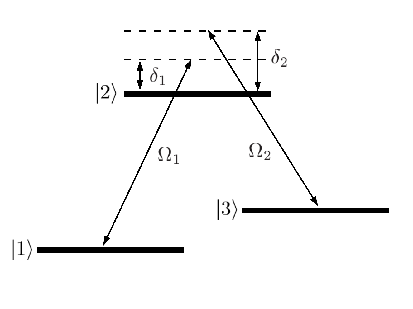
Consider a 3-level system in a -configuration (Raman 2-photon setup, Fig. 1) which is described, in a laser adapted interaction picture, by the time independent Hamiltonian () [7]
where and are the coupling strengths (Rabi frequencies) of the different transitions and and the frequency detunings as shown in Fig. 1. When the lasers are turned off (), the atomic states are uncoupled and the energy levels of cross each other at and . When the coupling lasers are turned on, these crossings become avoided crossings and transitions between the involved atomic energy levels at each resonance may occur, see Fig. 2.
An analytical diagonalization of the full Hamiltonian (II) is possible but the resulting mammoth expressions are hardly illuminating. In order to have simple formulae and gain some understanding about the different aspects of the resonances, approximations will be useful. Among the two resonances (avoided crossings) observed in the energy spectrum of the -level system we shall focus on the one at . The distance between both resonances is , and since the energy splitting of each avoided crossing is proportional to the Rabi frequencies of the coupling lasers and , the avoided crossings will be well isolated (leading to clean transitions) as long as . Under this condition, the state is scarcely populated and can be adiabatically eliminated to give an effective -level Hamiltonian as shown below.

II.1 Adiabatic elimination of state and effective Hamiltonian
Substituting the general state into the Schrödinger equation, the equations for the time dependent amplitudes are
| (5) | |||||
| (6) | |||||
| (7) |
The usual, adiabatic-elimination argument11 1 A more accurate and systematic theory, where the exact energy levels are obtained by iteration, may be used, see [4] and Appendix A. is that when , the population in level remains small, nearly zero, and thus . In this way, we may write as a function of and in the second equation and substitute in the other two,
| (8) | |||||
| (9) |
This system corresponds to an effective -level Hamiltonian
| (10) |
or, by shifting the zero of energy to make it symmetrical,
| (11) |
which corresponds to an effective coupling of a laser and a two-level system with an effective coupling strength and an effective detuning given by
| (12) | |||||
| (13) |
As described in [1], when both the diagonal and non-diagonal terms in a two-dimensional Hamiltonian depend on the same parameter ( in this simple case), the location of the resonance is not uniquely defined and it is possible to use structural and dynamical criteria to define the resonance.
II.2 Structural definition of the resonance
From the “structural” perspective of the energy-level diagram, the resonance may be defined as the point where the distance between the two branches of the avoided crossing is a minimum. The eigenenergies of are easily calculated,
| (14) |
so the minimum distance is given by the condition
| (15) |
This corresponds to a order equation, whose solution will give us the resonance position according to the structural criterion. For the condition , this is approximately given by (up to order terms in the frequencies)
| (16) |

II.3 Dynamical definition of the resonance
From a dynamical perspective the resonance is defined by the value of for which the transition probability from state to state is maximum. Using this probability is easily computed,
| (17) |
and shows a maximum at , which corresponds to
| (18) | |||||
| (19) |
This is also the middle point where the character of each dressed energy level changes, as discussed in [1]. The eigenstates of can be written as
| (20) | |||||
| (21) |
with and real Rabi frequencies , . The change of character of each dressed state is centered at the point where the linear combination has equal weights () for the states and . This occurs for an effective detuning ; i.e., this criterion coincides with the dynamical definition of the resonance.
Instead, the expressions (16) and (19) do not coincide, and are separated by a dynamical shift given in this approximation by
| (22) |
which it is plotted in Fig. 3 as a function of the ratio between the Rabi frequencies. We see a good coincidence between the exact dynamical shift and the approximation (22) for weak couplings. For strong couplings the perturbative approach breaks down, and the approximate expression deviates from the exact result. In any case, the simple form (22) still gives a good estimate of the effect.
III Experimental determination
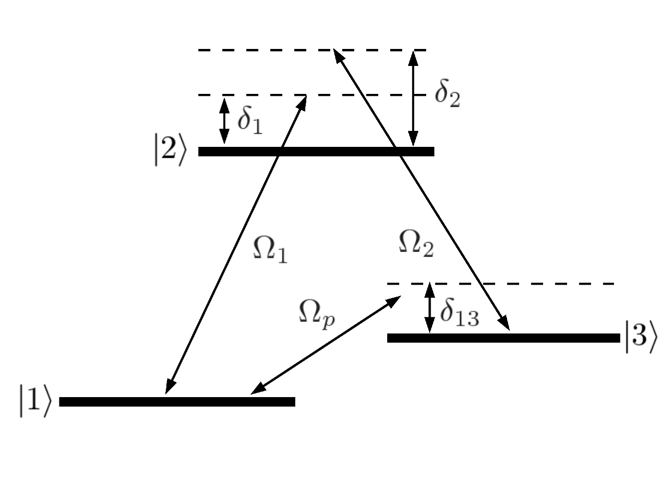
The “dynamical resonance” in Eq. (19) can be easily determined experimentally by preparing the system in state for each and looking for the maximum probability of finding state . The experimental determination of the minimum level splitting (“structural resonance”) requires some more work. One way is to use a third, auxiliary, weak probe field connecting states and as depicted in Fig. 4. This transition may be an electric-dipole forbidden transition, such as a magnetic-dipole-allowed transition. Magnetic-dipole transitions are usually much weaker than electric-dipole transitions, a good thing in this context since we are interested in probing the dressed energy levels without excessively perturbing the original system.
The Hamiltonian describing the full system (including the probe field) takes the time-dependent form
| (23) |
since, in general, there is no interaction picture in which the full Hamiltonian is time independent. Here, is the Hamiltonian of the original system already given in Eq. (II), and the time-dependent perturbation is given by
| (24) | |||||
| (25) |
being the detuning of the probe field with the transition, see Fig. 4.
We shall examine hereafter the resonance at , see Fig. 2. The dressed states will be labeled with increasing energy (), so we have to measure the energy difference between and for determining the structural resonance.
We shall now consider as a zeroth order Hamiltonian weakly perturbed by , and use (time-dependent) perturbation theory to obtain the transition rate from dressed state to dressed state ,
| (26) | |||||
with and . will show peaks at . Thus, by changing the probe detuning (sweeping the value of ) and measuring the corresponding transition rate for a fixed set of parameters of the probeless system, the energy splitting between levels and is determined. Following the same procedure for different values of , it is possible to find the minimum splitting and identify the structural resonance.

Note that the positions of the maxima of will only be located exactly at in the long time where when and the contribution of the crossed term in Eq. (26) becomes negligible. At short times, the positions of the maxima are shifted due to the dependence of the ’s, see Fig. 5a. To resolve the dynamical shift by this method, this effect should be smaller than the dynamical shift itself, which is indeed achieved at sufficiently long times, as shown in Fig. 5b.
As time increases the peaks of become narrower (the width of each peak goes like ), so in order to be able to resolve the dynamical shift, the probe beam should be applied for a time satisfying
| (27) |
In summary, for large enough times both effects (the shift due to the dependence of the ’s and the width of the peaks in order to resolve the dynamical shift) can be overcome. Note also that condition (27), which ensures narrow peaks, is more demanding than the times required to get rid of the shift due to the dependence of the ’s, see Fig. 5b.
The height of the peaks grows with time as , so to keep the perturbative treatment valid, this maximum probability has to be smaller than one (weak probe field). Combining this low probe intensity condition with the long-time condition given above, we end up with a condition for the probe-field amplitude ,
| (28) |
Actually this is just an upper bound. The exact growth of the height with time is given by , but the values of the matrix elements are bounded between and .
III.1 Discussion of specific systems
The most obvious setting for a Raman-transition experiment is driving optical stimulated Raman transitions in alkali atoms. Unfortunately, this appears to be a difficult scenario in which to study this effect. Taking 87Rb as an example, for driving stimulated Raman transitions between hyperfine ground levels, using lasers nearly resonant with the D2 line ( transition), typical parameters are a detuning GHz and Rabi frequencies MHz. These parameters give a lowest-order dynamical shift [Eq. (22)] of 400 Hz. However, with an excited-state decay rate of MHz, the rate of spontaneous scattering from the Raman fields is around , or about 3.8 kHz. The problem here is that the dressed states will be broadened at the kHz level, and the interaction time of the probe will be limited, so that the the resolution of the probe will be too poor to resolve the dynamical shift. Decreasing the scattering rate also does not help much; for example, increasing the detuning to GHz leads to a scattering rate of only 38 Hz, but a dynamical shift of only 400 mHz. The scattering rate becomes comparable to the dynamical shift for a detuning of only 1 GHz, which is realistically too small for precision measurements.
A more promising experimental realization is possible by driving microwave transitions in the hyperfine structure of the ground electronic level of atoms. Here, spontaneous emission is completely ignorable, as the magnetic-dipole transition lifetimes are much longer than any reasonable laboratory time scale. In particular, we consider here the ground state of alkali atoms, which is split into two hyperfine levels, , where is the nuclear-spin quantum number. The three hyperfine sublevels corresponding to the setup in Fig. 1 are and for the two Raman-coupled states, and for the intermediate (“excited”) state. The degeneracy of the and states is broken by applying a magnetic bias field
| (29) |
where is the zero-field hyperfine splitting, and are the electronic and nuclear -factors, respectively, and . This represents the center of an avoided crossing of the and states, and thus the splitting at this bias-field strength,
| (30) |
is insensitive to first order to bias-field fluctuations. This reduces the need for stringent experimental control over magnetic fields, and reduces the most important systematic error in measuring the Raman resonances. With the same magnetic field, the energy of the “excited” state is above that of the state by an amount
| (31) |
For example, for 87Rb, with GHz and , the bias field is kG, and the splittings are GHz for the (nominal) Raman resonance, and MHz for the driving transition. The remaining () driving transition is given by the sum of the other two transition frequencies, or GHz. Both Raman driving transitions are driven by circularly polarized fields, while the probe field is driven by linearly polarized field.
Continuing with the 87Rb example, the Raman fields may be applied with Rabi frequencies of kHz, corresponding to field intensities of about 7.6 W/cm2 on both transitions. Microwave fields of this intensity, for example, have been realized around 6.8 GHz in the near-field of an atom chip to manipulate a Bose–Einstein condensate of 87Rb [8]. Thus, a field of this strength for the GHz transition is feasible, and the field for the MHz transition should similarly pose no problem. For a Raman detuning MHz, the lowest-order dynamical shift from Eq. (22) is 2.0 kHz.
In the choice of parameters here, it is also convenient to have very different Raman transition frequencies (6.8 and 0.9 GHz for the and fields, respectively), to control the secondary ac Stark shifts that we have not explicitly accounted for. That is, for example, the 6.8 GHz field driving the transition also couples the the transition at GHz, albeit much farther off resonance. As long as is held fixed, the Stark shift of due to the field is inconsequential, as it simply causes a common shift of both structural and dynamic resonances. However, the Stark shift of due to the field depends on , and thus can cause an additional contribution to the dynamical shift . However, this effect is suppressed by the ratio of the detuning from the transition to the detuning from the transition. This effect should thus be smaller than the lowest-order shift of kHz by a factor of about , and is therefore negligible. Note also that it is important to have Raman detunings much smaller than the transition frequencies, in order to suppress the effects of Bloch–Siegert shifts. By a similar argument, the contribution of the Bloch–Siegert shifts should be of the same order as the secondary ac Stark shifts.
Note that uncertainties in the microwave frequencies are negligible on the scale of kHz, so long as the fields are derived from digital synthesizers. However, the splitting at each detuning must be determined to an accuracy finer than the kHz shift. Thus, to resolve this shift of kHz, the (6.8 GHz) probe beam should be applied for a time much longer than s [Eq. (27)], with a Rabi frequency small compared to kHz [Eq. (28)]. The probe field then requires a correspondingly much lower intensity, as compared to the Raman fields. The atoms will also need to be well-confined on ms time scales, without inducing spontaneous emission. Loading laser-cooled atoms into a dipole trap—formed by the focused light of a CO2 laser—accomplishes this confinement, with negligible perturbation to the hyperfine structure of the ground electronic state.
Care must also be taken in preparing the atoms for the probe measurement. Since the goal is to measure the splitting of the dressed states at a particular detuning, as described above, we must prepare the atoms in only one of the dressed states. This is effected, for example, by first optically pumping the atoms (in the absence of the Raman fields, and with only a small magnetic bias field of the order of mG to prevent mixing of states) into the bare state. This is accomplished by driving the optical transition with circularly polarized light, while optically depumping the ground hyperfine level. The kG field should then be turned on adiabatically to produce the correct level configuration without inducing any transitions. The Raman fields should then also be turned on adiabatically, but far from Raman resonance. They can then be adiabatically chirped to the desired Raman detuning, transferring the atoms from to . The probe field should then be activated to attempt to drive atoms to the other dressed state . Finally, the Raman fields should again be detuned and adiabatically turned off, and the magnetic field turned off adiabatically as well. The population transferred to , and thus to , is then measured by fluorescence detection of the population. Finer resolution of the Raman splitting is also possible by employing a Ramsey-interference technique, applying the probe in two pulses separated in time.
IV Summary
As discussed in [1], avoided crossing resonances between dressed energy levels are not uniquely defined. In this paper a -level atom in a configuration has been proposed as a simple physical system where the distinction between structural and dynamical aspects of a resonance could be observed. By adiabatically eliminating the third level, an effective -dimensional Hamiltonian has been obtained, from which an approximate analytical expression for the dynamical shift (between structural and dynamical resonances) has been given.
While the dynamical resonance is in principle easy to observe by measuring the maximum rate of a given atomic transition, the determination of the structural resonance is more delicate. We have proposed a method consisting of a weak probe field. In order to resolve the dynamical shift by this method, a low-intensity probe field must be applied for sufficiently long times. An ideal setting is provided by microwave transitions in the hyperfine structure of the ground state level of alkali atoms.
Acknowledgements.
We are very grateful to C. Cohen-Tannoudji for useful comments. We acknowledge support by Ministerio de Innovación y Ciencia (FIS2009-12773-C02-01), Basque Government Grant IT472-10, and National Science Foundation Grant PHY-0855412.Appendix A Resolvent method
It is possible to improve systematically the adiabatic approximation by using a more accurate method, where the energy levels are given exactly by an implicit Hamiltonian, [4, 5]. In order to use this resolvent method, we may divide the starting Hamiltonian (II) as with
The bare energy levels (eigenergies of ) corresponding to the bare states , and are given respectively by
| (40) | |||||
| (41) | |||||
| (42) |
Around , energy levels and are degenerate but will form an avoided crossing when the lasers are turned on. Around this value of , the system will be described by an implicit effective D Hamiltonian [4],
where are the matrix elements of the level shift operator ,
| (46) |
with and . The effective Hamiltonian (A) can be written in a symmetrical way by changing the zero of the energy
with
| (52) | |||||
| (53) |
Explicit expressions of the needed elements are exactly given by
| (54) | |||||
| (55) | |||||
| (56) |
where we have taken into account that , and
| (57) | |||||
| (58) |
Note that the elements of the implicit Hamiltonian depend on the eigenenergy . Thus the energy levels will be obtained by iteration. Once the energy levels are calculated (with a given precision) the different resonance loci will be calculated as described above. Choosing for the first iteration corresponds exactly to the adiabatic elimination approximation in Sec. II.
References
- [1] I. Lizuain, E. Hernández-Concepción, and J. G. Muga, Phys. Rev. A 79, 065602 (2009).
- [2] J. I. Cirac, R. Blatt, and P. Zoller, Phys. Rev. A 49, R3174 (1994).
- [3] I. Lizuain and J. G. Muga, Phys. Rev. A 75, 033613 (2007).
- [4] C. Cohen-Tannoudji, J. Dupont-Roc, and C. Fabre, J. Phys. B 6, L214 (1973).
- [5] C. Cohen-Tannoudji, J. Dupont-Roc, and G. Grynberg, Atom-Photon Interactions (Wiley, New York, 1998).
- [6] J. R. Walkup, M. Dunn, and D. K. Watson, Phys. Rev. A 58 4668 (1998).
- [7] J. G. Muga, J. Echanobe, A. del Campo, and I. Lizuain, J. Phys. B: At. Mol. Opt. Phys. 41, 175501 (2008).
- [8] P. Böhi, M. F. Riedel, J. Hoffrogge, J. Reichel, T. W. Hänsch, and P. Treutlein, Nature Physics 5, 592 (2009).