∎
Approximation Analysis of Influence Spread in Social Networks
Abstract
In recent years, study of influence propagation in social networks has gained tremendous attention. In this context, we can identify three orthogonal dimensions – the number of seed nodes activated at the beginning (known as budget), the expected number of activated nodes at the end of the propagation (known as expected spread or coverage), and the time taken for the propagation. We can constrain one or two of these and try to optimize the third. In their seminal paper, Kempe, Kleinberg and Tardos constrained the budget, left time unconstrained, and maximized the coverage: this problem is known as Influence Maximization (or MAXINF for short).
In this paper, we study alternative optimization problems which are naturally motivated by resource and time constraints on viral marketing campaigns. In the first problem, termed Minimum Target Set Selection (or MINTSS for short), a coverage threshold is given and the task is to find the minimum size seed set such that by activating it, at least nodes are eventually activated in the expected sense. This naturally captures the problem of deploying a viral campaign on a budget. In the second problem, termed MINTIME, the goal is to minimize the time in which a predefined coverage is achieved. More precisely, in MINTIME, a coverage threshold and a budget threshold are given, and the task is to find a seed set of size at most such that by activating it, at least nodes are activated in the expected sense, in the minimum possible time. This problem addresses the issue of timing when deploying viral campaigns. Both these problems are -hard, which motivates our interest in their approximation.
For MINTSS, we develop a simple greedy algorithm and show that it provides a bicriteria approximation. We also establish a generic hardness result suggesting that improving this bicriteria approximation is likely to be hard. For MINTIME, we show that even bicriteria and tricriteria approximations are hard under several conditions. We show, however, that if we allow the budget for number of seeds to be boosted by a logarithmic factor and allow the coverage to fall short, then the problem can be solved exactly in PTIME, i.e., we can achieve the required coverage within the time achieved by the optimal solution to MINTIME with budget and coverage threshold .
Finally, we establish the value of the approximation algorithms, by conducting an experimental evaluation, comparing their quality against that achieved by various heuristics.
Keywords:
Social Networks Social Influence Influence Propagation Viral Marketing Approximation Analysis MINTSS MINTIME1 Introduction
The study of how influence and information propagate in social networks has recently received a great deal of attention (Domingos and Richardson, 2001; Richardson and Domingos, 2002; Kempe et al, 2003; Kempe et al, 2005; Kimura and Saito, 2006; Goyal et al, 2008; Chen et al, 2009; Chen et al, 2010a; Chen et al, 2010b; Goyal et al, 2010; Weng et al, 2010; Bakshy et al, 2011). One of the central problems in this domain is the problem of influence maximization (Kempe et al, 2003). Consider a social network in which we have accurate estimates of influence among users. Suppose we want to launch a new product in the market by targeting a set of influential users (e.g., by offering them the product at a discounted price), with the goal of starting a word-of-mouth viral propagation, exploiting the power of social connectivity. The idea is that by observing its neighbors adopting the product, or more generally, performing an action, a user may be influenced to perform the same action, with some probability. Influence thus propagates in steps according to one of the propagation models studied in the literature, e.g., the independent cascade (IC) or the linear threshold (LT) models (Kempe et al, 2003). The propagation stops when no new user gets activated.
In this context, we can identify three main dimensions – the number of seed nodes (or users) activated at the beginning (known as the budget), the expected number of nodes that eventually get activated (known as coverage or expected spread)11 1 We use the terms coverage and expected spread interchangeably throughout the article., and the number of time steps required for the propagation. In their seminal paper Kempe, Kleinberg, and Tardos (2003) introduced the problem of Influence Maximization (MAXINF) which asks for a seed set with a budget threshold that maximizes the expected spread (time being left unconstrained). They showed that under the standard propagation models IC and LT, MAXINF is -hard, but that a simple greedy algorithm that exploits properties of the propagation function yields a -approximation, for any (as discussed in detail in Section 2).
In this paper, we explore the other dimensions of influence propagation. The problem of Minimum Target Set Selection (MINTSS) is motivated by the observation that in a viral marketing campaign, we may be interested in the smallest budget that will achieve a desired outcome. The problem can therefore be defined as follows. We are given a threshold for the expected spread and the problem is to find a seed set of minimum size such that activating the set yields an expected spread of at least .
In both MINTSS and MAXINF, the time for propagation is not considered. Indeed, with the exception of a few papers (Leskovec et al, 2007, see e.g.,), the temporal dimension of the social propagation phenomenon has been largely overlooked. This is surprising as the timeliness of a viral marketing campaign is a key ingredient for its success. Beyond viral marketing, many other applications in time-critical domains can exploit social networks as a means of communication to spread information quickly. This motivates the problem of Minimum Propagation Time (MINTIME), defined as follows: given a budget and a coverage threshold , find a seed set that satisfies the given budget and achieves the desired coverage in as little time as possible. Thus, MINTIME tries to optimize the propagation time required to achieve a desired coverage under a given budget.
1.1 Our Contributions
We now summarize the main results in this paper.
-
Firstly, we show (Section 4, Theorem 4.1) that for all instances of MINTSS where the coverage function is submodular, a simple greedy algorithm yields a bicriteria approximation: given a coverage threshold and a shortfall parameter , the greedy algorithm will produce a solution : and , where is the optimal size of a seed set whose coverage is at least . That is, the greedy solution exceeds the optimal solution in terms of size (budget) by a logarithmic factor while achieving a coverage that falls short of the required coverage by the shortfall parameter. We prove a generic hardness result (Section 4, Theorem 4.3) suggesting that improving this approximation factor is likely to be hard.
-
For MINTIME under IC and LT model (or any model with monotone submodular coverage functions), we show that when we allow the coverage achieved to fall short of the threshold and the budget for number of seed nodes to be overrun by a logarithmic factor, then we can achieve the required coverage in the minimum possible propagation time, i.e., in the time achieved by the optimal solution to MINTIME with budget threshold and coverage threshold (Section 5, Theorem 5.3).
-
On the other hand, for MINTIME under the IC model, we show that even bicriteria and tricriteria approximations are hard. More precisely, let be the optimal propagation time required for achieving a coverage within a budget of . Then we show the following (Section 5, Theorem 5.1): there is unlikely to be a PTIME algorithm that finds a seed set with size under the budget, which achieves a coverage better than . Similarly, if we limit the budget overrun factor to less than , then it is unlikely that there is a PTIME algorithm that finds a seed set of size within the overrun budget which achieves a coverage better than . In both cases, the result holds even when we permit any amount of slack in the resulting propagation time.
-
The above results are bicriteria bounds, in that they allow slack in two of the three parameters governing MINTIME problems. We also show a tricriteria hardness result (Section 5, Theorem 5.2). Namely, if we limit the budget overrun factor to be , then it is unlikely that there is a PTIME algorithm that finds a seed set with a size within a factor of the budget that achieves a coverage better than . Similar bounds hold if we place hard limits on the coverage approximation and try to balance overrun in the other parameters.
-
Often, the coverage function can be hard to compute exactly. This is the case for both IC and LT models (Kempe, Kleinberg, and Tardos, 2003). All our results are robust in that they carry over even when only estimates of the coverage function are available.
-
We show the value of our approximation algorithms by experimentally comparing their quality with that of several heuristics proposed in other contexts, using two real data sets. We discuss our findings in Section 6.
2 Preliminaries
Suppose we are given a social network together with the estimates of mutual influence between individuals in the network, and suppose that we want to push a new product in the market. The mining problem of influence maximization is the following: given such a network with influence estimates, how to select the set of initial users so that they eventually influence the largest number of users in the social network. This problem has received a good deal of attention in the data mining and the theoretical computer science communities in the last decade.
The first to consider the propagation of influence and the problem of identification of influential users from a data mining perspective are Domingos and Richardson (2001); Richardson and Domingos (2002). The problem is modelled by means of Markov random fields and heuristics are given for choosing the users to target. In particular, the marketing objective function to maximize is the global expected lift in profit, that is, intuitively, the difference between the expected profit obtained by employing a marketing strategy and the expected profit obtained using no marketing at all. A Markov random field, is an undirected graphical model representing the joint distribution over a set of random variables, where nodes are variables, and edges represent dependencies between variables. It is adopted in the context of influence propagation by modelling only the final state of the network at convergence as one large global set of interdependent random variables.
Kempe et al (2003) tackle roughly the same problem as a problem in discrete optimization. They obtain provable approximation guarantees under various propagation models studied in mathematical sociology, as we describe next.
A social network can be represented as a directed graph . Every node is in one of two states – active or inactive. Here, “active” may correspond to a user buying a product or getting infected. In progressive models, it is assumed once a node becomes active, it remains active. Influence is assumed to propagate from nodes to their neighbors according to a propagation model, and a node’s tendency to become active increases monotonically as more of its neighbors become active.
In the independent cascade (IC) model, each active neighbor of a node has one shot at influencing and succeeds with probability , the probability with which influences . In the linear threshold (LT) model, each node is influenced by each neighbor according to a weight , such that the sum of incoming weights to is no larger than . Each node chooses a threshold uniformly at random from the interval . If at timestamp , the total weight from the active neighbors of attains the threshold , then will become active at timestamp . In both the models, the process repeats until no new node becomes active.
For any propagation model, the expected influence spread of a seed set is the expected number of nodes that eventually get activated by initially activating the nodes . We denote this number by , where stands for the underlying propagation model. Then the influence maximization problem is defined as follows. Given a directed and edge-weighted social graph , a propagation model , and a number , find a set , , such that is maximum.
Under both the IC and LT propagation models, this problem is shown to be -hard (Kempe et al, 2003). However, for both the propagation models described above, the expected influence spread function is monotone and submodular. Monotonicity says as the set of activated nodes grows, the likelihood of a node getting activated should not decrease. More precisely, a A function from sets to reals is monotone if whenever . A function is submodular if . Submodularity intuitively says an active node’s probability of activating some inactive node does not increase if more nodes have already attempted to activate and is hence more “marketing-saturated”. It is also called the law of “diminishing returns”.22 2 A variant of the linear threshold model, where a deterministic threshold is chosen for each node, has also been studied (Chen, 2008; Ben-Zwi et al, 2009). Coverage under this variant is not submodular.
Thanks to these two properties we can have a simple greedy algorithm (see Algorithm 1) for infuence maximization which provides an approximation guarantee. In fact, for any monotone submodular function with , the problem of finding a set of size such that is maximum, can be approximated to within a factor of by the greedy algorithm Nemhauser et al (1978). This result carries over to the influence maximization problem Kempe et al (2003), meaning that the seed set we produce using Algorithm 1 is guaranteed to have an expected spread i.e., , of the expected spread of the optimal seed set.
The complex step of the greedy algorithm is in line 3, where we select the node that provides the largest marginal gain with respect to the expected spread of the current seed set . Computing the expected spread given a seed set is -hard under both the IC model (Chen et al, 2010a) and the LT model (Chen et al, 2010b). In their paper, Kempe et al. run Monte Carlo (MC) simulations of the propagation model for sufficiently many times (the authors report trials) to obtain an accurate estimate of the expected spread, resulting in a very long computation time. In particular, they show that for any , there is a such that by using -approximate values of the expected spread, we can obtain a -approximation for the influence maximization problem.
We now define the problems we study in this paper. Let stand for any propagation model with a submodular coverage function .
Problem 1 (MINTSS)
Let be a social graph. Given a real number , find a set of the smallest size , such that the expected spread, denoted , is no less than .
Problem 2 (MINTIME)
Let be a social graph. Given an integer , and a real number , find a set , , and the smallest , such that the expected spread at time , denoted , is no less than .
The MINTSS problem is closely related to the real-valued submodular set cover (RSSC) problem, defined as follows: given a submodular function and a threshold , find a set of the least size (or minimum cost, when elements of are weighted) such that . MINTSS under any propagation model such as IC and LT, for which the coverage function is submodular is clearly a special case of RSSC, an observation we exploit in Section 4.
MINTIME is closely related to the Robust Asymmetric -center (RAKC) problem in directed graphs, defined as follows: given a digraph , a (possibly empty) set of forbidden nodes and thresholds and , find or fewer nodes such that they cover at least non-forbidden nodes in the minimum possible radius, i.e., each of the nodes are reachable from some node in in the minimum possible distance.
3 Related Work
While to the best of our knowledge, MINTIME has never been studied before, some work has been devoted to MINTSS. Chen (2008) shows that under the LT propagation model with fixed (and hence deterministic) thresholds, MINTSS cannot be approximated within a factor of unless , and also gives a polynomial time algorithm for MINTSS on trees. Coverage under the LT model with deterministic thresholds is not submodular.
Ben-Zwi et al (2009) build upon Chen (2008) and develop a algorithm for solving MINTSS exactly under the deterministic linear threshold model, where is the tree width of the graph. They show the problem cannot be solved in time unless all problems in SNP can be solved in sub-exponential time. In this paper, we study both MINTSS and MINTIME under the classic propagation models, under which the coverage function is submodular.
A few classical cover-problems are related to the problems we study. One such problem is Maximum Coverage (MC): given a collection of sets over a ground set and budget , find a subcollection such that and is maximized. The problem can be approximated within a factor of and it cannot be improved (Feige, 1998; Khuller et al, 1999). Similar results by Khuller et al (1999) and Sviridenko (2004) exist for the weighted case.
Another relevant problem is Partial Set Cover (PSC): given a collection of sets over the ground set and a threshold , the goal is to find a subcollection such that and is minimized. While PSC can be approximated within a factor of , Feige (1998) showed that it cannot be approximated within a factor of , for any fixed , unless .
Our results on MINTSS exploit its connection to the real-valued submodular set cover (RSSC) problem. There has been substantial work on submodular set cover (SSC) in the presence of integer-valued submodular functions, which is a generalization of the classical Set Cover Problem (Fujito, 1999; Fujito, 2000; Feige, 1998; Slavík, 1997; Bar-Ilan et al, 2001). Relatively much less work has been done on real-valued SSC. For non-decreasing real-valued submodular functions, Wolsey (1982) has shown, among other things, that a simple greedy algorithm yields a solution to a special case of SSC where , that is within a factor of of the optimal solution, where is the number of iterations needed by the greedy algorithm to achieve a coverage of and denotes the greedy solution after iterations. Unfortunately, this result by itself does not yield an approximation algorithm with any guaranteed bounds: in Appendix B we give an example to show that the greedy solution can be arbitrarily worse than the optimal one. Furthermore, Wolsey’s analysis is restricted to the case . Along the way to establishing our results on MINTSS, we show the greedy algorithm yields a bicriteria approximation for real-valued SSC that extends to the general case of partial cover with , and where elements are weighted.
Our results on MINTIME leverage its connection to the robust asymmetric -center problem (RAKC). It has been shown that, while asymmetric -center problem can be approximated within a factor of (Panigrahy and Vishwanathan, 1998), RAKC cannot be approximated within any factor unless P = NP (Li Gørtz and Wirth, 2006).
4 Minimum Target Set Selection
4.1 A Bicriteria Approximation
Our main result of this section is that a simple greedy algorithm, Algorithm Greedy-Mintss, yields a bicriteria approximation to (weighted) MINTSS, for any propagation model whose coverage function is monotone and submodular.
In order to prove the results in the most general setting, we consider digraphs which have non-negative node weights: we are given a cost function in addition to the coverage threshold , and need to find a seed set such that and is minimum. Clearly, this generalizes the unweighted case.
Theorem 4.1
Let be a social graph, with node weights given by . Let be any propagation model whose coverage function is monotone and submodular. Let be a seed set of minimum cost such that . Let be any shortfall and let be the greedy solution with chosen threshold . Then, .
In the rest of this section, we prove this result. We first observe that every instance of MINTSS where the coverage function is monotone and submodular is an instance of RSSC. Thus, it suffices to prove Theorem 4.1 for RSSC, for which we adapt a bicriterion approximation technique by Slavík (1997).
Let be a ground set, be a cost function, a non-negative monotone submodular function and a given threshold. Apply the greedy algorithm above to this instance of RSSC. Let be the (partial) solution obtained by the greedy algorithm after iterations. Let be the smallest number such that . We define . Clearly, is also monotone and submodular. In each iteration, the greedy algorithm picks an element which provides the maximum marginal gain per unit cost (w.r.t. ), i.e., it picks an element for which is positive and is maximum.
Let and define , i.e., the shortfall in coverage after iterations of the greedy algorithm.
Lemma 1
At the end of iteration , there is an element : .
Proof. Let . Let and . Suppose . Consider adding the elements in to one by one. Clearly, at any step , we have by submodularity that
Iterating over all , this yields resulting in which is a contradiction since the left hand side is no less than the optimal coverage. ∎
Proof of Theorem 4.1:
It follows from Lemma 1 that where is the cost of the element added in iteration . Using the well known inequality , we get . Expanding, . Let the algorithm take iterations to achieve coverage such that . At any step, . Thus, , and in particular, the cost of the last element picked can be at most . So, . implies . Hence, we have which implies . Thus, . ∎
Using a similar analysis, it can be shown that when the costs are uniform, the approximation factor can be improved to .
For propagation models like IC and LT, computing the coverage exactly is -hard (Chen et al, 2010a; Chen et al, 2010b) and thus we must settle for estimates. To address this, we “lift” the above theorem to the case where only estimates of the function are available. We can show:
Theorem 4.2
For any , there exists a such that using ()-approximate values for the coverage function , the greedy algorithm approximates MINTSS under IC and LT models within a factor of .
Proof. The proof involves a more careful analysis of how error propagates in the greedy algorithm if, because of errors, the greedy algorithm picks the wrong point.
Here, we give the proof for the unit cost version only. Consider any monotone, submodular function . Thus, in the statement of theorem, . Let be its approximated value. In any iteration, the (standard) greedy algorithm picks an element which provides maximum marginal gain. Let be the set formed after iteration .
As we did in Lemma 1, it is straightforward to show that there must exists an element such that where . Without loss of generality, let be the element which provides the maximum marginal gain. Suppose that due to the error in computing , some other element is picked instead. Then,
Moreover, . Thus,
Let . Let the greedy algorithm takes iterations. Then,
Using and ,
The algorithm stops when . The maximum number of iterations needed to ensure this are
Let . To prove the lemma, we need to prove that for any , there exists such that
Clearly, for any , . Hence,
This completes the proof for unit cost case. Using the slight modification in the greedy algorithm (as we did in proving theorem 1), the same result can be obtained for weighted version. ∎
4.2 An Inapproximability Result
Recall that every instance of MINTSS where the coverage function is monotone and submodular is an instance of RSSC. Consider the unweighted version of the RSSC problem. Let denote an optimal solution and let .
Theorem 4.3
For any fixed , there does not exist a PTIME algorithm for RSSC that guarantees a solution , and for any unless .
Proof. Case 1: . Suppose there exists an algorithm that finds a solution of size such that for any . Consider an arbitrary instance of PSC, which is a special case of RSSC. Apply the algorithm to . It outputs a collection of sets that covers elements in .
Create a new instance of PSC as follows. Let be the set of elements of covered by . Define , and . Set the new shortfall . Apply the algorithm to . It will output another collection of sets which covers elements in .33 3 If , outputs an empty collection. Let . The number of elements covered by is . Clearly, . Thus, we have a solution for PSC with the approximation factor of , which is not possible unless (Feige, 1998). This proves Case 1.
Case 2: . Assume an arbitrary instance of RSSC with monotone submodular function . Let be the coverage threshold and be any given shortfall. We now construct another instance of RSSC as follows: Set the coverage function , coverage threshold and shortfall . Choose any value of such that . We now show that if a solution is a -approximation to the optimal solution for then it is a -approximation to the optimal solution for . Clearly, the optimal solution for both the instances are identical, so .44 4 Here, and represent the size of the optimal solution for instances and respectively. Suppose there exists an algorithm for RSSC when the shortfall is , that guarantees a solution and . Apply this algorithm to instance to obtain a solution . We have: . It implies . Moreover, , implying . Thus we have the solution for instance whose size is . The theorem follows. ∎
In view of this generic result, we conjecture that improving the approximation factor for MINTSS to for IC and LT is likely to be hard.
5 MINTIME
In this section, we study MINTIME under the IC model. Denote by the expected number of nodes activated under model within time , and let be the desired coverage and be the desired budget. Let denote the optimal propagation time under these budget and coverage constraints. Our first result says that efficient approximation algorithms are unlikely to exist under two scenarios: (i) when we allow a coverage shortfall of less than and (ii) when we allow a budget overrun less than . In the former scenario, we have a strict budget threshold and in the latter we have a strict coverage threshold. In both cases, we allow any amount of slack in propagation time.
Theorem 5.1
Unless , there does not exist a PTIME algorithm for MINTIME that guarantees (for any ):
- 1.
a ()-approximation, such that , and where for any fixed ; or
- 2.
a ()-approximation, such that , and where for any fixed .
Our second theorem says efficient approximation algorithms are unlikely to exist under more liberal scenarios than those given above: (i) when for a given budget overrun factor , the fraction of the coverage we want to achieve is more than and (ii) when for a given fraction of the coverage we want to achieve, the budget overrun factor we allow is less than . As before, we allow any amount of slack in propagation time.
Theorem 5.2
Unless there does not exist a PTIME algorithm for MINTIME that guarantees ()-approximation factor (for any ) such that , and where
- 1.
and for any fixed ; or
- 2.
and for any fixed .
Finally, on the positive side, we show that when a coverage shortfall of is allowed and a budget boost of is allowed, we can in PTIME find a solution which achieves the relaxed coverage under the relaxed budget in optimal propagation time. More precisely, we have:
Theorem 5.3
Let the chosen coverage threshold be , for and chosen budget threshold be . If the coverage function can be computed exactly, then there is a greedy algorithm that approximates the MINTIME problem within a ( factor where , and for any . Furthermore, for every , there is a such that by using a -approximate values for the coverage function , the greedy algorithm approximates the MINTIME problem within a ( factor where , and .
5.1 Inapproximability Proofs
We next prove Theorems 5.1 and 5.2. We first show that MINTIME under the IC model generalizes the RAKC problem. In a digraph and sets of nodes , say that -covers if for every , there is a such that there is a path of length from to . Given an instance of RAKC, create an instance of MINTIME by labeling each arc in the digraph with a probability . Now, it is easy to see that for any set of nodes and any , -covers a set of nodes iff activating the seed nodes will result in the set of nodes being activated within time steps. Notice that since all the arcs are labeled with probability , all influence attempts are successful by construction. It follows that RAKC is a special case of MINTIME under the IC model.
The tricriteria inapproximability results of Theorem 5.2 subsume the bicriteria inapproximability results of Theorem 5.1. Still, in our presentation, we find it convenient to develop the proofs first for bicriteria. Since we showed that MINTIME under IC generalizes RAKC, it suffices to prove the theorems in the context of RAKC. It is worth pointing out Li Gørtz and Wirth (2006) proved that it is hard to approximate within any factor unless . Their proof only applies to (the standard) unicriterion approximation.
For a set of nodes in a digraph we denote by the number of nodes that are -covered by . Recall the problems MC and PSC (see Section 3).
Proof of Theorem 5.1: It suffices to prove the theorem for RAKC. For claim 1, we reduce Maximum Coverage (MC) to RAKC and for claim 2, we reduce PSC to RAKC. The reduction is similar and is as follows: Consider an instance of the decision version of MC (equivalently PSC) , where we ask whether there exists a subcollection of size such that . Construct an instance of RAKC as follows: the graph consists of two classes of nodes – and . For each , create a class A node and for each , create a class B node . There is a directed edge of unit length iff . Notice, a set of nodes in -covers another non-empty set of nodes iff -covers the latter set. Moreover, sets in cover elements in iff has a set of nodes which -covers nodes. The only-if direction is trivial. For the if direction, the only way nodes can -covers nodes in is when the nodes are from class A.
Next, we prove the first claim. Set and . Assume there exists a PTIME (, )-approximation algorithm for RAKC such that for any fixed , for some . Apply algorithm to the instance . Notice, for our instance, . The coverage by the output seed set will be nodes, for some , implying that the number of class B nodes covered is . Thus the algorithm approximates MC within a factor of . Let . If we show , we are done, since MC cannot be approximated within a factor of for any unless (Feige, 1998; Khuller et al, 1999). Clearly, is not always positive. However, for a given and , is an increasing function of and reaches in the limit. Hence there is a value , . That is, there are infinitely many instances of PSC for which is a -approximation algorithm, where , which proves the first claim.
Next, we prove the second claim. Set and . The value of will be decided later. Assume there exists a PTIME (, )-approximation algorithm for RAKC where for any fixed . Apply the algorithm to . It gives a solution such that that covers nodes. A difficulty arises here since can be arbitrarily close to making arbitrarily small, for any given and . However, as we argued in the proof of claim 1, for sufficiently large , we can always find an : . That is, on infinitely many instances of PSC, algorithm finds a set of class A nodes which -covers nodes, for some . Without loss of generality, we can assume . Choose the smallest value of such that the solution covers class B nodes. This implies the number of class A nodes covered is and so . Thus, on all such instances, algorithm gives a solution of size : that covers nodes. If we show that the upper bound is equal to for some , we are done, since PSC cannot be approximated within a factor of unless (Feige, 1998).
Let , which yields . It is easy to see that by choosing sufficiently large , we can make the gap between and arbitrarily small and thus can always ensure on infinitely many instances of PSC, on each of which algorithm will serve as an -approximation algorithm proving claim . ∎
Note, in the proofs of both claim and in the above theorem, by choosing sufficiently large, we can always ensure for any given and , the corresponding is always greater than . To prove the tricriteria hardness results, we need the following lemma.
Lemma 2
In the MC (or PSC) problem, let be the minimum number of sets needed to cover elements. Then, unless , there does not exist a PTIME algorithm that is guaranteed to select sets covering elements where
- 1.
and ; or
- 2.
and for any fixed .
Proof of Theorem 5.2: Again, it suffices to prove the theorem for RAKC. For claim 1, we reduce MC to RAKC and for claim 2, we reduce PSC to RAKC. The reduction is the same as in the proof of Theorem 5.1 and we skip the details here. Below, we refer to instances and as in that proof.
We first prove claim 1. Given any , set and . Assume there exists a PTIME (, , )-approximation algorithm for RAKC which approximates the problem within the factors as mentioned in claim 1. Apply algorithm to the instance . The coverage by the output seed set will be nodes, implying the number of class B nodes covered is . Thus the algorithm approximates MC within a factor of .
If we show , then the claim follows, since MC cannot be approximated within a factor of for any unless , by Lemma 2. Let . For any , is an increasing function of which approaches in the limit. Thus, given any fixed , there must exist some such that for any , . This proves the first claim (by an argument similar to that in Theorem 5.1).
Next, we prove the second claim. Set and . The value of will be decided later. Assume that there exists a PTIME (, , )-approximation algorithm for RAKC where the factors , and satisfy the conditions as mentioned in claim 2. Apply the algorithm to instance . For any , it gives a solution of size that covers nodes. There can be possible choices of . Pick the smallest such that number of nodes covered in class B is at least , implying that the number of nodes picked from class A is . Thus, . The existence of satisfying this inequality can be established as done for claim 2 in Theorem 5.1.
Thus, algorithm gives the solution instance of size that covers elements in where . If we show that for any given and in the range, there exists some and such that and , then the claim follows. Let , then .
Whenever , we can always choose such that . The non-trivial case is when . In this case, by choosing a large enough , we can make arbitrarily close to and make . In other words, there exists some : for all , , and by an argument similar to that for claim 2 in Theorem 5.1, the claim follows. ∎
5.2 A Tri-criteria Approximation
We now consider upper bounds for MINTIME. It is interesting to ask what happens when either the budget overrun or the coverage shortfall is increased. We show that under these conditions, a greedy strategy combined with linear search yields a solution with optimal propagation time. This proves Theorem 5.3.
Algorithm Greedy-Mintss computes a small seed set that achieves coverage . Recall that denotes the coverage of under propagation model within time steps. It is easy to see that Greedy-Mintss can be adapted to instead compute a seed set that yields coverage within time steps: we call this algorithm Greedy-MintssR.
Given such an algorithm, a simple linear search over yields the bounds specified in Theorem 5.3, after setting coverage threshold as and the chosen budget threshold as . The approximation factors in the theorem follow from Theorem 4.1 and Lemma 4.2. These bounds continue to hold if we can only provide estimates for the coverage function (rather than computing it exactly) and also extend to weighted nodes.
We conclude this section by noting that the algorithm above can be naturally adapted to the RAKC problem. The bounds in Theorem 5.3 apply to RAKC as well, since MINTIME under IC generalizes RAKC.
6 Empirical Assessment
We conducted several experiments to assess the value of the approximation algorithms by comparing their quality against that achieved by several well-known heuristics, as well as against the state-of-the-art methods developed for MAXINF that we adapt in order to deal with MINTSS and MINTIME. In particular, the goals of experimental evaluation are two-fold. First, we have previously established from theoretical analysis that the Greedy algorithm (Greedy-Mintss for MINTSS and Greedy-MintssR for MINTIME) provides the best possible solution that can be obtained in PTIME, which we would like to validate empirically. Second, we study the gap between the solutions obtained from various heuristics against the Greedy algorithm, the upper bound, in terms of quality.
In what follows we assume the IC propagation model.
Datasets, probabilities and methods used. We use two real-world networks, whose statistics are reported in Table 1.
The first network, called NetHEPT, is the same used in Chen et al (2009); Chen et al (2010a); Chen et al (2010b). It is an academic collaboration network extracted from ‘‘High Energy Physics - Theory’’ section of arXiv55 5 http://www.arXiv.org, with nodes representing authors and edges representing coauthorship. This is clearly an undirected graph, but we consider it directed by taking for each edge the arcs in both the directions. Following Kempe et al (2003); Chen et al (2009); Chen et al (2010a), we assign probabilities to the arcs in two different ways: uniform, where each arc has probability 0.1 (or probability 0.01) and weighted cascade (WC), i.e, the probability of an arc is , where indicates in-degree (Kempe et al, 2003). Note that WC is a special case of IC where probabilities on arcs are not necessarily uniform.
| NetHEPT | Meme | |
| 15233 | 7418 | |
| 62794 | 39170 | |
| 4.12 | 5.28 | |
| (strong) | 1781 | 4552 |
| (strong) | 6794 (44.601%) | 2851 (38.434%) |
| clustering coefficient | 0.31372 | 0.06763 |
| Random | Simply add nodes at random to the seed set, |
|---|---|
| until the stopping condition is met. | |
| High Degree | Greedily add the highest degree node to the |
| seed set, until the stopping condition is met. | |
| Page Rank | The popular index of nodes’ importance. |
| We run it with the same setting used | |
| in Chen et al (2010a). | |
| Sp | The shortest-path based heuristic for the |
| greedy algorithm introduced in | |
| Kimura and Saito (2006). | |
| Pmia | The maximum influence arborescence |
| method of Chen et al (2010a) with | |
| parameter . | |
| Greedy | Algorithm Greedy-Mintss for MINTSS |
| and Algorithm for | |
| MINTIME. |
The second one, called Meme, is a sample of the social network underlying the Yahoo! Meme66 6 http://meme.yahoo.com/ microblogging platform. Nodes are users, and directed arcs from a node to a node indicate that “follows” . For this dataset, we also have the log of posts propagations during 2009. We sampled a connected sub-graph of the social network containing the users that participated in the most re-posted items. The availability of posts propagations is significant since it allows us to directly estimate actual influence.
 |
 |
 |
| (a) NetHEPT- WC | (b) NetHEPT- uniform | (c) Meme |
In particular, here a propagation is defined based on reposts: a user posts a meme, and if other users like it, they repost it, thus creating cascades. For each meme and for each user , we know exactly from which other user she reposted, that is we have a relation where is the time at which the repost occurs, and is the user from which the information flowed to user . The maximum likelihood estimator of the probability of influence corresponding to an arc is where denotes the number of memes that posted before , and denotes the number of memes such that .
For the sake of comparison, we adapt the state-of-the-art methods developed for MAXINF (also see Section 3) to deal with MINTSS and MINTIME. For most of the techniques the adaptation is straightforward. The methods that we use in the experimentation are succinctly summarized in Table 2. It is noteworthy that PMIA is one of the state-of-the-art heuristic algorithms proposed for MAXINF under the IC model by Chen et al (2010a). In all our experiments, we run 10,000 Monte Carlo simulations for estimating coverage.
MINTSS - Our experimental results on the MINTSS problem are reported in Figure 1. In each of the three plots, we report, for a given coverage threshold (-axis), the minimum size of a seed-set (budget, reported on -axis) achieving such coverage. As Greedy provides the upper bound on the quality that can be achieved in PTIME, in all the experiments it outperforms the other methods, with Random and High Degree consistently performing the worst.
We analyzed the probability distributions of the various data sets we experimented with. At one extreme is the model with uniformly low probabilities (0.01). In Meme, about 80% of the probabilities are . In NetHEPT WC, on the other hand, approximately 83% of the probabilities are and about 66% of the probabilities are . However, the combination of a power law distribution of node degrees in NetHEPT together with assignment of low probabilities for high degree nodes (since it’s the reciprocal of in-degree) has the effect of rendering central nodes act as poor influence spreaders. And the arcs with high influence probability are precisely those that are incident to nodes with a very low degree. This makes for a low influence graph overall, i.e., propagation of influence is limited. Finally, at the other extreme is the model with uniformly high probabilities (0.1) which corresponds to a high influence graph.
We tested uniformly low probabilities (0.01), and we observed that with such low probabilities, there is limited propagation happening: for instance, in order to achieve a coverage of 150, even the best method requires more than 100 seeds. This forces the quality of all algorithms to look similar.
 |
 |
 |
| (a) NetHEPT- WC, Budget=75 | (b) NetHEPT- Uniform, Budget=75 | (c) Meme, Budget=150 |
 |
 |
 |
| (a) NetHEPT- WC, =1000 | (b) NetHEPT- Uniform, =1000 | (c) Meme, =1000 |
On data sets where there is a non-uniform mix of low and high probabilities, but the probabilities being predominantly low, as well as on data sets corresponding to low influence graphs, the Pmia method of Chen et al (2010a) and the Sp method of Kimura and Saito (2006), originally developed as efficient heuristics for the MAXINF problem, when adapted to the MINTSS problem, continue to provide a good approximation of the results achieved by the Greedy algorithm (Figure 1(a), (c)). In these situations, the Random and HighDegree heuristics provide seed sets much larger than Greedy. In NetHEPT WC (Figure 1(a)), PageRank has a performance that is close to the Greedy solution, while in Meme(Figure 1(c)), the seed set generated by PageRank is much larger than Greedy. In data sets with uniformly high probabilities (0.1), the gap between between Greedy and other heuristics is substantial (Figure 1(b)). Greedy can achieve a target coverage , with just seeds, while Pmia and Sp need and seeds respectively; similarly Greedy can achieve a target coverage , with just seeds, while Pmia and Sp need and seeds respectively. It is worth noting that Random, HighDegree, and the PageRank heuristic all generate seed sets much larger than Greedy on this data set. To sum, the gap between the sizes of the seed sets obtained by the heuristics one the one hand and the Greedy algorithm on the other, varies depending on the influence probabilities on the edges. In general, on graphs with high influence, the gap can be substantial.
MINTIME - Our experimental results on the MINTIME problem are reported in Figures 2 and 3. In Figure 2, we report, for a coverage threshold given on the -axis, and a fixed budget (75 for NetHEPT, 150 for Meme), the minimum time steps needed to achieve such coverage with the given budget (-axis). As expected, Greedy outperforms all the heuristics. All the plots show that after a certain time, there is no further gain in the coverage, indicating the influence decays over time. Figure 2(a) compares the various heuristics with the Greedy on the NetHEPT dataset under WC model. On this data set, Pmia, Sp and Greedy exhibit comparable performance. The Pagerank heuristic comes close to them.
Figure 2(b) shows the results for the NetHEPT dataset under IC model with uniform probability 0.1. Here, Greedy outperforms all the other heuristics. For instance, when coverage threshold is 900 and budget is 75, Greedy achieves the coverage in 5 time steps, and Sp in 6 time steps, Pmia in 14 time steps. Random, High Degree and Pagerank fail to find a solution. Similarly, when coverage threshold is 1000 and budget is 75, Greedy achieves the coverage in 6 steps whereas all other heuristics fail to find a solution with this coverage.
Finally, Figure 2(c) shows the results on Meme dataset. As we increase the target coverage, the other heuristics fail to give a solution, one by one. Beyond , all but Sp, and Pmia fail and beyond , all but Pmia fail. On this data set, Pmia provides a good approximation to the performance of Greedy.
In Figure 3, we fix the coverage threshold ( for all the plots). The plots show the minimum time steps needed to achieve the coverage w.r.t. different seed set sizes (budget). In all the cases, Random fails to find a solution and hence is not shown in the plots. The performance of the High Degree algorithm is poor as well and it fails to find a solution in case of NetHEPT with uniform probabilities 0.1. As expected, Greedy outperforms all the heuristics and provides us the lower bound on time needed to achieve the required coverage with a given budget.
Overall, we notice that the performance quality of all other heuristics compared to Greedy follows a similar pattern to that observed in case of MINTSS: as the graph changes from a low influence graph to a high influence graph, the heuristics’ performance drops substantially compared to Greedy.
Another key takeaway from the MINTIME plots is the following. For a given budget, as observed above, the choice of the seed set plays a key role in determining whether a given coverage threshold can be reached or not, no matter how much time we allow for the influence to propagate. Even if the given coverage threshold is achieved, the choice of the seed set can make a big difference to the number of time steps in which the coverage threshold is reached. Often, for a given budget, relaxing the coverage threshold can dramatically change the propagation time. E.g., In Figure 2(a) (budget fixed to 75), while Greedy takes 8 time steps to achieve a coverage of 1200, when we relax the threshold to 1100, the propagation time decreases by %, that is, to just 4 time steps. A similar phenomenon is observed when the budget is boosted w.r.t. a fixed coverage threshold. For instance, in Figure 3(c), while using 15 seeds, Greedy takes 6 time steps to achieve a coverage of 1000, it achieves the same coverage by seeds in % of the time, that is, in 2 time steps. These findings further highlight the importance of the MINTIME problem.
7 Conclusions
In this paper, we study two optimization problems in social influence propagation: MINTSS and MINTIME. We present a bicriteria approximation for MINTSS which delivers a seed set larger than the optimal seed set by a logarithmic factor , that achieves a coverage of , which falls short of the coverage threshold by . We also show a generic tightness result that indicates improving the above approximation factor is likely to be hard.
Turning to MINTIME, we give a greedy algorithm that provides a tricriteria approximation when allowed a budget overrun by a factor of and a coverage shortfall by , and achieves the optimal propagation time under these conditions. We also provide hardness results for this problem. We conduct experiments on two real-world networks to compare the quality of various popular heuristics proposed in a different context (with necessary adaptations) with that the greedy approximation algorithms. Our results show that the greedy algorithms outperform the other methods in all the settings (as expected) but depending on the characteristics of the data, some of the heuristics perform competitively. These include the recently proposed heuristics Pmia Chen et al (2010a) and Sp Kimura and Saito (2006) which we adapted to MINTSS and MINTIME.
Several questions remain open, including proving optimal approximation bounds for MINTSS and MINTIME, as well as complexity results for these problems under other propagation models.
References
- Bakshy et al (2011) Bakshy E, Hofman JM, Mason WA, Watts DJ (2011) Everyone’s an influencer: quantifying influence on twitter. In: Proceedings of the fourth ACM international conference on Web search and data mining, ACM, New York, NY, USA, WSDM ’11, pp 65–74
- Bar-Ilan et al (2001) Bar-Ilan J, Kortsarz G, Peleg D (2001) Generalized submodular cover problems and applications. Theoretical Computer Science 250(1-2):179 – 200
- Ben-Zwi et al (2009) Ben-Zwi O, Hermelin D, Lokshtanov D, Newman I (2009) An exact almost optimal algorithm for target set selection in social networks. In: EC ’09: Proceedings of the tenth ACM conference on Electronic commerce, ACM, New York, NY, USA, pp 355–362
- Chen (2008) Chen N (2008) On the approximability of influence in social networks. In: SODA ’08: Proceedings of the nineteenth annual ACM-SIAM symposium on Discrete algorithms, Society for Industrial and Applied Mathematics, Philadelphia, PA, USA, pp 1029–1037
- Chen et al (2009) Chen W, Wang Y, Yang S (2009) Efficient influence maximization in social networks. In: Proc. of the 15th ACM SIGKDD Int. Conf. on Knowledge Discovery and Data Mining (KDD’09)
- Chen et al (2010a) Chen W, Wang C, Wang Y (2010a) Scalable influence maximization for prevalent viral marketing in large-scale social networks. In: Proc. of the 16th ACM SIGKDD Int. Conf. on Knowledge Discovery and Data Mining (KDD’10)
- Chen et al (2010b) Chen W, Yuan Y, Zhang L (2010b) Scalable influence maximization in social networks under the linear threshold model. In: Proceedings of the 10th IEEE International Conference on Data Mining (ICDM’2010)
- Domingos and Richardson (2001) Domingos P, Richardson M (2001) Mining the network value of customers. In: Proceedings of the seventh ACM SIGKDD international conference on Knowledge discovery and data mining, ACM, New York, NY, USA, KDD ’01, pp 57–66
- Feige (1998) Feige U (1998) A threshold of for approximating set cover. J ACM 45(4):634–652
- Fujito (1999) Fujito T (1999) On approximation of the submodular set cover problem. Operations Research Letters 25(4):169 – 174
- Fujito (2000) Fujito T (2000) Approximation algorithms for submodular set cover with applications. IEICE Trans Inf Syst 83
- Goyal et al (2008) Goyal A, Bonchi F, Lakshmanan LV (2008) Discovering leaders from community actions. In: Proceeding of the 17th ACM conference on Information and knowledge management, ACM, New York, NY, USA, CIKM ’08, pp 499–508
- Goyal et al (2010) Goyal A, Bonchi F, Lakshmanan LV (2010) Learning influence probabilities in social networks. In: Proceedings of the third ACM international conference on Web search and data mining, ACM, New York, NY, USA, WSDM ’10, pp 241–250
- Kempe et al (2003) Kempe D, Kleinberg JM, Tardos É (2003) Maximizing the spread of influence through a social network. In: Proc. of the Ninth ACM SIGKDD Int. Conf. on Knowledge Discovery and Data Mining (KDD’03)
- Kempe et al (2005) Kempe D, Kleinberg J, Tardos É (2005) Influential nodes in a diffusion model for social networks. In: IN ICALP, Springer Verlag, pp 1127–1138
- Khuller et al (1999) Khuller S, Moss A, Naor JS (1999) The budgeted maximum coverage problem. Inf Process Lett 70(1):39–45
- Kimura and Saito (2006) Kimura M, Saito K (2006) Tractable models for information diffusion in social networks. In: Proceedings of PKDD 2006, Lecture Notes in Computer Science, Volume 4213.
- Leskovec et al (2007) Leskovec J, Krause A, Guestrin C, Faloutsos C, VanBriesen J, Glance NS (2007) Cost-effective outbreak detection in networks. In: Proc. of the 13th ACM SIGKDD Int. Conf. on Knowledge Discovery and Data Mining (KDD’07)
- Li Gørtz and Wirth (2006) Li Gørtz I, Wirth A (2006) Asymmetry in -center variants. Theor Comput Sci 361(2):188–199
- Nemhauser et al (1978) Nemhauser GL, Wolsey LA, Fisher ML (1978) An analysis of approximations for maximizing submodular set functionsi. Mathematical Programming 14(1):265–294
- Panigrahy and Vishwanathan (1998) Panigrahy R, Vishwanathan S (1998) An approximation algorithm for the asymmetric -center problem. J Algorithms 27(2):259–268
- Richardson and Domingos (2002) Richardson M, Domingos P (2002) Mining knowledge-sharing sites for viral marketing. In: Proceedings of the eighth ACM SIGKDD international conference on Knowledge discovery and data mining, ACM, New York, NY, USA, KDD ’02, pp 61–70
- Slavík (1997) Slavík P (1997) Improved performance of the greedy algorithm for partial cover. Information Processing Letters 64(5):251–254
- Sviridenko (2004) Sviridenko M (2004) A note on maximizing a submodular set function subject to a knapsack constraint. Operations Research Letters 32(1):41 – 43
- Weng et al (2010) Weng J, Lim EP, Jiang J, He Q (2010) Twitterrank: finding topic-sensitive influential twitterers. In: Proceedings of the third ACM international conference on Web search and data mining, ACM, New York, NY, USA, WSDM ’10, pp 261–270
- Wolsey (1982) Wolsey LA (1982) An analysis of the greedy algorithm for the submodular set covering proble. Combinatorica 2(4):385–393
Appendix A Proof of Lemma 2
Suppose there exists an algorithm that selects sets which covers elements. Apply to an arbitrary instance of . The output is a collection of sets such that and . Next, discard the sets that have been selected and the elements they cover, and apply again the algorithm on the remaining universe. Repeat this process until or fewer elements are left uncovered.77 7 Instead of , we could be left with a constant number of elements. Asymptotically, it does not make a difference.
Let denote the number of elements uncovered after iteration . In iteration , the algorithm picks sets and covers at least elements. Hence, . Expanding, . Suppose after iterations, . The total number of sets picked is . implies .
We now prove the first claim. Let , then . This yields a PTIME algorithm for PSC which outputs a solution of size (for some ) This yields an -approximation for PSC for some , which is not possible unless (Feige, 1998).
To prove the second claim, assume . This gives a PTIME algorithm for which outputs a solution of size which is not possible unless . ∎
Appendix B Example Illustrating Performance of Wolsey’s solution
Wolsey (1982) studied the RSSC problem and showed, among many things, that the greedy algorithm provides a solution that is within a factor of of the optimal solution. Unfortunately, this does not yield an approximation algorithm with any guaranteed bounds. The following example shows the greedy solution with threshold can be arbitrarily worse than the optimum.
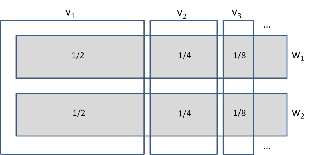
Example (Illustrated also in Figure 4). Consider a ground set with elements having unit costs. Figure 4 geometrically depicts the definition of a function , where for any set , is defined to be the area (shown shaded) covered by the elements of . Specifically, and , . Notice, . The greedy algorithm will first pick . Suppose it picks in rounds. Then . Thus, greedy will never pick or before it picks . Suppose . Clearly, the greedy solution is whereas the optimal solution is . Here can be arbitrarily large.