Scheduling with Rate Adaptation under Incomplete Knowledge of Channel/Estimator Statistics

Consider the class of stationary scheduling policies $G$ that base their decision on the current queue length information $[Q_{1},\ldots,Q_{N}]$, the channel estimates $[\widehat{C}_{i},\ldots,\widehat{C}_{N}]$, and full knowledge of channel/estimator joint statistics. Define the network stability region as the closure of the arrival rates that can be supported by the policies in $G$ without leading to system instability. Let $P_{\widehat{\bm{C}}}(\hat{\bm{c}}=[\hat{c}_{1},\ldots,\hat{c}_{N}])$ denote the probability of the channel estimate vector. Thus,

where the probabilities $P(\widehat{C}_{i}=\hat{c}_{i})$ are evaluated from the knowledge of the channel/estimator joint statistics. Defining $\mathcal{CH}[\mathcal{A}]$ as the convex hull ([16]) of set $\mathcal{A}$ and $\vec{\bm{1}}_{i}$ as the $i^{\textrm{th}}$ coordinate vector, we record our result on the network stability region below.

Proof Outline: The proof contains two parts. We first show that any rate vector $\bm{\lambda}$ strictly within $\bm{\Lambda}$ is stably supportable by some randomized stationary policy. In the second part, we establish that any arrival rate $\bm{\lambda}$ outside $\bm{\Lambda}$ is not supportable by any policy. We show this by first identifying a hyperplane that separates $\bm{\lambda}$ and $\bm{\Lambda}$ using the strict separation theorem ([17]). We then define an appropriate Lyapunov function and show that, for any scheduling policy, there exists a positive drift, thus rendering the queues unstable ([18]). Details of the proof are available in Appendix A.

In this section, we propose a maximum-weight type scheduling policy with rate adaptation and show that it is throughput-optimal, i.e., it can support any arrival rate that can be supported by any other policy in $G$. The policy is introduced next.

Scheduling Policy $\Psi$
At time slot $t$, the base station makes the scheduling and rate adaptation decisions based on the channel/estimator joint statistics and the channel estimate vector $\widehat{\bm{C}}=\hat{\bm{c}}$ (the time index is dropped for notational simplicity). (1) Rate Adaptation: For each user $i$, assign rate $R_{i}$ such that, $$R_{i}=\argmax_{r\in\mathcal{S}}\big\{P(C_{i}\geq r\big|\widehat{C}_{i}=\hat{c}_{i})\cdot r\big\}$$ (2) Scheduling Decision: Schedule the user $I$ that maximizes the queue-weighted rate $R_{i}$, as follows: $$I=\argmax_{i}\big\{Q_{i}\cdot P(C_{i}\geq R_{i}\big|\widehat{C}_{i}=\hat{c}_{i})\cdot R_{i}\big\}$$

Proof Outline: The proof proceeds as follows. Consider a Lyapunov function $L(\bm{Q}[t])=\sum_{i=1}^{N}Q_{i}^{2}[t]$. For any arrival rate $\bm{\lambda}$ that lies strictly within the stability region $\bm{\Lambda}$, we know it is stably supportable by some policy $G_{0}$. Under $G_{0}$, we show that the corresponding Lyapunov drift is negative. We then show that policy $\Psi$ minimizes the Lyapunov drift and hence it will have a negative drift, thus establishing the throughput optimality of $\Psi$.

The results obtained thus far when the channel/estimator joint statistics is available at the scheduler are along expected lines. Nonetheless, they serve as a benchmark to the rest of the work under incomplete knowledge of the channel/estimator joint statistics, which is the main focus of the paper.

With incomplete information on the channel-estimator joint statistics, the scheduler naively trusts the channel estimates to be actual channel states and transmits at the rate allowed in this state. Under this scheduling structure, for the single-hop network we consider, the stability region is given in Appendix C by

For a two-user single-hop network, this region is plotted in Fig. 1 along-side the network stability region when full knowledge of the channel/estimator joint statistics is available at the scheduler and hence rate adaptation is performed. The channel between the base station and each user is independent and binary ($\mathcal{S}=\{0.2,1\}$) with $P(C_{i}=1)=0.8,\ for\ i=1,2$. For different mismatch between the channel and the estimate, Fig. 1 plots the stability region of the system when rate adaptation is performed and when it is not. Note the significant reduction in the stability region when rate adaptation is not performed. This loss increases with increase in the degree of channel-estimator mismatch. The preceding example underscores the importance of rate adaptation and hence the need to learn the channel/estimator joint statistics. We now proceed to introduce our joint statistics learning-scheduling policy.

We design the policy with the following main components: (1) The fraction of time slots the policy spends in learning the channel/estimator joint statistics is fixed at $\gamma\in(0,1)$, (2) The worst-case rate of convergence of the statistics learning process is maximized. We formally introduce the policy next, followed by a discussion on the policy design.
Joint statistics learning-scheduling policy
(parameterized by $\gamma$)
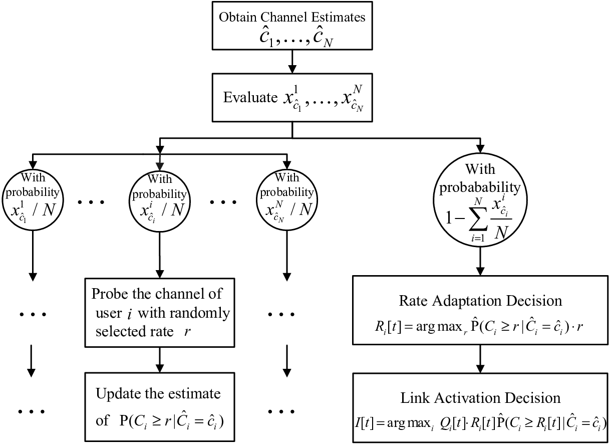
(1) In each slot, the scheduler first decides whether to explore the channel of one of the users or transmit data to one of the users. Specifically, it randomly decides to explore the channel of user $i$ with probability $x^{i}_{\hat{c}_{i}}/N$ where $\sum_{i=1}^{N}x^{i}_{\hat{c}_{i}}/N<1$. The quantity $x^{i}_{\hat{c}_{i}}\in(0,1]$ is a function of $\gamma$ and the channel estimate, $\hat{c}_{i}$, of user $i$. It is optimized to maximize the worst-case rate of convergence of the statistics learning mechanism subject to the $\gamma$ constraint. We postpone the discussion on this optimization to Proposition 4. Note that, we have dropped the time index from the estimates for ease of notation.
(2) If a user is chosen for exploration, this time slot becomes an observing slot. Call the chosen user as $e$. The scheduler now sends data at a rate $r$ that is chosen uniformly at random from the set $\mathcal{S}$. Let the quantity $\xi(t)$ indicate whether the transmission was successful or not: $\displaystyle\xi(t)=\textbf{1}(c_{e}\geq r\big),$

where, recall, $c_{e}$ denotes the current channel state of user $e$. Let $\Theta_{i,\hat{c},r}$ denote the set of exploration time slots when the channel estimate of user $i$ was $\hat{c}$ and user $i$ was explored with rate $r$. Thus, the current slot is added to the set $\Theta_{e,\hat{c}_{e},r}$. Now, an estimate of the quantity $P(C_{e}\geq r\Big|\widehat{C}_{e}=\hat{c}_{e})$ is obtained using the following update: $\displaystyle\widehat{P}_{t}(C_{e}\geq r\Big|\widehat{C}_{e}=\hat{c}_{e})=\frac{\sum_{k\in\Theta_{e,\hat{c}_{e},r}}\xi(k)}{|\Theta_{e,\hat{c}_{e},r}|}$ where $|\mathcal{V}|$ denotes the cardinality of set $\mathcal{V}$. We assume $\widehat{P}_{t}(C_{e}|\widehat{C}_{e})$ to be uniform when $\Theta_{e,\hat{c}_{e},r}=\emptyset$, i.e., $\widehat{P}_{t}(C_{e}\geq r\Big|\widehat{C}_{e}=\hat{c}_{e})=1-r/|\mathcal{S}|$. (3) With probability $1-\sum_{i=1}^{N}\frac{x^{i}_{\hat{c}_{i}}}{N}$, no user is chosen for exploration and the slot is used for data transmission. The scheduler follows policy $\Psi$ introduced in the previous section with $P(C_{i}\geq r\Big|\widehat{C}_{i}=\hat{c}_{i}\ )$ replaced by the estimate $\widehat{P}_{t}(C_{i}\geq r\Big|\widehat{C}_{i}=\hat{c}_{i}\ )$.

An illustration of the proposed policy is provided in Fig. 2. We now discuss the design of the quantities $x^{i}_{\hat{c}_{i}}$, $\hat{c}_{i}\in\mathcal{S}$, $i\in\{1,\ldots,N\}$. Let $\eta_{i,\hat{c}_{i}}=P(\widehat{C}_{i}=\hat{c}_{i})\frac{x^{i}_{\hat{c}_{i}}}{N}$ be a measure of how often the channel of user $i$ is explored when the estimate is $\hat{c}_{i}$. For fairness considerations, we impose the following constraint in addition to the $\gamma$-constraint discussed earlier:

The preceding constraint ensures that each user’s channel is explored for an equal fraction, $\gamma/N$, of the total time slots. From strong law of large numbers, with probability one, $\widehat{P}_{t}(C_{i}\geq r\Big|\widehat{C}_{i}=\hat{c}_{i})$ will converge to $P(C_{i}\geq r\Big|\widehat{C}_{i}=\hat{c}_{i})$ as $t$ tends to infinity. The rate of convergence of the channel/estimate joint statistics, parameterized by the user and the channel estimate, is given by the following lemma. Henceforth, we drop the suffix $i$ from $\hat{c}_{i}$ for notational convenience.

Note from the preceding lemma that, for each $\{i,\hat{c}\}$, the higher the quantity $\eta_{i,\hat{c}}$, the faster the convergence of $\widehat{P}_{t}(C_{i}\geq r\big|\widehat{C}_{i}=\hat{c})$. Also note that, for each user $i$, the channel estimate $\hat{c}$ with the slowest convergence affects the overall convergence performance for that user $i$. Taking note of this, we proceed to design $x^{i}_{\hat{c}}$ that maximizes the lowest convergence rate – the bottleneck.

The optimization problem $(U)$ for user $i$ is given by

For ease of exposition, we assume, without loss of generality, that $P(\widehat{C}_{i}=s_{1})\leq P(\widehat{C}_{i}=s_{2})\leq\cdots\leq P(\widehat{C}_{i}=s_{|\mathcal{S}|})$. Let $[x_{s_{1}}^{i*},x_{s_{2}}^{i*},\cdots,x_{s_{|\mathcal{S}|}}^{i*}]$ be the optimal solution to the above problem. We now record the structural properties of the optimal solution.

Proof Outline: The proof proceeds by establishing two crucial properties of the optimal solution. First, define $\Omega_{i}$ as the set of all channel estimates $s_{k}$ such that the optimal $x_{s_{k}}^{i*}=1$. Thus $\Omega_{i}=\cup_{k}\{s_{k}:\ x_{s_{k}}^{i*}=1\}$. If no such estimate exists, $\Omega_{i}=\emptyset$. The optimal solution has the following properties:

• (1)

  If $\Omega_{i}=\emptyset$ then $P(\widehat{C}_{i}=s_{k})x_{s_{k}}^{i*}=\gamma/|\mathcal{S}|,\forall k$.

• (2)

  If $\Omega_{i}\neq\emptyset$, then $x_{s_{1}}^{i*}=1$.

Recall that the channel states are ordered such that $P(\widehat{C}_{i}=s_{1})\leq P(\widehat{C}_{i}=s_{2})\leq\cdots\leq P(\widehat{C}_{i}=s_{|\mathcal{S}|})$. The first property essentially says that if there does not exist a channel estimate $s$, for which $x_{s}^{i*}=1$, then the optimal solution is such that the learning rate ($\frac{P(\widehat{C}=s_{k})x_{s_{k}}^{i*}}{N}$) is uniform ($\frac{\gamma/|\mathcal{S}|}{N}$) for all $s_{k}$, $k\in\{1,\ldots,|\mathcal{S}|\}$. Because, otherwise, there is always room to improve the bottleneck convergence rate by redesigning the quantities $x_{s_{k}}^{i*}$. The second property says that whenever there exists an estimate $s_{k,k\neq 1}$ for which $x_{s_{k}}^{i*}=1$, the estimate $s_{1}$ acts as a bottleneck, and the optimal value of $x_{s_{1}}^{i*}$ must be 1. The proposed algorithm now checks whether a solution yielding uniform convergence rate is feasible. If so, the solution is trivially given by $x_{s_{k}}^{i*}=\frac{1}{P(\widehat{C}_{i}=s_{k})}\frac{\gamma}{|\mathcal{S}|}$, for all $k\in\{1,\ldots,|\mathcal{S}|\}$. Otherwise, using the preceding properties, the algorithm assigns $x_{s_{1}}^{i*}=1$ and goes on to solve the reduced optimization problem over $x_{s_{2}}^{i*}\ldots,x_{s_{|\mathcal{S}|}}^{i*}$, iteratively. Details of the proof can be found in Appendix D.

The proposed algorithm is illustrated in Fig. 3 when $\gamma=0.2$, $N=2$ and $\mathcal{S}=\{1,\ldots,6\}$. Focusing on User $1$, Fig. 3(a) plots the probability of the estimated channels and the optimal values of $x^{1*}_{s}$, $s\in\mathcal{S}$. Note that, the lower the value of $P(\widehat{C}_{1}=s)$, the higher the assigned $x^{1*}_{s}$, since the algorithm maximizes the bottleneck convergence rate $\frac{P(\widehat{C}=s)x_{s}^{1*}}{N}$. This is further illustrated in Fig. 3(b) where the optimized convergence rate is shown to be ‘near uniform’, underlining the minmax nature of the optimization. Note that the structure of the minmax algorithm bears some similarity with the water-filling algorithm used in power allocation across parallel channels ([21]). There the algorithm tries to ‘equalize’ the sum of two components (signal and noise powers) across channels, while the minmax algorithm we propose tries to ‘equalize’ the product of two components ($P(\widehat{C}_{i}=s)$ and $x_{s}^{i*}$).

We now perform a stability region analysis of the proposed policy. Define the stability region of a policy as the exhaustive set of arrival rates such that the network queues are rendered stable under the policy. The stability region of the proposed policy, parameterized by $\gamma\in(0,1)$, is recorded below.

Proof Outline: The proof proceeds by showing that, under the proposed joint statistics learning - scheduling policy, the instantaneous maximal sum of the queue weighted achievable rates, with sufficient time, can be arbitrarily close to the case when perfect knowledge of the statistics is available. Details are provided in Appendix E.

As $\gamma\rightarrow 0$, the proposed policy has a stability region that can be arbitrarily close to the system stability region $\bm{\Lambda}$. The trade-off involved here is the speed of convergence and hence queueing delays before convergence. Since an analytical study of this trade-off appears complicated, we proceed to perform a numerical study. The simulation setup is described next.

We use i.i.d. Rayleigh fading channels with minimum mean square error (MMSE) channel estimator as seen in [22] and [23]. The channel model is given by

where $X,Y$ correspond to transmitted and received signals, $\rho$ is the average SNR at the receiver, and $\nu$ is the additive noise. Both $h$ and $\nu$ are zero-mean complex Gaussian random variables, i.e., with probability density $\mathcal{CN}(0,1)$. Let $\hat{h}$ denote the estimate of the channel and $\tilde{h}$ denote the estimation error. Under the channel statistics assumed, $\tilde{h}$ is zero-mean complex Gaussian with variance $\beta$, where the value of $\beta$ depends on the resources allocated for estimation ([24]). Given the value of $h$, the channel rate is $R=\log(1+\rho|h|^{2})$. We quantize the transmission rate to make the channel state space to be discrete and finite. We assume a two-user network and fix $\beta=0.1$ and $\rho=50$ for both users’ channels. We study the average behavior of the proposed policy by implementing it over $10000$ parallel queuing systems.

We first study the time evolution of the probability of transmission success for different values of $\gamma$. Fig. 4(a) shows that, for any $\gamma$, the probability of successful transmission increases as the accuracy of the estimate of the channel/estimator joint statistics improves with time. Also, as expected, the larger the value of $\gamma$ is, the faster is the improvement in the probability of successful transmission. Note that higher transmission success probability essentially means lesser number of retransmissions. This is illustrated in Fig. 4(b).

In Fig. 5, we study the time evolution of the average packet delay - the delay between the time a packet enters the queue and the time it leaves the head of the queue - for various values of $\gamma$. Note that $\gamma$ influences the average delay through (1) the average number of retransmissions and (2) the fraction of time slots available for transmissions. It is expected that the nature of the influence of $\gamma$ on the average delay depends on whether the estimate of the channel/estimator joint statistics has reached convergence or not. After convergence, the average delay is influenced by $\gamma$ solely through the fraction of time slots available for transmissions. Thus, after convergence, the higher the value of $\gamma$, the higher the average delay. This is illustrated in Fig. 5. Before convergence, however, the effect of $\gamma$ on the average delay is not straightforward. Fig. 5, along with the fact that higher $\gamma$ results in faster convergence, suggests the following: before convergence, $\gamma$ influences the average delay predominantly through the average number of retransmissions, resulting in decreasing average delay for increasing $\gamma$. In fact, Fig. 5 suggests the existence of a larger phenomenon: the trade-off between throughput (the stability region) and the delay before convergence.

References

• [1] L. Tassiulas, A. Ephremides, “Stability properties of constrained queueing systems and scheduling policies for maximum throughput in multihop radio networks,” IEEE Transactions on Automatic Control, vol. 37, no. 12, pp. 1936-1948, Dec. 1992.
• [2] L. Tassiulas, A. Ephremides, “Dynamic server allocation to parallel queues with randomly varying connectivity,” IEEE Transactions on Information Theory, vol. 39, no. 2, pp. 466-478, Mar. 1993.
• [3] X. Lin, N. B. Shroff. “Joint rate control and scheduling in multihop wireless networks,” Proceedings of IEEE Conference on Decision and Control, Paradise Island, Bahamas, Dec. 2004.
• [4] X. Lin, N. B. Shroff, “The impact of imperfect scheduling on cross-Layer congestion control in wireless networks,” IEEE/ACM Transaction on Networking, vol. 14, no. 2, pp. 302-315, Apr. 2006.
• [5] A. Eryilmaz, R. Srikant, “Fair resource allocation in wireless networks using queue-length based scheduling and congestion control,” IEEE/ACM Transaction on Networking, vol. 15, no. 6, pp. 1333-1344, Dec. 2007.
• [6] A. Eryilmaz, R. Srikant, “Joint congestion control, routing and MAC for stability and fairness in wireless networks,” IEEE Journal on Selected Areas in Communications, vol. 24, no. 8, pp. 1514-1524, Aug. 2006.
• [7] A. Stolyar, “Maximizing queueing network utility subject to stability: greedy primal-dual algorithm,” Queueing Systems, vol. 50, no.4, pp.401-457, Aug. 2005.
• [8] M. J. Neely, E. Modiano, C. Li, “Fairness and optimal stochastic control for heterogeneous networks,” IEEE Transactions on Information Theory, vol. 52, no. 7, pp. 2915-2934, Jul. 2006.
• [9] K. Kar, X. Luo, S. Sarkar, “Throughput-optimal scheduling in multichannel access point networks under infrequent channel measurements,” IEEE Transactions on Wireless Communications, vol. 7, no. 7, pp. 2619-2629, Jul. 2008,
• [10] L. Ying, S. Shakkottai, “Scheduling in mobile Ad Hoc networks with topology and channel-State Uncertainty,” Proceedings of IEEE INFOCOM, Rio de Janeiro, Brazil, Apr. 2009.
• [11] A. Gopalan, C. Caramanis, S. Shakkottai,“On wireless scheduling with partial channel-state information,” Proceedings of Allerton Conference on Communication, Control, and Computing, Monticello, IL, Sept. 2007.
• [12] C. Li, M. J. Neely, “Energy-optimal scheduling with dynamic channel acquisition in wireless downlinks,” Proceedings of IEEE Conference on Decision and Control, New Orleans, LA, Dec. 2007.
• [13] A. Pantelidou, A. Ephremides, A.L. Tits, “Joint scheduling and routing for Ad-hoc networks under channel state uncertainty,” Proceedings of IEEE Intl. Symp. on Modeling and Optimization in Mobile, Ad Hoc, and Wireless Networks (WiOpt), Limassol, Cyprus, Apr. 2007.
• [14] R. Aggarwal, P. Schniter, C. E. Koksal, “Rate adaptation via link-layer feedback for goodput maximization over a time-varying channel,” IEEE Transactions on Wireless Communications, vol. 8, no. 8, pp. 4276-4285, Aug. 2009.
• [15] M. J. Neely, “Max weight learning algorithms with application to scheduling in unknown environments,” arXiv:0902.0630v1, Feb. 2009.
• [16] S. Boyd, L. Vandenberghe, “Convex optimization,” Cambridge University Press, 2004.
• [17] D. Bertsekas, “Nonlinear Programming,” Belmont, MA: Athena Scientific, 1995.
• [18] S. Meyn, “Control techniques for complex networks,” Cambridge University Press, 2007.
• [19] P. Billingsley, “Probability and measure, 3rd edition,” Wiley, New York, 1995.
• [20] R. G. Gallager, “Discrete stochastic processes,” Boston, MA: Kluwer, 1996.
• [21] D. Tse, P. Viswanath, “Fundamentals of wireless communication,” Cambridge University Press, 2005.
• [22] D. Zheng, S. Pun, W. Ge, J. Zhang, H.V. Poor, “Distributed opportunistic scheduling for Ad-Hoc communications under noisy channel estimation,” Proceedings of IEEE ICC, Beijing, China May 2008.
• [23] A. Vakili, M. Sharif, B. Hassibi, “The effect of channel estimation error on the throughput of broadcast channels,” Proceedings of IEEE Int. Conf. Acoust. Speech Signal Processing, Toulouse, France, May 2006.
• [24] T. Kailath, A.H. Sayed, B. Hassibi, “Linear estimation,” Prentice-Hall, 2000.
Appendix A Proof of Proposition 1
Proof.
(Sufficiency) Define the Lyapunov function L⁡(𝑸⁡[t])=∑i=1NQi2​[t]L(\bm{Q}[t])=\sum_{i=1}^{N}Q^{2}_{i}[t]. Recall the queue dynamic equation given by Equation (1), the Lyapunov drift can be written as
Δ​L​[t]\displaystyle\Delta L[t] =E⁡[∑i=1NQi2​[t+1]−Qi2​[t]|𝑸⁡[t]]\displaystyle=E\Big[\sum_{i=1}^{N}Q_{i}^{2}[t+1]-Q_{i}^{2}[t]\Big|\ \bm{Q}[t]\ \Big]
≤B+2​∑i=1NQi​[t]​(λi−E⁡[𝟏​(I⁡[t]=i)⋅R⁡[t]⋅𝟏​(R⁡[t]≤Ci​[t])|𝑸⁡[t]])\displaystyle\leq B+2\sum_{i=1}^{N}Q_{i}[t]\Big(\lambda_{i}-\ E\Big[\bm{1}(I[t]=i)\cdot R[t]\cdot\bm{1}(R[t]\leq C_{i}[t])\Big|\ \bm{Q}[t]\ \Big]\ \Big) (7)
where
B=∑i=1NE⁡[𝟏​(I⁡[t]=i)⋅R2​[t]​𝟏​(R⁡[t]≤Ci​[t])+Ai2​[t]|𝑸⁡[t]].\displaystyle B=\sum_{i=1}^{N}E\big[\bm{1}(I[t]=i)\cdot R^{2}[t]\bm{1}(R[t]\leq C_{i}[t])+A_{i}^{2}[t]\Big|\ \bm{Q}[t]\big].
Noting that BB is bounded. Let ri∗​(c^i)=arg⁡maxri⁡P⁡(Ci≥ri|C^i=c^i)⋅rir_{i}^{*}(\hat{c}_{i})=\arg\max_{r_{i}}P(C_{i}\geq r_{i}\big|\widehat{C}_{i}=\hat{c}_{i}\ )\cdot r_{i}. Consider any arrival vector 𝝀\bm{\lambda} strictly within the interior of 𝚲\bm{\Lambda}. For each channel state 𝒄^\hat{\bm{c}}, there exist scaling vector 𝜶𝒄^\bm{\alpha}^{\hat{\bm{c}}} and δ>0\delta>0 associated with it such that
λi+δ<∑𝒄^∈𝒮Nπ^𝒄^⋅αi𝒄^⋅P⁡(Ci≥ri∗​(c^i)|C^i=c^i)⋅ri∗​(c^i),\displaystyle\lambda_{i}+\delta<\sum_{\hat{\bm{c}}\in\mathcal{S}^{N}}\hat{\pi}_{\hat{\bm{c}}}\cdot\alpha_{i}^{\hat{\bm{c}}}\cdot P(C_{i}\geq r_{i}^{*}(\hat{c}_{i})\big|\widehat{C}_{i}=\hat{c}_{i}\ )\cdot r_{i}^{*}(\hat{c}_{i}), (8)
for any user ii, where ∑i=1Nαi𝒄^=1\sum_{i=1}^{N}\alpha_{i}^{\hat{\bm{c}}}=1 for ∀𝒄^\forall\hat{\bm{c}}.
Therefore, we can design a scheduling policy that does the following: At the channel estimation 𝑪^​[t]=𝒄^​[t]\widehat{\bm{C}}[t]=\hat{\bm{c}}[t], channel ii is activated with probability αi𝒄^\alpha_{i}^{\hat{\bm{c}}}. The rate allocated to channel ii will be ri∗​(c^i​[t])r_{i}^{*}(\hat{c}_{i}[t]).
Then the service rate of user ii will be:
μi=E⁡[𝟏​(I⁡[t]=i)⋅Ri​[t]⋅𝟏​(Ri​[t]≤Ci​[t])]=∑𝒄^∈𝒮Nπ𝒄^⋅αi𝒄^⋅P⁡(Ci≥ri∗​(c^i)|C^i=c^i)⋅ri∗​(c^i)\displaystyle\mu_{i}=E\big[\bm{1}(I[t]=i)\cdot R_{i}[t]\cdot\bm{1}(R_{i}[t]\leq C_{i}[t])\big]=\sum_{\hat{\bm{c}}\in\mathcal{S}^{N}}\pi_{\hat{\bm{c}}}\cdot\alpha_{i}^{\hat{\bm{c}}}\cdot P(C_{i}\geq r_{i}^{*}(\hat{c}_{i})\big|\widehat{C}_{i}=\hat{c}_{i}\ )\cdot r_{i}^{*}(\hat{c}_{i}) (9)
Substitute (9) to (8) we have
λi−μi<−δ.\displaystyle\lambda_{i}-\mu_{i}<-\delta. (10)
Noting that in this policy the rate adaptation and link activation is completely determined by the channel estimation, and does not rely on queue length information, and therefore in this case
OPENOPENE⁡[𝟏​(I⁡[t]=i)⋅R⁡[t]⋅𝟏​(R⁡[t]≤Ci​[t])|𝑸⁡[t]])=E⁡[𝟏​(I⁡[t]=i)⋅R⁡[t]⋅𝟏​(R⁡[t]≤Ci​[t])])=μi\displaystyle E\Big[\bm{1}(I[t]=i)\cdot R[t]\cdot\bm{1}(R[t]\leq C_{i}[t])\Big|\ \bm{Q}[t]\ \Big]\ \Big)=E\Big[\bm{1}(I[t]=i)\cdot R[t]\cdot\bm{1}(R[t]\leq C_{i}[t])\ \Big]\ \Big)=\mu_{i} (11)
Substitute (10) (11) into (7), the Lyapunov drift function now becomes
Δ​L​[t]≤B−2​δ​∑i=1NQi​[t].\displaystyle\Delta L[t]\leq B-2\delta\sum_{i=1}^{N}Q_{i}[t].
Because the scheduling and rate adaptation decision only depends on the current queue length and current channel estimate state, the queue evolves as a Markov Chain. According to Foster-Lyapunov Stability criterion [18], the queues will be stable.
(Necessity) From strict separation theorem [17], for any arrival rate vector out side the proposed region 𝚲\bm{\Lambda}, there exist 𝜷\bm{\beta}, δ>0\delta>0, such that for any vector 𝝂→\vec{\bm{\nu}} inside the stability region 𝚲\bm{\Lambda}
∑i=1Nβi​(λi−νi)≥δ\displaystyle\sum_{i=1}^{N}\beta_{i}(\lambda_{i}-\nu_{i})\geq\delta
Define Lyapunov function L⁡(𝑸⁡[t])=∑i=1Nβi​Qi​[t]L(\bm{Q}[t])=\sum_{i=1}^{N}\beta_{i}Q_{i}[t]. For any stationary scheduling policy that makes I⁡[t]I[t] and R⁡[t]R[t] decisions, we will have the following Lyapunov drift expression
E⁡[L⁡(𝑸⁡[t+1])−L⁡(𝑸⁡[t])|𝑸⁡[t]]=\displaystyle E\Big[L(\bm{Q}[t+1])-L(\bm{Q}[t])\Big|\bm{Q}[t]\Big]= ∑i=1Nβi​E​[Ai​[t]−𝟏​(I⁡[t]=i)⋅𝟏​(Ri​[t]≤Ci​[t])⋅Ri​[t]|𝑸⁡[t]]\displaystyle\sum_{i=1}^{N}\beta_{i}E\Big[A_{i}[t]-\bm{1}(I[t]=i)\cdot\bm{1}(R_{i}[t]\leq C_{i}[t])\cdot R_{i}[t]\Big|\bm{Q}[t]\Big]
=\displaystyle= ∑i=1Nβi​[λi−E⁡[𝟏​(I⁡[t]=i)⋅𝟏​(Ri​[t]≤Ci​[t])⋅Ri​[t]|𝑸⁡[t]]]\displaystyle\sum_{i=1}^{N}\beta_{i}\Big[\lambda_{i}-E\big[\bm{1}(I[t]=i)\cdot\bm{1}(R_{i}[t]\leq C_{i}[t])\cdot R_{i}[t]\Big|\bm{Q}[t]\big]\Big] (12)
Let μi=E[𝟏(I[t]=i)⋅𝟏(Ri[t]≤Ci[t])⋅Ri[t]|𝑸[t]]]\mu_{i}=E\big[\bm{1}(I[t]=i)\cdot\bm{1}(R_{i}[t]\leq C_{i}[t])\cdot R_{i}[t]\Big|\bm{Q}[t]\big]\Big].
Next we are going to show that 𝝁→∈𝚲\vec{\bm{\mu}}\in\bm{\Lambda}. Consider
E[𝟏(I[t]=i)⋅𝟏(Ri[t]≤Ci[t])⋅Ri[t]|𝑸[t]]]\displaystyle E\Big[\bm{1}(I[t]=i)\cdot\bm{1}(R_{i}[t]\leq C_{i}[t])\cdot R_{i}[t]\Big|\bm{Q}[t]\big]\Big]
=\displaystyle= E[E[𝟏(I[t]=i)⋅𝟏(Ri[t]≤Ci[t])⋅Ri[t]|𝑸[t];𝑪^[t]]]\displaystyle E\Big[E\big[\bm{1}(I[t]=i)\cdot\bm{1}(R_{i}[t]\leq C_{i}[t])\cdot R_{i}[t]\Big|\bm{Q}[t];\widehat{\bm{C}}[t]\big]\Big]
=\displaystyle= ∑𝒄t^∈𝒮Nπ𝒄^t⋅E[𝟏(I[t]=i)⋅𝟏(Ri[t]≤Ci[t])⋅Ri[t]|𝑸[t];𝑪^[t]=𝒄^t]\displaystyle\mathop{\sum}_{\hat{\bm{c}_{t}}\in\mathcal{S}^{N}}\pi_{\hat{\bm{c}}_{t}}\cdot E\Big[\bm{1}(I[t]=i)\cdot\bm{1}(R_{i}[t]\leq C_{i}[t])\cdot R_{i}[t]\Big|\bm{Q}[t];\widehat{\bm{C}}[t]=\hat{\bm{c}}_{t}\Big]
=\displaystyle= ∑𝒄^∈𝒮Nπ𝒄^⋅𝟏​(I⁡[t]=i)⋅Ri​[t]⋅P​r​(Ri​[t]≤Ci​[t]|C^i​[t]=c^)\displaystyle\sum_{\hat{\bm{c}}\in\mathcal{S}^{N}}\pi_{\hat{\bm{c}}}\cdot\bm{1}(I[t]=i)\cdot R_{i}[t]\cdot Pr\big(R_{i}[t]\leq C_{i}[t]\Big|\widehat{C}_{i}[t]=\hat{c}\big)
≤\displaystyle\leq ∑𝒄^∈𝒮Nπ𝒄^⋅𝟏​(I⁡[t]=i)⋅ri∗​(c^i​[t])⋅P​r​(ri∗​(c^i​[t])≤Ci​[t]|C^i​[t]=c^i​[t]).\displaystyle\sum_{\hat{\bm{c}}\in\mathcal{S}^{N}}\pi_{\hat{\bm{c}}}\cdot\bm{1}(I[t]=i)\cdot r_{i}^{*}(\hat{c}_{i}[t])\cdot Pr\big(r_{i}^{*}(\hat{c}_{i}[t])\leq C_{i}[t]\Big|\widehat{C}_{i}[t]=\hat{c}_{i}[t]\big).
The third equality holds because R⁡[t]R[t] and I⁡[t]I[t] is determined by the current channel estimation and queue length information within the class G of stationary policies, and also the i.i.d. channel assumption. The above expression indicates that 𝝁→∈𝚲\vec{\bm{\mu}}\in\bm{\Lambda}. Hence from (12)
E⁡[L⁡(𝑸⁡[t+1])−L⁡(𝑸⁡[t])|𝑸⁡[t]]\displaystyle E\Big[L(\bm{Q}[t+1])-L(\bm{Q}[t])\Big|\bm{Q}[t]\Big] =∑i=1Nβi​[λi−E⁡[𝟏​(I⁡[t]=i)⋅𝟏​(Ri​[t]≤Ci​[t])⋅Ri​[t]|𝑸⁡[t]]]\displaystyle=\sum_{i=1}^{N}\beta_{i}\Big[\lambda_{i}-E\big[\bm{1}(I[t]=i)\cdot\bm{1}(R_{i}[t]\leq C_{i}[t])\cdot R_{i}[t]\Big|\bm{Q}[t]\big]\Big]
≥δ\displaystyle\geq\delta
The Lyapunov function will always have a positive drift and therefore, the queue is unstable. ∎
Appendix B Proof of Proposition 2
Assume the arrival rate vector 𝝀\bm{\lambda} is strictly within the interior of stability region, there exists ε>0\varepsilon>0 such that 𝝀+ε​𝟏→∈i​n​t​(𝚲)\bm{\lambda}+\varepsilon\vec{\bm{1}}\in int(\bm{\Lambda}). Because 𝝀\bm{\lambda} is strictly within the stability region, similar to the proof of Proposition 1, there exists some randomized scheduling policy G0G_{0} that stably supports the arrival rate vector 𝝀+ε​𝟏→\bm{\lambda}+\varepsilon\vec{\bm{1}}, and that G0G_{0} will only depends on the estimated channel state.
Suppose the proposed scheduling policy Ψ\Psi will result in rate allocation Ri​[t]R_{i}[t] and scheduling decision I⁡[t]I[t] at time tt. Consider the policy G0G_{0} that act at the same time tt with the same channel state estimate and queue lengths knowledge, we denote its rate allocation to be R~i​[t]\widetilde{R}_{i}[t] and link activation decision to be I~​[t]\widetilde{I}[t], therefore we have
∑i=1NQi​[t]⋅E⁡[𝟏​(I~​[t]=i)⋅R~​[t]⋅𝟏​(R~​[t]≤Ci​[t])]\displaystyle\sum_{i=1}^{N}Q_{i}[t]\cdot E\Big[\bm{1}(\widetilde{I}[t]=i)\cdot\widetilde{R}[t]\cdot\bm{1}(\widetilde{R}[t]\leq C_{i}[t])\ \Big]
=\displaystyle= ∑i=1NQi[t]⋅E[E[𝟏(I~[t]=i)⋅R~[t]⋅𝟏(R~[t]≤Ci[t])|𝑸[t],𝑪^[t]]]\displaystyle\sum_{i=1}^{N}Q_{i}[t]\cdot E\Big[E\Big[\bm{1}(\widetilde{I}[t]=i)\cdot\widetilde{R}[t]\cdot\bm{1}(\widetilde{R}[t]\leq C_{i}[t])\Big|\ \bm{Q}[t],\ \widehat{\bm{C}}[t]\Big]\ \Big]
≤\displaystyle\leq ∑i=1NQi[t]⋅E[E[𝟏(I[t]=i)⋅R[t]⋅𝟏(R[t]≤Ci[t])|𝑸[t],𝑪^[t]]].\displaystyle\sum_{i=1}^{N}Q_{i}[t]\cdot E\Big[E\Big[\bm{1}(I[t]=i)\cdot R[t]\cdot\bm{1}(R[t]\leq C_{i}[t])\Big|\ \bm{Q}[t],\ \widehat{\bm{C}}[t]\Big]\ \Big].
The last inequality holds because policy Ψ\Psi maximizes the left hand side of the above inequality at every time slot. Also because the queue of each user is stable under policy G0G_{0}, we have
λi+ε\displaystyle\lambda_{i}+\varepsilon ≤E⁡[𝟏​(I~​[t]=i)⋅R~i​[t]⋅𝟏​(R~i​[t]≤Ci​[t])]\displaystyle\leq E\Big[\bm{1}(\widetilde{I}[t]=i)\cdot\widetilde{R}_{i}[t]\cdot\bm{1}(\widetilde{R}_{i}[t]\leq C_{i}[t])\Big]
And therefore
∑i=1NQi​[t]⋅(λi+ε)\displaystyle\sum_{i=1}^{N}Q_{i}[t]\cdot(\lambda_{i}+\varepsilon) ≤∑i=1NQi​[t]⋅E⁡[𝟏​(I~​[t]=i)⋅R~i​[t]⋅𝟏​(R~i​[t]≤Ci​[t])]\displaystyle\leq\sum_{i=1}^{N}Q_{i}[t]\cdot E\Big[\bm{1}(\widetilde{I}[t]=i)\cdot\widetilde{R}_{i}[t]\cdot\bm{1}(\widetilde{R}_{i}[t]\leq C_{i}[t])\Big]
≤∑i=1NQi[t]⋅E[E[𝟏(I[t]=i)⋅R[t]⋅𝟏(R[t]≤Ci[t])|𝑸[t],𝑪^[t]]]\displaystyle\leq\sum_{i=1}^{N}Q_{i}[t]\cdot E\Big[E\Big[\bm{1}(I[t]=i)\cdot R[t]\cdot\bm{1}(R[t]\leq C_{i}[t])\Big|\ \bm{Q}[t],\ \widehat{\bm{C}}[t]\Big]\ \Big]
Substitute it back to Lyapunov drift expression (7), then we will have:
Δ​L​[t]\displaystyle\Delta L[t] ≤B+2∑i=1NQi[t](λi−E[E[𝟏(I[t]=i)⋅R[t]⋅𝟏(R[t]≤Ci[t])|𝑸[t],𝑪^[t]]])\displaystyle\leq B+2\sum_{i=1}^{N}Q_{i}[t]\Big(\lambda_{i}-E\Big[E\Big[\bm{1}(I[t]=i)\cdot R[t]\cdot\bm{1}(R[t]\leq C_{i}[t])\Big|\ \bm{Q}[t],\ \widehat{\bm{C}}[t]\Big]\ \Big]\Big)
≤B−2​ε​∑i=1NQi​[t]\displaystyle\leq B-2\varepsilon\sum_{i=1}^{N}Q_{i}[t]
Because scheduling policy Ψ\Psi only depends on current queue length and channel estimate, and because the channel process is a i.i.d. across time, the queue evolution under policy Ψ\Psi will be a Markov Chain. From Foster-Lyapunov criterion, the statement is proven. ∎
Appendix C Proof of Stability Region Without Rate Adaptation
The proof of the statement is somehow similar to proof of proposition 1.
(Sufficiency) Define the Lyapunov function L⁡(𝑸⁡[t])=∑i=1NQi2​[t]L(\bm{Q}[t])=\sum_{i=1}^{N}Q^{2}_{i}[t], the Lyapunov drift can be written as Equation (7). For any arrival vector 𝝀\bm{\lambda} strictly within the interior of 𝚲~\tilde{\bm{\Lambda}} and each channel state 𝒄^\hat{\bm{c}}, the vector 𝜶𝒄^\bm{\alpha}^{\hat{\bm{c}}} and δ>0\delta>0 satisfies
λi+δ<∑𝒄^∈𝒮Nπ^𝒄^⋅αi𝒄^⋅P⁡(Ci≥c^i|C^i=c^i)⋅c^i,\displaystyle\lambda_{i}+\delta<\sum_{\hat{\bm{c}}\in\mathcal{S}^{N}}\hat{\pi}_{\hat{\bm{c}}}\cdot\alpha_{i}^{\hat{\bm{c}}}\cdot P(C_{i}\geq\hat{c}_{i}\big|\widehat{C}_{i}=\hat{c}_{i}\ )\cdot\hat{c}_{i},
The rest of the proof follows similar as in Proposition 1.
(Necessity) Similar to the proof of Proposition 1, for any arrival rate vector out side 𝚲~\tilde{\bm{\Lambda}}, there exist 𝜷\bm{\beta}, δ>0\delta>0, such that for any vector 𝝂→\vec{\bm{\nu}} inside the stability region 𝚲~\tilde{\bm{\Lambda}}, we have ∑i=1Nβi​(λi−νi)≥δ\sum_{i=1}^{N}\beta_{i}(\lambda_{i}-\nu_{i})\geq\delta.
Define Lyapunov function L⁡(𝑸⁡[t])=∑i=1Nβi​Qi​[t]L(\bm{Q}[t])=\sum_{i=1}^{N}\beta_{i}Q_{i}[t], for any stationary policy that makes scheduling decision I⁡[t]I[t] and rate adaptation decision R⁡[t]R[t], again we will have the similar Lyapunov drift expression as in Equation (12),
E⁡[L⁡(𝑸⁡[t+1])−L⁡(𝑸⁡[t])|𝑸⁡[t]]=∑i=1Nβi⋅[λi−E⁡[𝟏​(I⁡[t]=i)⋅𝟏​(C^i​[t]≤Ci​[t])⋅C^i​[t]|𝑸⁡[t]]]\displaystyle E\Big[L(\bm{Q}[t+1])-L(\bm{Q}[t])\Big|\bm{Q}[t]\Big]=\sum_{i=1}^{N}\beta_{i}\cdot\Big[\lambda_{i}-E\big[\bm{1}(I[t]=i)\cdot\bm{1}(\widehat{C}_{i}[t]\leq C_{i}[t])\cdot\widehat{C}_{i}[t]\Big|\bm{Q}[t]\big]\Big]
Let μi=E[𝟏(I[t]=i)⋅𝟏(C^i[t]≤Ci[t])⋅C^i[t]|𝑸[t]]]\mu_{i}=E\big[\bm{1}(I[t]=i)\cdot\bm{1}(\widehat{C}_{i}[t]\leq C_{i}[t])\cdot\widehat{C}_{i}[t]\Big|\bm{Q}[t]\big]\Big]. We can show 𝝁→∈𝚲~\vec{\bm{\mu}}\in\tilde{\bm{\Lambda}} from
E[𝟏(I[t]=i)⋅𝟏(C^i[t]≤Ci[t])⋅C^i|𝑸[t]]]=\displaystyle E\Big[\bm{1}(I[t]=i)\cdot\bm{1}(\widehat{C}_{i}[t]\leq C_{i}[t])\cdot\widehat{C}_{i}\Big|\bm{Q}[t]\big]\Big]= E[E[𝟏(I[t]=i)⋅𝟏(C^i[t]≤Ci[t])⋅C^i[t]|𝑸[t];𝑪^[t]]]\displaystyle E\Big[E\big[\bm{1}(I[t]=i)\cdot\bm{1}(\widehat{C}_{i}[t]\leq C_{i}[t])\cdot\widehat{C}_{i}[t]\Big|\bm{Q}[t];\widehat{\bm{C}}[t]\big]\Big]
=\displaystyle= ∑𝒄^∈𝒮Nπ𝒄^⋅𝟏​(I⁡[t]=i)⋅c^i⋅P​r​(c^i≤Ci​[t]|C^i​[t]=c^i)\displaystyle\sum_{\hat{\bm{c}}\in\mathcal{S}^{N}}\pi_{\hat{\bm{c}}}\cdot\bm{1}(I[t]=i)\cdot\hat{c}_{i}\cdot Pr\big(\hat{c}_{i}\leq C_{i}[t]\Big|\widehat{C}_{i}[t]=\hat{c}_{i}\big)
=\displaystyle= ∑𝒄^∈𝒮Nπ𝒄^⋅𝟏​(I⁡[t]=i)⋅c^i⋅P​r​(c^i≤Ci​[t]|C^i​[t]=c^i).\displaystyle\sum_{\hat{\bm{c}}\in\mathcal{S}^{N}}\pi_{\hat{\bm{c}}}\cdot\bm{1}(I[t]=i)\cdot\hat{c}_{i}\cdot Pr\big(\hat{c}_{i}\leq C_{i}[t]\Big|\widehat{C}_{i}[t]=\hat{c}_{i}\big).
The rest follows similarly as in proof of Proposition 1. ∎
Appendix D Proof of Proposition 4
For notational convenience, we drop user index ii in the proof. The optimization problem (U) can be re-written as
maxxc^minc^\displaystyle\max_{x_{\hat{c}}}\quad\min_{\hat{c}}\quad P​r​(C^=c^)​xc^\displaystyle Pr(\widehat{C}=\hat{c})x_{\hat{c}}
s.t.\displaystyle\ s.t.\hskip 9.97537pt\qquad ∑c^∈𝒮P​r​(C^=c^)​xc^=γ\displaystyle\sum_{\hat{c}\in\mathcal{S}}Pr(\widehat{C}=\hat{c})x_{\hat{c}}=\gamma
∑c^∈𝒮P​r​(C^=c^)=1\displaystyle\sum_{\hat{c}\in\mathcal{S}}Pr(\widehat{C}=\hat{c})=1
0<xc^≤1.\displaystyle 0<x_{\hat{c}}\leq 1.
This problem can be transformed into a Linear Programming problem as the following.
max\displaystyle\max\quad t\displaystyle t
s.t.\displaystyle s.t.\quad Pr⁡(C^=c^)​xc^≥t\displaystyle\Pr(\widehat{C}=\hat{c})x_{\hat{c}}\geq t
∑c^∈𝒮P​r​(C^=c^)​xc^=γ\displaystyle\sum_{\hat{c}\in\mathcal{S}}Pr(\widehat{C}=\hat{c})x_{\hat{c}}=\gamma
Hence the problem has become a convex optimization problem. We let [t∗,xs1∗,xs2∗,⋯,xs|𝒮|∗][t^{*},x_{s_{1}}^{*},x_{s_{2}}^{*},\cdots,x_{s_{|\mathcal{S}|}}^{*}] be the optimal solution to the above problem and let Ω={sk:xsk∗=1}\Omega=\{s_{k}:\ x_{s_{k}}^{*}=1\}.
Lemma 6.
The optimal solution to the optimization problem (U) must satisfy the following structural properties:
(i) If Ω=∅\Omega=\emptyset then P​r​(C^=sk)​xsk∗=γ/|𝒮|Pr(\widehat{C}=s_{k})x_{s_{k}}^{*}=\gamma/|\mathcal{S}| for all kk.
(ii) Conversely, if P​r​(C^=sk)​xsk∗=γ|𝒮|Pr(\widehat{C}=s_{k})x_{s_{k}}^{*}=\frac{\gamma}{|\mathcal{S}|} for all kk, then Ω=∅\Omega=\emptyset, except for when P​r​(C^=s1)=γ|𝒮|Pr(\widehat{C}=s_{1})=\frac{\gamma}{|\mathcal{S}|}.
(i). Suppose Ω=∅\Omega=\emptyset but we don’t have P​r​(C^=sk)​xsk∗=γsPr(\widehat{C}=s_{k})x_{s_{k}}^{*}=\frac{\gamma}{s} for all kk. Let nn be such that t∗=P​r​(C^=sn)​xsn∗t^{*}=Pr(\widehat{C}=s_{n})x_{s_{n}}^{*}. Because P​r​(C^=sk)​xsk∗Pr(\widehat{C}=s_{k})x_{s_{k}}^{*} values are not equal for every kk, there exists m≠nm\neq n such that t∗=P​r​(C^=sn)​xsn∗<P​r​(C^=sm)​xsm∗t^{*}=Pr(\widehat{C}=s_{n})x_{s_{n}}^{*}<Pr(\widehat{C}=s_{m})x_{s_{m}}^{*}.
Because Ω=∅\Omega=\emptyset, xsn∗≠1x_{s_{n}}^{*}\neq 1 and xsm∗≠1x_{s_{m}}^{*}\neq 1. Let Π={xsk∗:t∗=P​r​(C^=sk)​xsk∗}\Pi=\{x_{s_{k}}^{*}:t^{*}=Pr(\widehat{C}=s_{k})x_{s_{k}}^{*}\} and let |Π|=π|\Pi|=\pi. If we set
xsl+\displaystyle x_{s_{l}}^{+} =xsl∗+δπ​P​r​(C^=sl),∀l∈Π\displaystyle=x_{s_{l}}^{*}+\frac{\delta}{\pi Pr(\widehat{C}=s_{l})},\ \forall l\in\Pi
xsm−\displaystyle x_{s_{m}}^{-} =xsm∗−δP​r​(C^=sm)\displaystyle=x_{s_{m}}^{*}-\frac{\delta}{Pr(\widehat{C}=s_{m})}
where δ>0\delta>0 is small that will guarantee that xsm−x_{s_{m}}^{-} stays positive.
We can check that in this case, still ∑c^i≠mc^i∉ΠP​r​(C^=ci^)​xsk∗+∑c^l∈ΠP​r​(C^=cl^)​xsl++P​r​(C^=cm^)​xsm−=γ\mathop{\sum}_{\hat{c}_{i}\neq m\atop\hat{c}_{i}\not\in\Pi}Pr(\widehat{C}{=}\hat{c_{i}})x_{s_{k}}^{*}{+}\sum_{\hat{c}_{l}\in\Pi}Pr(\widehat{C}{=}\hat{c_{l}})x_{s_{l}}^{+}{+}Pr(\widehat{C}=\hat{c_{m}})x_{s_{m}}^{-}{=}\gamma.
But in this case the new value of the objective function tn​e​w∗>t∗t_{new}^{*}>t^{*}, contradicts to the assumption that t∗t^{*} is the optimal value. Therefore we must have P​r​(C^=sk)​xsk∗=γ|𝒮|,∀iPr(\widehat{C}=s_{k})x_{s_{k}}^{*}=\frac{\gamma}{|\mathcal{S}|},\forall i, establishing the proof of (i).
(ii). When P​r​(C^=sk)​xsk∗=γ|𝒮|,∀kPr(\widehat{C}=s_{k})x_{s_{k}}^{*}=\frac{\gamma}{|\mathcal{S}|},\forall k, and xsk∗<1x_{s_{k}}^{*}<1 for all kk, we will have Ω=∅\Omega=\emptyset.
If ∃h,P​r​(C^=sh)=γ/|𝒮|\exists h,Pr(\widehat{C}=s_{h})=\gamma/|\mathcal{S}|, hence xsh∗=1x_{s_{h}}^{*}=1. By assumption
P​r​(C^=s1)​xs1∗=P​r​(C^=sh)​xsh∗=P​r​(C^=sh).\displaystyle Pr(\widehat{C}=s_{1})x_{s_{1}}^{*}=Pr(\widehat{C}=s_{h})x_{s_{h}}^{*}=Pr(\widehat{C}=s_{h}).
Because P​r​(C^=s1)≤P​r​(C^=sh)Pr(\widehat{C}=s_{1})\leq Pr(\widehat{C}=s_{h}) and xs1∗≤1x_{s_{1}}^{*}\leq 1, we must have P​r​(C^=s1)=P​r​(C^=sh)Pr(\widehat{C}=s_{1})=Pr(\widehat{C}=s_{h}) and xs1∗=1x_{s_{1}}^{*}=1, establishing the proof of (ii). ∎
Lemma 7.
If Ω≠∅\Omega\neq\emptyset, then xs1∗=1x_{s_{1}}^{*}=1 and t∗=P​r​(C^=s1)t^{*}=Pr(\widehat{C}=s_{1}).
We proof this Lemma by contradiction. Suppose that xs1∗<1x_{s_{1}}^{*}<1.
(Case 1). If t∗=P​r​(C^=s1)​xs1∗t^{*}=Pr(\widehat{C}=s_{1})x_{s_{1}}^{*}, without loss of generality, suppose s1s_{1} is the only channel state that results in P​r​(C^=s1)​xs1∗=t∗Pr(\widehat{C}=s_{1})x_{s_{1}}^{*}=t^{*}. Because Ω≠∅\Omega\neq\emptyset, suppose xsj∗=1x_{s_{j}}^{*}=1 for some state sjs_{j}. If we set xsjn​e​w=1−δ/P​r​(C^=sj)x_{s_{j}}^{new}=1-\delta/Pr(\widehat{C}=s_{j}) and xs1n​e​w=xs1∗+δ/P​r​(C^=s1)x_{s_{1}}^{new}=x_{s_{1}}^{*}+\delta/Pr(\widehat{C}=s_{1}), where δ\delta is small enough, we will get an new value of the objective function strictly larger than t∗t^{*} while still satisfy the constraints in (U), which contradicts to the optimality of [t∗,xs1∗,xs2∗,⋯,xs𝒮∗][t^{*},x_{s_{1}}^{*},x_{s_{2}}^{*},\cdots,x_{s_{\mathcal{S}}}^{*}].
(Case 2). If t∗<P​r​(C^=s1)​xs1∗t^{*}<Pr(\widehat{C}=s_{1})x_{s_{1}}^{*}, suppose t∗=P​r​(C^=sm)​xsm∗t^{*}=Pr(\widehat{C}=s_{m})x_{s_{m}}^{*} for some sms_{m} and assume, with no loss of generality, it is the only state of this kind. Because P​r​(C^=sm)​xsm∗<P​r​(C^=s1)​xs1∗Pr(\widehat{C}=s_{m})x_{s_{m}}^{*}<Pr(\widehat{C}=s_{1})x_{s_{1}}^{*} and P​r​(C^=sm)≥P​r​(C^=s1)Pr(\widehat{C}=s_{m})\geq Pr(\widehat{C}=s_{1}), we have xsm∗<xs1∗<1x_{s_{m}}^{*}<x_{s_{1}}^{*}<1. We can set xsmn​e​w=xsm∗+δ/P​r​(C^=sm)x_{s_{m}}^{new}=x_{s_{m}}^{*}+\delta/Pr(\widehat{C}=s_{m}) and xs1n​e​w=xs1∗−δ/P​r​(C^=s1)x_{s_{1}}^{new}=x_{s_{1}}^{*}-\delta/Pr(\widehat{C}=s_{1}) for δ\delta small. Again, this change of variables will result in an new objective function value strictly larger than t∗t^{*}, contradicts to the optimality of t∗t^{*}.
Therefore, we have xs1∗=1x_{s_{1}}^{*}=1.
Suppose we have t∗<P​r​(C^=s1)​xs1∗t^{*}<Pr(\widehat{C}=s_{1})x_{s_{1}}^{*}. Similar to case 2, suppose t∗=P​r​(C^=sm)​xsm∗t^{*}=Pr(\widehat{C}=s_{m})x_{s_{m}}^{*} for some sms_{m}, and assume such sms_{m} is unique, we will have xsm∗<1x_{s_{m}}^{*}<1 because P​r​(C^=sm)≥P​r​(C^=s1)Pr(\widehat{C}=s_{m})\geq Pr(\widehat{C}=s_{1}). By letting xsmn​e​w=1+δ/P​r​(C^=sm)x_{s_{m}}^{new}=1+\delta/Pr(\widehat{C}=s_{m}) and xs1n​e​w=1−δ/P​r​(C^=s1)x_{s_{1}}^{new}=1-\delta/Pr(\widehat{C}=s_{1}) with δ\delta small, we can get a strictly larger objective function value, contradicting to the optimality of t∗t^{*}. Therefore we must have t∗=P​r​(C^=s1)​xs1∗t^{*}=Pr(\widehat{C}=s_{1})x_{s_{1}}^{*}. ∎
After we have established the above lemmas, we proceed to the proof of Proposition 4.
(Proof of Proposition 4)
(Case 1). First consider the case when P​r​(C^=s1)>γ|𝒮|Pr(\widehat{C}=s_{1})>\frac{\gamma}{|\mathcal{S}|}. If in this case Ω≠∅\Omega\neq\emptyset, then from Lemma 7, t∗=P​r​(C^=s1)>γ|𝒮|t^{*}=Pr(\widehat{C}=s_{1})>\frac{\gamma}{|\mathcal{S}|}. Then ∑k=1|𝒮|P​r​(C^=sk)​xsk∗≥|𝒮|⋅t∗>|𝒮|⋅γ|𝒮|=γ\sum_{k=1}^{|\mathcal{S}|}Pr(\widehat{C}=s_{k})x_{s_{k}}^{*}\geq|\mathcal{S}|\cdot t^{*}>|\mathcal{S}|\cdot\frac{\gamma}{|\mathcal{S}|}=\gamma. Therefore contradict to the constraint ∑k=1|𝒮|P​r​(C^=sk)​xsk∗=γ\sum_{k=1}^{|\mathcal{S}|}Pr(\widehat{C}=s_{k})x_{s_{k}}^{*}=\gamma. So Ω=∅\Omega=\emptyset, from Lemma 6, we have P​r​(C^=sk)​xsk∗=γ|𝒮|Pr(\widehat{C}=s_{k})x_{s_{k}}^{*}=\frac{\gamma}{|\mathcal{S}|} for all ii and
xsk∗=γ|𝒮|⋅P​r​(C^=sk).\displaystyle x_{s_{k}}^{*}=\frac{\gamma}{|\mathcal{S}|\cdot Pr(\widehat{C}=s_{k})}.
(Case 2). Consider when γ|𝒮|=P​r​(C^=s1)\frac{\gamma}{|\mathcal{S}|}=Pr(\widehat{C}=s_{1}). If Ω=∅\Omega=\emptyset, then from Lemma 6 (i), xs1∗=1x_{s_{1}}^{*}=1, contradict to Ω=∅\Omega=\emptyset. So Ω≠∅\Omega\neq\emptyset and from Lemma 7, t∗=P​r​(C^=s1)=γ|𝒮|t^{*}=Pr(\widehat{C}=s_{1})=\frac{\gamma}{|\mathcal{S}|}. Because
∑i=1|𝒮|P​r​(C^=sk)​xsk∗≥∑i=1|𝒮|t∗=|𝒮|⋅γ|𝒮|=γ,\displaystyle\sum_{i=1}^{|\mathcal{S}|}Pr(\widehat{C}=s_{k})x_{s_{k}}^{*}\geq\sum_{i=1}^{|\mathcal{S}|}t^{*}=|\mathcal{S}|\cdot\frac{\gamma}{|\mathcal{S}|}=\gamma,
we must have t∗=P​r​(C^=sk)​xsk∗t^{*}=Pr(\widehat{C}=s_{k})x_{s_{k}}^{*} for all kk in order to satisfy the constraint of ∑k=1|𝒮|P​r​(C^=sk)​xsk∗=γ\sum_{k=1}^{|\mathcal{S}|}Pr(\widehat{C}=s_{k})x_{s_{k}}^{*}=\gamma. Therefore we still have
It is easy to check here that 0<xsk∗≤10<x_{s_{k}}^{*}\leq 1 in the case 1 and case 2. We hence have justified the step (2) in Proposition 4 when k=1k=1.
(Case 3). If we have P​r​(C^=s1)<γ|𝒮|Pr(\widehat{C}=s_{1})<\frac{\gamma}{|\mathcal{S}|}, then we can not set P​r​(C^=sk)​xsk∗=γ|𝒮|Pr(\widehat{C}=s_{k})x_{s_{k}}^{*}=\frac{\gamma}{|\mathcal{S}|} for all kk because xs1∗≤1x_{s_{1}}^{*}\leq 1. So from Lemma 6, Ω≠∅\Omega\neq\emptyset. From Lemma 7, xs1∗=1x_{s_{1}}^{*}=1 and t∗=P​r​(C^=s1)t^{*}=Pr(\widehat{C}=s_{1}).
Since now we have identified the optimal value t∗t^{*} of the objective function and xs1∗x_{s_{1}}^{*}, we still need to identify the rest of the solution of xsj∗x_{s_{j}}^{*} for j≠1j\neq 1. Admitting there might be multiple solutions for those xsj∗x_{s_{j}}^{*}, we consider the following relaxed optimization problem (U+U^{+})
s.t.\displaystyle s.t.\quad Pr⁡(C^=sk)​xsk≥t;k≠1\displaystyle\Pr(\widehat{C}=s_{k})x_{s_{k}}\geq t;\ k\neq 1
∑k≠1P​r​(C^=sk)​xsk=γ+\displaystyle\sum_{k\neq 1}Pr(\widehat{C}=s_{k})x_{s_{k}}=\gamma^{+}
xs1=1; 0<xsk≤1,k≠1.\displaystyle x_{s_{1}}=1;\ 0<x_{s_{k}}\leq 1,k\neq 1.
where γ+=γ−P​r​(C^=s1)\gamma^{+}=\gamma-Pr(\widehat{C}=s_{1}).
It can be readily verified Lemma 7 and Lemma 8 holds for the above optimization problem with γ\gamma and 𝒮\mathcal{S} substituted by γ+\gamma^{+} and 𝒮\s1\mathcal{S}\backslash s_{1}, respectively. Let x^sj∗\hat{x}_{s_{j}}^{*}, j=1,⋯,Nj=1,\cdots,N be the optimal solution for the above optimization problem (U+U^{+}). We proceed to show x^sj∗\hat{x}_{s_{j}}^{*} is also optimal solution to optimization problem (UU), i.e., satisfying all the constraints of (UU) and will preserve the optimality of t∗t^{*} of (UU) identified earlier.
Let t^∗\hat{t}^{*} be the optimal objective function to the problem (U+U^{+}). To show that optimal solution to (U+U^{+}) (i.e., x^sj∗\hat{x}_{s_{j}}^{*} for j≠1j\neq 1) preserve the optimality of t∗t^{*}, we must check that t^∗≥t∗\hat{t}^{*}\geq t^{*}. This is indeed the case and is explained as follows. Let Ω^\widehat{\Omega} be the set of estimated channel states shs_{h} such that x^sh∗=1\hat{x}_{s_{h}}^{*}=1 in (U+U^{+}). When Ω^≠∅\widehat{\Omega}\neq\emptyset, from Lemma 7, t^∗=P​r​(C^=s2)​xs2∗=P​r​(C^=s2)⋅1≥P​r​(C^=s1)⋅1≥P​r​(C^=s1)⋅xs1∗≥t∗\hat{t}^{*}=Pr(\widehat{C}=s_{2})x_{s_{2}}^{*}=Pr(\widehat{C}=s_{2})\cdot 1\geq Pr(\widehat{C}=s_{1})\cdot 1\geq Pr(\widehat{C}=s_{1})\cdot x_{s_{1}}^{*}\geq t^{*}. When Ω^=∅\widehat{\Omega}=\emptyset, from Lemma 6 we have ∀j≠1\forall j\neq 1,
t~∗=x^sj∗​P​r​(C^=sj)=γ−P​r​(C^=s1)|𝒮|−1>|𝒮|​P​r​(C^=s1)−P​r​(C^=s1)(|𝒮|−1)=P​r​(C^=s1)=t∗\displaystyle\tilde{t}^{*}=\hat{x}_{s_{j}}^{*}Pr(\widehat{C}=s_{j})=\frac{\gamma-Pr(\widehat{C}=s_{1})}{|\mathcal{S}|-1}>\frac{|\mathcal{S}|Pr(\widehat{C}=s_{1})-Pr(\widehat{C}=s_{1})}{(|\mathcal{S}|-1)}=Pr(\widehat{C}=s_{1})=t^{*}
where the inequality is from γ|𝒮|>P​r​(C^=s1)\frac{\gamma}{|\mathcal{S}|}>Pr(\widehat{C}=s_{1}) assumed in the beginning of Case 3. So the optimality of t∗t^{*} is preserved. It is also clear that the constraint P​r​(C^=s1)​xs1∗+∑j=2|𝒮|P​r​(C^=sj)​x^sj∗=γPr(\widehat{C}=s_{1})x_{s_{1}}^{*}+\sum_{j=2}^{|\mathcal{S}|}Pr(\widehat{C}=s_{j})\hat{x}_{s_{j}}^{*}=\gamma is satisfied.
We hence face a reduced optimization problem (U+U^{+}), for which the optimal solution will also be optimal for the original optimization problem (U). Problem (U+U^{+}) takes the same form of (U) with γ\gamma and and 𝒮\mathcal{S} substituted by γ+\gamma^{+} and 𝒮\s1\mathcal{S}\backslash s_{1}, respectively. The proposed algorithm solves the reduced optimization problem by conditioning on the reduced settings of (Case 1)-(Case 3). Hence similar proof as in (Case 1)-(Case 3) is also applicable for the iterative algorithm. By doing the proof iteratively, the optimality of the algorithm is proved. ∎
Appendix E Proof of Proposition 5
We need the following lemmas before proving Proposition 4:
Lemma 8.
For any user ii and any observed channel state c^k\hat{c}_{k}, there exist a constant TT, such that for any time t>Tt>T, and any channel states r1r_{1} and r2r_{2}, if P⁡(Ci≥r1|C^i=c^k)​r1>P⁡(Ci≥r2|C^i=c^k)​r2P(C_{i}\geq r_{1}\big|\widehat{C}_{i}=\hat{c}_{k})r_{1}>P(C_{i}\geq r_{2}\big|\widehat{C}_{i}=\hat{c}_{k})r_{2}, then
P^t​(Ci≥r1|C^i=c^k)​r1>P^t​(Ci≥r2|C^i=c^k)​r2a​l​m​o​s​t​s​u​r​e​l​y.\displaystyle\widehat{P}_{t}(C_{i}\geq r_{1}\big|\widehat{C}_{i}=\hat{c}_{k})r_{1}>\widehat{P}_{t}(C_{i}\geq r_{2}\big|\widehat{C}_{i}=\hat{c}_{k})r_{2}\quad almost\ surely.
Let Δ=P⁡(Ci≥r1|C^i=c^k)​r1−P⁡(Ci≥r2|C^i=c^k)​r2\Delta=P(C_{i}\geq r_{1}\big|\widehat{C}_{i}=\hat{c}_{k})r_{1}-P(C_{i}\geq r_{2}\big|\widehat{C}_{i}=\hat{c}_{k})r_{2}. Then there exist δ>0\delta>0 and ϵ>0\epsilon>0 such that δ​r1+ϵ​r2<Δ\delta r_{1}+\epsilon r_{2}<\Delta. From Strong Law of Large Numbers, there exist time TT such that for t>Tt>T,
P^t​(Ci≥r1|C^i=c^k)−P⁡(Ci≥r1|C^i=c^k)\displaystyle\widehat{P}_{t}(C_{i}\geq r_{1}\big|\widehat{C}_{i}=\hat{c}_{k})-P(C_{i}\geq r_{1}\big|\widehat{C}_{i}=\hat{c}_{k}) >−δa.s.,\displaystyle>-\delta\quad a.s.,
P^t​(Ci≥r2|C^i=c^k)−P⁡(Ci≥r2|C^i=c^k)\displaystyle\widehat{P}_{t}(C_{i}\geq r_{2}\big|\widehat{C}_{i}=\hat{c}_{k})-P(C_{i}\geq r_{2}\big|\widehat{C}_{i}=\hat{c}_{k}) <ϵa.s.\displaystyle<\epsilon\quad a.s.
Hence we have
P^t​(Ci≥r1|C^i=c^k)​r1−P^t​(Ci≥r2|C^i=c^k)​r2\displaystyle\widehat{P}_{t}(C_{i}\geq r_{1}\big|\widehat{C}_{i}=\hat{c}_{k})r_{1}-\widehat{P}_{t}(C_{i}\geq r_{2}\big|\widehat{C}_{i}=\hat{c}_{k})r_{2}
>\displaystyle> P⁡(Ci≥r1|C^i=c^k)​r1−δ​r1−P⁡(Ci≥r2|C^i=c^k)​r2−ϵ​r2\displaystyle P(C_{i}\geq r_{1}\big|\widehat{C}_{i}=\hat{c}_{k})r_{1}-\delta r_{1}-P(C_{i}\geq r_{2}\big|\widehat{C}_{i}=\hat{c}_{k})r_{2}-\epsilon r_{2}
=\displaystyle= P⁡(Ci≥r1|C^i=c^k)​r1−P⁡(Ci≥r2|C^i=c^k)​r2−(δ​r1+ϵ​r2)\displaystyle P(C_{i}\geq r_{1}\big|\widehat{C}_{i}=\hat{c}_{k})r_{1}-P(C_{i}\geq r_{2}\big|\widehat{C}_{i}=\hat{c}_{k})r_{2}-(\delta r_{1}+\epsilon r_{2})
>\displaystyle> Δ−Δ=0a.s.\displaystyle\Delta-\Delta=0\quad a.s.
∎
Remark: This lemma implies that, there will be a time beyond which the allocated rate with empirical knowledge of P^t​(Ci≥r1|C^i=c^k)\widehat{P}_{t}(C_{i}\geq r_{1}\big|\widehat{C}_{i}=\hat{c}_{k}) is the same as with accurate knowledge. Because both the number of users and the state space is finite, we will chose the right rate with probability one as time is large, which is summarized in the following corollary.
Corollary 9.
There exist a time T~\widetilde{T} beyond which, with probability 1, the empirical scheme will allocate rate R^​[t]\widehat{R}[t] the same as R⁡[t]R[t] when the P​(C​[t]|C^​[t])P(C[t]|\widehat{C}[t]) is perfect known.
This result is immediate from the previous lemma. ∎
Lemma 10.
At those non-observation slot tt, let I^​[t]\widehat{I}[t] and R^i​[t]\widehat{R}_{i}[t] be the scheduling decision by the joint statistics learning-scheduling policy. Let I⁡[t]I[t] and Ri​[t]R_{i}[t] be the scheduling decision of Ψ\Psi with accurate knowledge.for any ρ>0\rho>0. There exist time NN beyond which, with probability 1,