Possible thermodynamic structure underlying the laws of Zipf and Benford
Abstract
We show that the laws of Zipf and Benford, obeyed by scores of numerical data generated by many and diverse kinds of natural phenomena and human activity are related to the focal expression of a generalized thermodynamic structure. This structure is obtained from a deformed type of statistical mechanics that arises when configurational phase space is incompletely visited in a severe way. Specifically, the restriction is that the accessible fraction of this space has fractal properties. The focal expression is an (incomplete) Legendre transform between two entropy (or Massieu) potentials that when particularized to first digits leads to a previously existing generalization of Benford’s law. The inverse functional of this expression leads to Zipf’s law; but it naturally includes the bends or tails observed in real data for small and large rank. Remarkably, we find that the entire problem is analogous to the transition to chaos via intermittency exhibited by low-dimensional nonlinear maps. Our results also explain the generic form of the degree distribution of scale-free networks.
Keywords:
Zipf’s law, Benford’s law, generalized thermodynamics, fractal phase space, tangent bifurcation1 Introduction
Over more than half a century, observers of the astonishing ubiquity of the empirical laws of Zipf and Benford have been puzzled by their seeming universal validity and intrigued about the plausible answer to the central question of why they appear in so many contexts. As it is widely known, Zipf’s law refers to the (approximate) power law that is displayed by sets of data (populations of cities, words in texts, impact factors of scientific journals, etc.) when these are given a ranking (in relation to size of populations, frequency of words, magnitude of impact factors, etc.) [1]. Benford’s law is a well-known simple logarithmic rule for the frequency of first digits found in listings of data (stock market prices, census data, heat capacities of chemicals, etc.) [2].
It has been argued that Benford’s law is a special case of Zipf’s law [3]. Indeed the relationship between the two has been made explicit some years ago [4] by first obtaining a generalization of Benford’s law from the basic assumption that the underlying probability distribution of the data under consideration is scale invariant and therefore has the form of the power law , . A simple integration over , to obtain the relative probability for consecutive integers and , leads, when , to which is Benford’s law. The next step in Ref. [4] was to obtain the rank from , this time as an integration over from , the number of data that define the rank , to a finite number that corresponds to the first value of the rank . In the limit they obtain that is Zipf’s law with exponent when . For many sets of real data and the standard Zipf law is [4].
Here we expand on the results of Ref. [4]. Our first, simple, step is to keep finite, but as we argue below, this consideration facilitates the articulation of a major inference on the physical nature of the laws of Zipf and Benford. We contend that these laws are related to a general thermodynamic expression, albeit for a special type of thermodynamic structure obtained from the usual via a scalar deformation parameter represented by the power . The general thermodynamic expression is seen to represent an (incomplete) Legendre transform (akin to a Landau free energy or a free energy density functional) between two thermodynamic potentials, the expression relating the corresponding partition functions becomes a generalized Zipf’s law. We identify these quantities as well as the conjugate variables involved, which are the rank and the inverse of the total number of data . We also reason that this kind of deformed thermodynamics arises from the existence of a strong impediment in accessing configurational phase space, that materializes in only a fractal or multifractal subset of this space being available to the system. A quantitative consequence of considering finite is the reproduction of the small-rank bend displayed by real data before the power-law behavior sets in. The power law regime in the theoretical expression persists up to infinite rank , indicating a kind of ‘thermodynamic limit’. We illustrate this feature by comparison with on hand data for frequencies of English words in texts [5]. We refer to the application of this scheme to the degree distribution of scale-free networks.
A subsequent development is the identification of a strict analogy between the aforementioned thermodynamic expression and that for (all) the trajectories at the transition to chaos via intermittency in nonlinear low-dimensional maps, the so-called tangent bifurcation [6]. These critical trajectories follow [7] the exact closed form of the functional-composition Renormalization Group (RG) fixed-point map [8] [6]. Consequently, we associate the same statistical-mechanical structure to the nonlinear dynamics at this transition. Further, we examine the modifications brought upon the generalized law of Zipf by the corresponding shift of the map out of tangency into the chaotic regime. These consist in the introduction of an upper bound for the rank and the reproduction of the tail observed for large rank in real data. We illustrate our scheme by comparison with available numerical data for the so-called eigenfactor of physics journals [9], industrial production rates [10], and carbon emissions [11]. The analogy indicates that the most common value for the index should be .
Lastly, we make use of the statistical-mechanical interpretation to extend our analysis. We presuppose that the Legendre transformation expressed by these laws can be finalized in the usual way and eliminate the variable in favor of . To accomplish this step it is necessary to specify the (partition) function , a feature of the available data or a prerogative of the data collector, and evaluate the ‘equation of state’ . In doing this it becomes clear that the universality of the laws is due to the general form of the incomplete Legendre transformation, while the initial and transformed thermodynamic potentials are particular of the data in hand.
Thus, in the next Section 2 we reproduce the expressions in Ref. [4] relevant to our purposes. In Section 3 we describe the generalized statistical-mechanical structure we observe in these expressions. In the following Section 4 we present the parallelism between the ranking of data and the critical dynamics at the tangent bifurcation in nonlinear maps and describe the finite size effect of the former. In Section 5 we extend the statistical-mechanical description and draw conclusions on the apparent universality of the aforementioned empirical laws. We conclude in Section 6 with a summary and discussion. A partial preliminary account of the contents of this paper appeared in Ref. [12]
2 Derivation of the Laws of Benford and Zipf
Denote by the probability distribution associated to the set of data under consideration (e.g., the distribution obtained from a histogram generated by data - a total of numbers - giving the magnitudes of the population of a set of countries). Under the assumption of scale invariance the distribution has the form of a power law , . The probability of observation of the first digit of the number is given by [4]
| (1) |
, from which one obtains Benford’s law when .
The set of factual data numbers can be ranked and compared with ranking of another set of also numbers extracted from the basic distribution . The rank is given by where [4]
| (2) | |||||
, where and correspond, respectively, to rank , and nonspecific rank . Solving the above for in the limit yields Zipf’s law . Eq. (2) introduces a continuum-space variable for the rank in which the first value of the rank is . This is a departure from the usual representation with first rank and the following ranks given by successive natural numbers. This approach corresponds to a continuum variable description suitable for large data sets, and for which restriction to integer values of the rank can be obtained by use of suitable values for the lower limits of integration in Eq. (2).
3 Generalized laws of Benford and Zipf as thermodynamic relations
Consider the -deformed logarithmic function with a real number, and its inverse, the -deformed exponential function that reduce, respectively, to the ordinary logarithmic and exponential functions when . In terms of these functions, Eq. (2) and its inverse can be written more economically as
| (3) |
and
| (4) |
We first comment that Eq. (4) is a generalization of Zipf’s law that takes properly into account the behavior for low rank observed in real data where, as one would expect, is finite. In Fig. 1 we compare the numbers of occurrences of English words in a corpus with as given by Eq. (4) where the reproduction of the small-rank bend displayed by the data before the power-law behavior sets in is evident. In the theoretical expression this regime persists up to infinite rank . Alternatively, we recover from Eq. (4) the power law in the limit when . We note that for ranked listings of data the normalization of their distribution implies that the maximum rank is equal to the number of data . Normalization of leads to with both and , but generally finite. The assumption of a pure power law form for cannot represent a set with a finite number of data.
Now, in order to arrive at an interesting physical interpretation of Eq. (3) we look at the quantities contained in it. We notice that both and are given by the integrals
| (5) |
and these in turn can be seen, when , to conform to the evaluation of entropy or where the probability of equally-probable configurations in phase space is . If we now allow for we can retain the same interpretation,
| (6) |
with still viewed as the probability of equally-probable phase-space configurations, and with and playing the roles of total configurational numbers or partition functions. Therefore Eq. (3) can be rewritten as
| (7) |
and read as the expression of what we refer to as an incomplete Legendre transform from the Massieu potential , a function of the inverse of the number , to the entropy , a function of the rank . The conjugate variables and could be seen to play the roles, for example, of inverse temperature and energy in the description of a thermal system. As we know the Legendre transform is performed in two steps, the first is to add (subtract) the product of two conjugate variables from one thermodynamic potential and the second is to eliminate the variable in the first potential in favor of the other variable to obtain the second potential. The last step involves the derivative of the first potential, as the Legendre transform is associated to an extremum value. But stopping the procedure at the first step and use of the generalized potential that depends on the two conjugate variables is not devoid of use. Familiar examples of incomplete Legendre transforms are the Landau free energy (when describing a magnet it has a dependence on both magnetization and external field) and the free energy density functionals associated to many thermal problems. Eq. (4), being the inverse of Eq. (3), states the same relationship but in terms of the ‘partition functions’ and . The absence of an upper bound for the rank indicates a condition we refer to as the thermodynamic limit in our statistical-mechanical interpretation of Eq. (3). To complete the Legendre transformation of into and eliminate the variable in favor of , it would be required to optimize , i.e. via the use of an ‘equation of state’
| (8) |
We address this issue in more detail in Section 5.
4 Analogy with the tangent bifurcation
Remarkably, there is a strict analogy between the generalized law of Zipf, Eqs. (3) and (4), and the nonlinear dynamics for the RG fixed-point map at the tangent bifurcation, as originally realized in Ref. [8]. Consequently, these two apparently different problems share the same statistical-mechanical interpretation indicated in the previous section, and the equivalence offers an alternative to advance our analysis, specifically, the characterization of finite size effects for the generalized law in terms of the shift of the map out of tangency.
The analogy can be seen immediately after a brief recall of the RG treatment of the tangent bifurcation that mediates the transition between chaotic and periodic attractors [6]. The common procedure to study the transition to chaos from a trajectory of period starts with the composition of a one-dimensional map at such bifurcation, followed by an expansion for the neighborhood of one of the points tangent to the line with unit slope [6]. With complete generality one obtains
| (9) |
where sign. The RG fixed-point map is the solution of
| (10) |
together with a specific value for that upon expansion around reproduces Eq. (9). An exact analytical expression for was obtained in Ref. [8] with the use of the assumed translation property of an auxiliary variable, . This property is written as
| (11) |
or, equivalently, as
| (12) |
It is straightforward to corroborate that as given by Eq. (12) satisfies Eq. (10) with . Repeated iteration of Eq. (11) leads to
| (13) |
or
| (14) |
So that the iteration number or time dependence of all trajectories is given by
| (15) |
where the are the initial positions. The -deformed properties of the tangent bifurcation are discussed at greater length in Ref. [7]. The parallel between Eqs. (14) and (15) with Eqs. (3) and (4), respectively, is plain, and therefore we conclude that the dynamical system represented by the fixed-point map operates in accordance to the same statistical-mechanical property described in the previous section for the generalized laws.
To emphasize that there is a firm analogy, not a casual resemblance, between the ranking of data and the sequences of iterates at the tangent bifurcation we show that there is a common source behind Eqs. (3) and (14), i.e. the restriction of accessibility to phase space already mentioned. This is readily seen by considering the replacement, valid for large time , of the difference by in Eq. (9), written as . Integration of the left hand side of the resulting differential form
| (16) |
between and and the right hand side from to leads immediately to Eqs. (13) or (14). The quantity in Eq. (16) plays the same role as the power law distribution .
We notice that the absence of an upper bound for the rank in Eqs. (3) and (4) is equivalent to the tangency condition in the map. Accordingly, we look at the changes in brought about by shifting the corresponding map from tangency (see Fig. 2), i.e., we consider the trajectories with initial positions of the map
| (17) |
with the identifications , , , and , where the translation ensures that all .
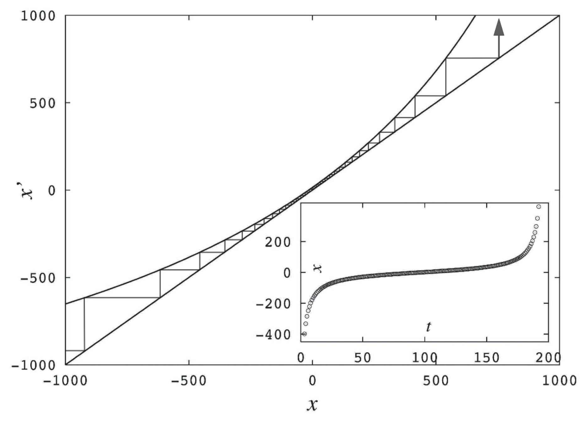
In Figs. 3 to 5 we illustrate the capability of this approach to reproduce quantitatively real data for ranking of eigenfactors (a measure of the overall value) of physics journals [9], industrial production growth rates by country [10], and per capita carbon dioxide emissions by country or region [11], respectively.
In the intermittency route out of chaos it is relevant to determine the duration of the so-called laminar episodes [6], i.e., the average time spent by the trajectories going through the “bottle neck” formed in the region where the map is closest to the line of unit slope. Naturally, the duration of the laminar episodes diverges at the tangent bifurcation when the Lyapunov exponent for separation of trajectories vanishes. Interestingly, it is this property of the nonlinear dynamics that translates into the finite-size () properties of the occurrence-rank function , that we have obtained without finding out the details of the departure of the basic distribution from the pure power-law . One more important result that follows from the analogy between nonlinear dynamics and the rank law is that the most common value for the degree of nonlinearity at tangency is , obtained when the map is analytic at with nonzero second derivative, and this implies , close to the values observed for most sets of real data.
5 Universality and uniqueness of data ranking
The steepest-descent approximation is central to statistical mechanics (and in a more general context to large deviation theory [13]). This property facilitates the evaluation in the thermodynamic limit of a partition function for one particular ensemble in terms of the partition function of another. Thermodynamically, this approximation relates to the Legendre transformation between the corresponding free energies or Massieu potentials where one variable is eliminated in favor of its conjugate [14]. As recalled above, the procedure consists of two steps, summation (or subtraction) of the product of the conjugate variables to (or from) the first potential to define the second, followed by use of the derivative of the first potential, or equation of state, to remove the undesired variable. This, of course, corresponds to the optimization involved in the steepest-descent method. For illustrative purposes we will assume here that the steepest-descent shortcut that underlies the second step in the Legendre transformation is also meaningful for .
In order to carry out the second step in the Legendre transform stated by Eq. (7) we need an explicit form for the function . It is evident that the form of this function is not unique and is determined by the particular set of data . For illustrative purposes we consider a finite set of data extracted from although a pure power law is not the correct distribution in this case. However, if the equivalent map Eq. (17) is very close to tangency and the data for the maximum rank, , is chosen such that its image in the map is to the left and near to its bottleneck mid-point, then is closely approximated by the power law. Under this approximation normalization of only yields . Suppose the available data, or the choice of the data collector, fixes the specific value of and the lowest and upper limits in Eq. (2) to be and , respectively. Therefore we have
| (18) |
, or
| (19) |
For example, a set of data about population of cities may be represented by (fifty representative city sizes), (one city with the largest population), and (one hundred cities with the smallest population considered). Eq. (19) is the required expression for to be used in the ‘steepest-descent condition’ or ‘equation of state’ Eq. (8). The result follows immediately, it is .
6 Summary and discussion
We have suggested here a novel thermodynamic, or statistical-mechanical, interpretation or understanding of the generalized laws of Benford and Zipf. The expressions for these laws, Eqs. (1) and (2) (or alternatively (4)) were derived in Ref. [4] under the basic assumption that the data sets obeyed by these laws are statistically well reproduced when extracted from a power law distribution . We remark here that the deviation from unity of the exponent implies a restricted access to the phase space for the data configurations that when enumerated produce the numbers . The restriction involves an accessible subset of this space with a scale invariant property, i.e., a fractal set, as implied by the power law . This viewpoint becomes evident when is seen to represent the probability distribution of equally probable configurations in the phase space for the data, and, consequently, suggests the definition of the generalized entropies in Eq. (6). It is important to clarify that the statistical-mechanical structure considered here and obtained from the usual via a scalar deformation parameter (represented by the power ) does not conform to that known as nonextensive statistics [15] [16]. Even though we define entropies or Massieu potentials with the use of the -logarithmic function and make use of its inverse, the -exponential, we do not require or implicate the optimization of any of these quantities via the use of the constraints employed in the nonextensive formalism or involve the use of the so-called escort distributions [16].
The ranking of real data habitually shows deviations from the Zipf’s power-law regime both for small and large rank that can be clearly observed in semi-log plots. As we have shown in Fig. 1 the generalized Zipf’s law given by Eq. (4) is capable of reproducing accurately the low rank deviation but not that for large rank as the power-law regime in this equation extends to . An upper bound for suggests finite-size effects inherent in real data. We have captured the nature of the upper bound for by first demonstrating a precise analogy between the expression for the ranking laws, Eqs. (3) and (4), and those for the dynamics at the transition to chaos via intermittency (the tangent bifurcation) in nonlinear maps of low dimensions. The finite-size effects in the ranking of data are seen to correspond to the shift off tangency in the map, so that the position of the upper bound for the rank is given by the duration of the laminar episodes of chaotic trajectories near the transition to regular behavior. Interestingly, the statistical-mechanical interpretation put forward for the generalized law of Zipf extends over to the critical dynamics of the transition to chaos via intermittency. While, on the practical side, data for the ranking of data for all is reproduced quantitatively by our formalism, as illustrated, respectively, in Figs. 3 to 5 for three specific examples: eigenfactor of physics journals [9], industrial production rates [10], and carbon emissions [11]. In agreement with empirical determinations the analogy implies that the most general value for the index is .
As it is generally well-known, a statistical-mechanical structure (shared by large deviation theory [13]) is built around the steepest-descent approximation and is expressed as the Legendre transform property that links different thermodynamic potentials. It involves an optimization condition or equation of state that relates conjugate variables. Only for illustrative purposes we have assumed that this structure extends to the deformed version (with one scalar parameter) we have considered here. In order to replicate the circumstances normally encountered in thermodynamics we have presented as an example the particular form taken by the function when the data in hand is bounded by the numbers and and fixes the largest rank . Then, the equation of state was determined and the variable eliminated in favor of , to obtain the ‘equilibrium’ value for . This exercise suggests that the universality of the laws is due to the general form of the incomplete Legendre transformation, while the expressions for the initial and transformed potentials are specific to the design of the data sample under consideration. The thermodynamic interpretation we have put forward may explain the ever presence of these phenomenological laws in a wide range of observations including very dissimilar situations. Finally, we comment that our arguments also apply to the topic of scale-free networks [17]. Since the degree distribution , the distribution for the number of links that connect one node to other nodes, describes essentially the ranking of nodes according to the number of links they possess, we can treat the data sets from where this distribution is phenomenologically obtained similarly to the data sets leading to Zipf’s law. Interestingly, for random link networks decays exponentially (), but for scale-free networks it is approximately power law ().
Acknowledgements
We recognize support from DGAPA-UNAM and CONACyT (Mexican agencies) and MEC (Spain). A.R. is grateful to the Grupo Interdisciplinar de Sistemas Complejos (GISC) for hospitality in Madrid.
References
- [1] G.K. Zipf, Human Behavior and the Principle of Least-Effort, (Addison-Wesley, 1949)
- [2] F. Benford, The Law of Anomalous Numbers, inProceedings of the American Philosophical Society 78 (4) (1938), p. 551.
- [3] See Johan Gerard van der Galien (2003-11-08) in http://en.wikipedia.org/wiki/Zipfs\_law
- [4] L. Pietronero, E. Tosatti, V. Tosatti, A. Vespignani, Physica A 293, 297 (2001).
- [5] G. Leech, P. Rayson, A. Wilson, Word Frequencies in Written and Spoken English: based on the British National Corpus, (Longman, London, 2001)
- [6] H. G. Schuster, Deterministic Chaos. An Introduction, 2nd Revised ed. (VCH, Weinheim, 1988).
- [7] F. Baldovin, A. Robledo, Europhys. Lett. 60, 518 (2002)
- [8] B. Hu, J. Rudnick, Phys. Rev. Lett. 48, 1645 (1982)
- [9] See subject category: Physics, year: 2007 in http://www.eigenfactor.org/index.php
- [10] See CIA World Factbook 2010 in https://www.cia.gov/library/publications/the-world-factbook/rankorder/2089rank.html
- [11] See International Energy Annual 2005 in http://www.photius.com/rankings/\\carbon\_footprint\_of\_countries\_per\_capita\_1980\_2005.html
- [12] C. Altamirano, A. Robledo, A., in Complex Sciences, LNICST Vol. 5 (Springer-Verlag, 2009), p. 2232
- [13] H. Touchette, Phys. Rep. 478, 1 (2009)
- [14] H. B. Callen, Thermodynamics and an Introduction to Themostatistics, 2nd edn. (John Wiley & Sons, New York, 1985)
- [15] C. Tsallis, J. Stat. Phys. 52, 479 (1988)
- [16] C. Tsallis, R. S. Mendes, A. R. Plastino, Physica A 261, 534 (1998)
- [17] R. Albert, A. Barabási, Rev. Mod. Phys. 74, 47 (2002)