Long-lived qubit from three spin-1/2 atoms
Abstract
A system of three spin-1/2 atoms allows the construction of a reference-frame-free (RFF) qubit in the subspace with total angular momentum . The RFF qubit stays coherent perfectly as long as the spins of the three atoms are affected homogeneously. The inhomogeneous evolution of the atoms causes decoherence, but this decoherence can be suppressed efficiently by applying a bias magnetic field of modest strength perpendicular to the plane of the atoms. The resulting lifetime of the RFF qubit can be many days, making RFF qubits of this kind promising candidates for quantum information storage units. Specifically, we examine the situation of three atoms trapped in a -laser-generated optical lattice and find that, with conservatively estimated parameters, a stored qubit maintains a fidelity of 0.9999 for two hours.
pacs
03.67.Pp, 03.65.Yz, 03.67.LxI Introduction
The processing of quantum information — be it for quantum communication, for quantum key distribution, or for quantum computation — requires the storage, manipulation, and retrieval of qubits that are carried by physical systems. This “hardware” can consist of selected well-controllable degrees of freedom of single photons, trapped ions, N-V centers in solids, or quantum dots, to name a few. All of them have advantages and disadvantages that make them well-fit for some purposes and unsuitable for others [1]. Practical applications that go beyond proof-of-principle experiments rely on qubits that are sufficiently robust for the task at hand.
For example, fault-tolerant quantum computation requires a gate fidelity that is very close to unity. Lack of control over the system, however, always gives rise to decoherence. The typical decoherence time for quantum dots, ions in a trap, or diamond N-V centers is in the order of microseconds or milliseconds, and a decoherence time of a few seconds is in reach of the current technologies [1]. This is still not quite sufficient for carrying out some complicated gate operations, nor for storage purposes [2].
We explore here a scheme to overcome the decoherence problem with reference-frame-free (RFF) qubits constructed from three spin-1/2 neutral atoms. These RFF qubits have a remarkably long lifetime — a NMR proof-of-principle experiment that employs three spin-1/2 nuclei is on record [3] — and the alignment of reference frames between observers, or the drift of frame between storage and read-out, is not an issue.
The said construction of RFF qubits from trios of spin-1/2 atoms was studied previously [4, 5]. These atoms are individually highly sensitive to magnetic stray fields, but their symmetric RFF states are completely insensitive as long as the stray field affects all three atoms in the same way [6]. Decoherence of the RFF qubit could, therefore, result from spatial inhomogeneities of the stray field. We investigate the effect of such inhomogeneities and demonstrate that the RFF qubits are highly robust: For typical experimental parameters, the magnetic stray fields are of no concern.
Rather, the lifetime of the RFF qubit is limited by the magnetic dipole-dipole interaction among the constituent atoms in conjunction with intrinsic imperfections of the experimental set-up. Our analysis, which uses conservatively estimated parameters and reasonable assumptions about experimental imperfections, shows that a stored qubit maintains a fidelity of 0.9999 or 0.999 for two or seven hours, respectively.
The outline of the paper is as follows. We first review the construction of the RFF qubit in Sec. II, followed by a qualitative discussion of possible causes of decoherence. In Sec. III, we analyze the robustness of the RFF qubit against decoherence under random stray magnetic fields and conclude that the stray fields are innocuous. We then consider, in Sec. IV, the inhomogeneous magnetic dipole fields of the partner atoms and find that, in view of unavoidable experimental imperfections, they are the dominating effect that limits the period for which quantum information can be stored. Section V briefly argues that the RFF system formed by three spin-1/2 constituents is more robust than the system formed by four spin-1/2 constituents. An experimental realization could use ultracold atoms in an optical potential of a suitable geometry [7, 8, 9, 10]; we mention one possibility of creating a potential of this kind in Sec. VI. We close with a Summary and Discussion.
II Construction of the RFF qubit
For a system of three spin-1/2 particles, the total spin of the system can be either 1/2 or 3/2. In the subspace, there are four states with different values; in the subspace, there are two different values, , with two states each, which we distinguish by the quantum number : with or .
We construct these four orthogonal basis kets in the sector by a variant of the procedure described in Ref. [5]. When denoting the Pauli vector operator for the th atom by , the total spin vector operator is given by
| (1) |
in units of . The lowering operator has the partner operators [11]
| (2) |
where is the lowering operator for the th atom, and is the basic cubic root of unity. We write for for brevity and choose the “” kets in accordance with
| (3) |
and an application of gives the corresponding “” kets,
| (4) |
with the outcomes
| (5) |
and
| (6) |
The arrows symbolize “spin up” and “spin down” in the -direction, so that in Eqs. (3) and (4). The kets have the usual properties as eigenstates of , namely
| (7) |
as one verifies immediately.
Since the eigenvalues of distinguish the and sectors, we can express the respective projectors in terms of ,
| (8) |
consistent with and . Alternatively, the projector onto the subspace with is given by
| (9) | |||||
where the latter expression is available either as a consequence of Eqs. (5) and (6) or of Eqs. (8) and (1).
The subspace and the subspace are both four-dimensional Hilbert spaces and, therefore, they can be regarded as tensor product spaces of two qubits, respectively. This is of no consequence for the sector, but it permits to write the sector as composed of a rotationally invariant signal qubit — the RFF qubit — and an idler qubit [5]: the kets of Eqs. (3)–(6) are labeled by the idler quantum number and the signal quantum number .
With the idler qubit in a maximally mixed state, the RFF state is identified by
| (10) |
where this tensor-product structure applies within the subspace with . We exhibit the statistical operator of the signal qubit alone,
| (11) |
by tracing over the idler qubit. The hermitian Pauli operators , , for the RFF qubit,
| (12) | |||||
are explicitly given by
| (13) |
These are clearly rotationally invariant and possess the algebraic properties of Pauli spin operators in the subspace, such as and .
Once the information is encoded in a RFF qubit (11), with the idler in the maximally mixed state as in Eq. (10) or in some other state, the information will be perfectly preserved as long as all three spin-1/2 atoms precess in unison. In the non-ideal circumstances of a real experimental situation, however, the interaction with the environment and the interactions among the physical carriers of the qubit could cause decoherence, because the atoms may be subject to torques of different strengths. Inevitably, there will be sources of noise over which the experimenter lacks control. It is our first objective to demonstrate that the information stored in the RFF qubit is preserved for a long time if magnetic stray fields with typical properties affect the carrier atoms.
III Magnetic stray fields
III.1 Noise model
The part of the Hamiltonian that describes the effect of the noisy magnetic field on the trio of atoms is given by
| (14) |
where is the Bohr magneton (if necessary multiplied by a gyromagnetic ratio) and is the randomly fluctuating magnetic stray field that acts on the th atom. The s vanish on average,
| (15) |
where the overline indicates the stochastic average. Since the atoms are close to each other, the fluctuations in the magnetic fields at the positions of the atoms are not independent but correlated. The dominant part of the noisy magnetic field is the same for all three atoms, and only a small part of the noise affects the atoms differently as a consequence of the nonzero gradient of the magnetic field. Upon denoting the gradient dyadic of the magnetic stray field by , we have
| (16) |
where is the position vector for the th atom, and is assumed to be independent of position within the small volume of relevance. This gradient component is the inhomogeneous noise that gives rise to decoherence of the RFF qubit, while the homogeneous noise is innocuous.
In the noise model considered, every component of the homogeneous stray field and every component of the gradient dyadic has a random gaussian distribution with a vanishing mean. Owing to the Maxwell’s equations, the gradient dyadic has to be symmetric and traceless:
| (17) |
It follows that the two-time correlation function of the field gradient has the form
| (18) | |||||
for any four vectors , , , and that pick out the components of , whereby is the variance of the gaussian distribution of the diagonal entries of , and is the decay constant for the temporal correlation. We note that the diagonal elements and the off-diagonal elements of the gradient matrix do not have the same variance:
| (19) | |||||
where and are two orthogonal unit vectors. The autocorrelation function for the diagonal components of is 4/3 times that of the off-diagonal components, while they have the same correlation time .
As a consequence of Eq. (18), the autocorrelation of the field difference of Eq. (16) is
| (20) | |||||
with . The correlation between the stray fields at the sites of the th atom and the th atom is then given by
| (21) |
where is the strength of the same-site correlation, as we recognize by a look at the version,
| (22) |
Consistency with Eq. (20) is established by using Eq. (21) four times on the right-hand side of
| (23) | |||||
Equations (15) and (21) define the noise model that we use in Sec. III.3 below to derive the master equation by which we then study the effect of the inhomogeneous magnetic stray fields on the RFF qubit in Sec. III.4, and on a single-atom qubit in Sec. III.5. The model is characterized by the three parameters , , and , which would have to be determined from experimental data when applying the model to an actual laboratory situation. Other noise models are conceivable, in particular if one wants to describe a specific noise source of known characteristics. The noise model of Eqs. (15) and (21) is generic, however, and quite suitable for the purpose at hand.
In an experimental realization of the three-atom RFF qubit, there will be nearby Helmholtz coils for the precise control of the magnetic field at the location of the atoms. Typically, these coils are about away and carry currents of about that are stabilized to or better [12]. Now, a current of at a distance of gives rise to a magnetic field of and a field gradient of . Not assuming any fortunate cancellation of the contributions from different coils, the values and are conservative estimates for these noise parameters. The temporal properties of the fluctuating currents tend to be dominated by the ubiquitous noise that the wires pick up, while high-frequency noise can be filtered out very efficiently, so that a correlation time of is a reasonable estimate [12]. We will use these numbers throughout the paper.
III.2 Lithium-6
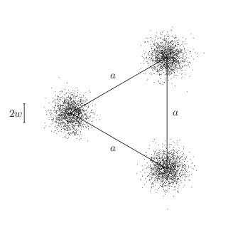
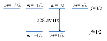
To be specific, but also mindful of possible experiments with two-dimensional confinement [13], we consider the situation of Fig. 1: Three 6Li atoms at the corners of an equilateral triangle, perhaps the sites of neighboring minima of an optical potential such as the one discussed below in Sec. V. Each 6Li atom is in the hyperfine ground state with , which is energetically below the hyperfine state by ; see Fig. 2.
We denote the electronic spin operator of the th atom by , with , so that the energy of the atom trio in an external homogeneous magnetic bias field is given by
| (24) |
where we take the value of for the gyromagnetic factor of the electron. With each atom confined to its ground state, this becomes
| (25) |
where is the gyromagnetic ratio and is the total atomic angular momentum in the present context; the magnetic moment of the spin-1 nucleus is ignored. As indicated, here we identify the Pauli operators of Eqs. (1), (9), (13), or (14).
We choose the bias field in the -direction, perpendicular to the -plane in which the atoms are located, , and express its strength in terms of the circular frequency : ; then
| (26) |
The coupling of the and the multiplets by the bias field is ignored, which is permissible if the field is weak on the scale set by the energy difference, that is: . For example, this condition is met for the modest field strength of , when is a thousandth of a percent of the transition frequency, and transition probabilities are of the order of .
We need the bias field to fight the “internal magnetic pollution” that originates in the magnetic dipole-dipole interaction between the spin-1/2 atoms. In terms of the electronic spin operators, this interaction energy is [14]
| (27) |
where is the common distance between the atoms at the corners of the equilateral triangle, is the unit vector that points from the th to the th atom, and the summation is over the three pairs. As in the transition from Eq. (24) to Eq. (25), the restriction to the ground state amounts to the replacement
| (28) |
which turns Eq. (27) into
| (29) |
with
| (30) |
For a distance of (see Sec. VI below), we have , smaller than by a factor of , so that the transitions induced by are completely suppressed in the presence of a bias field. Therefore, only the part of that commutes with of Eq. (26) is relevant, and we arrive at
| (31) |
as the effective Hamiltonian for the magnetic dipole-dipole interaction among the atoms. Note that this vanishes in the sector where the signal and idler qubits reside.
The combined effective Hamiltonian
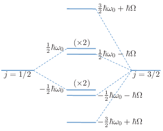
| (32) |
has the non-degenerate eigenvalues and in the sector, and the two-fold eigenvalues in the sector; see Fig. 3. The energy differences correspond to transition frequencies of about , which are in the few-kHz range, and to transition frequency , which is , if we continue to use the numbers found above. There is a clear separation of time scales, then, and noise with a correlation time in the order of — which we regard as a typical number, see above — would not be able to induce transitions between the states separated by several while it will mix the states that are separated by only or not at all.
There are, of course, stray fields in the radio frequency range but their sources (the radio stations) are far away so that the gradient parameter is extremely small, and noise of this kind is of no concern. By contrast, noise originating in nearby sources — current carrying wires in the vicinity of the laboratory, say — is relevant.
III.3 Master equation
In view of this separation of time scales — very fast -oscillations and very slow -oscillations on the scale set by the correlation time of the random stray field — we can use master equation techniques to account for the net effect of the noise. For the purpose of deriving the Lindblad operators of the master equation, we put of Eq. (32) aside and use an interaction picture in which the fast -oscillations of are transformed away. The statistical operator in this interaction picture, denoted by , then obeys the von Neumann equation of motion
| (33) |
with
| (34) | |||||
where the replacement accounts for the gyromagnetic ratio that we first met in the transition from Eq. (24) to Eq. (25).
The unitary evolution operator links to the initial statistical operator ,
| (35) |
We solve the Lippmann–Schwinger equation
| (36) |
to second order in ,
| (37) |
where the hermitian phases and are given by
| (38) |
To second order in , then, we have
| (39) | |||||
and the stochastic averaging of Sec. III.1 turns this into
| (40) | |||||
where and the initial statistical operator is not affected by the averaging or the transition to the interaction picture: . Note that follows from Eq. (15).
We take a closer look at the “sandwich term” in the double commutator,
| (41) |
Here, is much longer than the correlation time of the noise, , so that there are very many cycles of the -oscillation in a short -interval. Therefore, the rapidly oscillating terms in do not contribute to the -integration and the replacement
| (42) |
is permissible; and likewise for . This “rotating-wave approximation” takes us to
| (43) | |||||
after using Eq. (21) for , , and . For , the remaining double integral equals , and we arrive at
| (44) |
with the time constants
| (45) |
and
| (46) |
Since , we have , and the numbers of Sec. III.2, that is: and , give — an amazingly long time.
The replacement of Eq. (42) gives a vanishing commutator in the double integral for in Eq. (38), so that in Eq. (40). In summary, then, we have
| (47) |
with the Lindblad operator given by
| (48) |
and the master equation in the interaction picture is simply
| (49) |
Upon getting out of the interaction picture, and re-introducing the slow -oscillations of , this gives us the master equation
| (50) |
for the evolution of the coarse-grain, stochastically averaged, statistical operator .
We note in passing that this master equation could alternatively be derived with standard textbook methods, such as those that proceed from the Redfield equation, here:
| (51) |
and invoke the Born–Markov approximation and the rotating-wave approximation to arrive at Eq. (49). For details of this procedure, see section 3.2 in Ref. [15], for example.
In view of the diagonal form of the Lindblad operator in Eq. (48), the expectation value of an observable obeys the differential equation
| (52) |
For observables that commute with , which is the case for all operators related to the signal qubit, only the part of and the -term of matter, and then the simpler equation
| (53) |
applies. In particular we have
| (54) |
for all functions of . The product
| (55) |
states the relative size of the time constants in Eq. (53). It depends rather strongly on the distance between the atoms; we have for the values used earlier (, , ).
III.4 Time dependence of RFF-qubit variables
By making use of Eq. (53), we can now calculate , the probability of finding the three-atom system in the sector at time , and the time-dependent expectation values of the RFF-qubit Pauli operators of Eqs. (13) and (12). The outcome is
| (56) |
if the system is initially in the sector, where the idler and signal qubits reside. The expressions for and are exact solutions of the respective versions of Eq. (53), and the result for is an approximation that neglects terms of relative size .
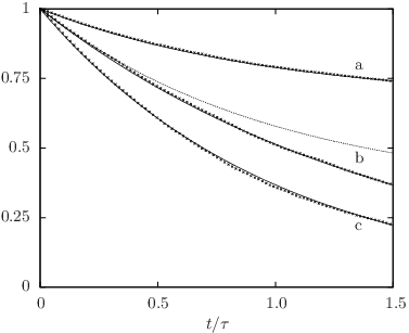
Supporting evidence is provided by numerical simulations [16]. These are done by generating a RFF state at initial time and letting the state evolve with stochastic random noisy magnetic fields on the three atoms. All components of the noise are generated randomly at each time step from a gaussian distribution, and the Maxwell’s equations are strictly imposed on the magnetic fields. Figure 4 shows both the analytical and the numerical results of the evolution of the RFF qubit for an arbitrary initial RFF state. We note that there is very good agreement between the results of the simulation and the analytical solution of the master equation.
Quantum information stored in the RFF qubit is degraded substantially only after a good fraction of has elapsed. But since is more than , we conclude that the effect of the inhomogeneous magnetic stray fields is of absolutely no concern. Put differently, the experimenter need not take special measures to suppress the stray fields.
III.5 Decoherence of a single-atom qubit
If — rather than making good use of the three-atom RFF signal qubit — one encoded quantum information into the ground state of a single 6Li atom, the effect of the random magnetic stray field would be described by the single-atom master equation
| (57) |
with
| (58) |
The resulting time-dependent expectation values are
| (59) |
so that the quantum information can be stored for a fraction of time .
The bias field stabilizes the component: It separates the spin-up and spin-down states in energy by and so prevents transitions between them — this is, of course, the essence of the rotating-wave approximation of Eq. (42). Therefore, one could encode a classical bit in a single spin-1/2 atom and protect it from the stray magnetic field. [17]
Without the bias field, the master equation
| (60) |
applies. Its solution
| (61) |
shows that the state decays toward the completely mixed state with a life time of . It follows that, in addition to preserving the component, the bias field also slows down the decay of the and components by a factor of two.
For the example used in Sec. III.1 — a fluctuating current in a wire at a distance of — we have and obtain . Even for the very large value of found above, , the lifetime of the single-atom qubit is quite short: . Clearly, the well-protected RFF qubit of the three-atom system has an advantage over the unprotected single-atom qubit: The stray fields, which are of no concern for the RFF qubit, have a devastating effect on the single-atom qubit.
More relevant than the lifetime is the duration of the initial period of high fidelity. We recall that the fidelity of two single-qubit states, specified by their respective Pauli vectors, is given by
| (62) |
For the fidelity between the initial qubit state and the state at later time , we have the lower bound
| (63) |
so that a fidelity of, say, 0.999 is only guaranteed for a fraction of a millisecond. By contrast, the RFF qubit would have a fidelity of 0.9999 or better for several months if nothing mattered except for the magnetic stray field.
We note that the ratio of and is solely determined by the comparison of the distance between the atoms and the distance of the atoms from the source of the noise, for which we have been using and , respectively, implying . Therefore, the conclusion that holds irrespective of the actual physical process that generates the stray magnetic field as long as the noise source is half a meter away.
IV Dipole-dipole interaction
Two assumptions of ideal geometry enter the derivation of the effective Hamiltonian for the dipole-dipole interaction in Eq. (31): That the atoms are located at the corners of a perfect equilateral triangle; and that the bias field is exactly perpendicular to the plane of the atoms. Let us now consider the consequences of imperfections on both counts.
IV.1 Center-of-mass probability distribution
As illustrated by the probability clouds in Fig. 1, the atoms do not have definite positions but rather probability distributions for their centers of mass, given by the ground-state wave functions of the trapping potentials. We assume that, for the purpose at hand, the respective trapping potentials are reasonably well approximated by isotropic harmonic oscillator potentials, so that each atom has a gaussian probability distribution,
| (64) |
where is the position of the trap center and is the width of the gaussian. The oscillator frequency of the trap is related to and the mass of the atom by
| (65) |
which is obtained by fitting the potential around the bottom of the trap to a harmonic-oscillator potential. For the potential of Sec. VI below, , so that the width of the gaussian wave function is . Accordingly, here, earlier in Fig. 1, and in what follows, we take the width to be about one-twelfth of the distance between the atoms.
When comparing the restoring force of the oscillator potential, , with the dipole forces exerted by the partner atoms, , we find that the balance of forces would shift the equilibrium position by an amount of the order of
| (66) |
which is a completely negligible effect. We also note that, depending on the joint spin state of the three atoms, the shift is in different directions, and the center-of-mass degrees of freedom get entangled with the spin degrees of freedom but, since the shift is such a tiny fraction of the position spread , this entanglement is so weak that it can be safely ignored. As a consequence, the center-of-mass motion is decoupled from the dynamics of the spins, and probability distributions as in Eq. (64) apply to the atoms at all times.
The total statistical operator for the three-atom system is then the product of the spin factor of Sec. III.3 and a static center-of-mass factor . The von Neumann equation for is obtained by tracing over the center-of-mass variables,
| (67) |
where is the total Hamiltonian. Of its four terms, the dipole-dipole interaction energy and the noise part involve both spin variables and center-of-mass variables. In view of the lesson learned in Sec. III, however, there is no need to deal with in detail.
We consider the center-of-mass average of the contribution from atoms 1 and 2 to ,
where is the vector from the trap center for atom 1 to the trap center for atom 2. Allowing for different widths of the two gaussians, the integration yields
| (69) |
with the standard error function . Its asymptotic form
| (70) |
tells us that the right hand side of Eq. (69) differs from by a term of relative size for . It follows that
| (71) |
in the present context, which is exactly the term in Eq. (29), and the center-of-mass probability distribution is of no further concern.
IV.2 Non-ideal geometry
But we need to account for the unavoidable imperfections of any experimental realization: The triangle formed by the trap centers for the tree atoms is not exactly equilateral, and the plane of the actual triangle is not exactly perpendicular to the -axis defined by the bias field.
First, with denoting the distance between the th and the th trap center, we define the average distance by means of
| (72) |
and measure the deviation of from by the small parameter ,
| (73) |
This average value is used in Eq. (30) to determine the dipole-dipole coupling strength , and we have
| (74) |
instead of Eq. (29), where denotes the unit dyadic. If the atoms are indeed trapped in the minima of an optical potential, is achievable without resorting to extreme measures [18].
Second, nonzero -components of the unit vectors require
| (75) |
for the step from Eq. (29) to Eq. (31). Misalignments that exceed can be avoided with standard experimental techniques [18], so that is a conservative estimate.
The combined effect of both imperfections is a modification of , such that
| (76) |
with
| (77) |
rather than the version of Eq. (31). The relative size of the imperfections is measured by
| (78) |
wherein, for the values of and above, the three terms are of the order , , and , respectively, and the contribution dominates.
We note in passing that the imperfection parameters and the dot products that appear on the right-hand side of Eq. (78) are not independent of each other. Rather, the triangle condition imposes the restriction
| (79) |
where the summation over the pairs is cyclic, that is: , , and .
The operator vanishes in the sector,
| (80) |
and there are no first-order contributions from the -term to the evolution of the RFF qubit. It follows that, during the initial period of high fidelity, the geometrical imperfections contribute in second-order of the small parameters.
IV.3 Time dependence of RFF-qubit variables
For a quantitative analysis, we employ the master equation that results when Eq. (50) is modified in accordance with the observations made here and above,
| (81) | |||||
where we put , in the Lindblad operator of Eq. (48). While the double-commutator term leads to the fast decay of single-atom spin coherence, as we saw above in Sec. III.5, it is of no consequence for the RFF qubit because all RFF observables as well as their commutators with commute with . It follows further that the expectation value of a RFF variable , with the three-atom system initially prepared in the sector, is given by
| (82) |
with
| (83) | |||||
where
for
| (87) |
For in Eq. (78), we have first and then and . Accordingly, is the sum of a long-period oscillation with a large amplitude and a short-period oscillation with a small amplitude; see Fig. 5.
The resulting time-dependent expectation values of the RFF observables are
| (88) |
with
| (89) |
Equations (88) contain all information about the state of the signal qubit in the course of time. We use them to evaluate the purity of the signal-qubit state at time and its fidelity with the initial signal-qubit state.
The purity of the signal-qubit state is quantified by the squared length of its Pauli vector,
| (90) | |||||
so that an initially pure signal-qubit state, , remains pure. When the initial state is mixed, , both and are possible, depending on the relative size of and . Specifically, we have
| (91) |
and .
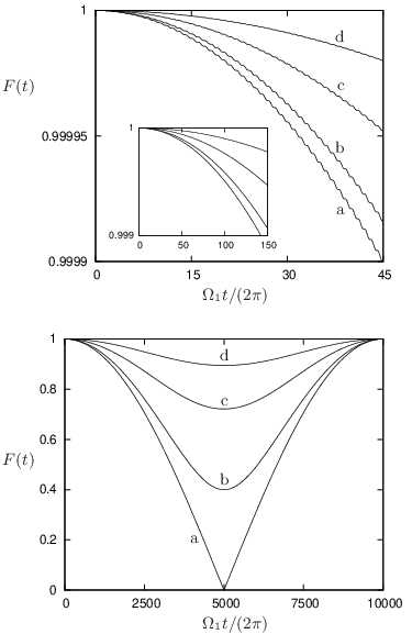
The fidelity of the signal-qubit state at the later time with the initial state is given by
| (92) | |||||
It is bounded from below by
| (93) |
where the equal sign holds for if, for example, and . For and , this bound is
| (94) |
where the ellipsis stands for terms of order . This two-term approximation serves all practical purposes for . The fidelity is assuredly very high during the early period dominated by the small-amplitude oscillations with frequency : We have or better for 45 periods of the fast oscillations, and or better for 140 periods, when . These matters are illustrated in Fig. 5.
IV.4 Compensating for triangle distortions
In Secs. IV.2 and IV.3 we regarded the imperfection parameters and as resulting from the lack of perfect control over the apparatus, and their values would not be known with high precision. Suppose, however, that the experimenter has diagnosed the set-up and knows the actual shape of the triangle quite well while having very precise control over the direction of the magnetic bias field. She can then attempt to adjust the bias field such that the three s of Eq. (78) are equal, with the consequence that in Eq. (87) and in Eq. (IV.3). We do not discuss this matter in further detail and are content with mentioning that, for small values of the s, a bias-field direction with
| (95) |
achieves this, where the approximation neglects terms of second and higher order in the s. With this compensation for the imperfections in the shape of the triangle by a judicious tilt of the bias field, the ratio can be reduced by much, with a corresponding lengthening of the initial period of high fidelity.
V RFF qubit from four spin-1/2 atoms
An alternative construction of a RFF qubit uses four spin-1/2 atoms and their two-dimensional subspace with . A pure state of the RFF qubit is then realized by a pure state of the four-atom system, and decay results from leakage to the sectors with and , which are nine-dimensional and five-dimensional, respectively. By contrast, a pure state of the three–spin-1/2–atom RFF qubit corresponds to a mixed state of the three-atom system with leakage into the space of the idler qubit and into the sector. Clearly, the two constructions of the RFF qubit are substantially different.
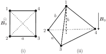
For comparison with the two-dimensional equilateral triangular configuration of three atoms, let us consider four atoms located at the corners of a square; see Fig. 6(i). The system is stabilized with a bias magnetic field perpendicular to the plane of atoms to reduce the decoherence due to the internal pollution from the dipole-dipole interactions. The distance between the two diagonal pairs of atoms is times larger than the distance between the four pairs at the sides. Thus, the dipole-dipole interaction is unbalanced between all pairs and it cannot be made rotationally invariant by the bias magnetic field. Explicitly, the effective dipole-dipole interaction is here given by
| (96) | |||||
with as in Eq. (30). For the same reasons as in the three-atom case, the stray magnetic field is of no concern, and the system evolves unitarily
| (97) |
The projector onto the subspace of the four-atom RFF qubit is given by
| (98) |
where the s are the singlet state between th and th constituents,
| (99) |
for and .
The effective dipole-dipole Hamiltonian has the structure of Eq. (76), with the operator now given by
| (100) |
where accounts for the relative reduction in the strength of the dipole-dipole interaction for the two diagonal atom pairs. Moreover, Eq. (82) continues to apply for the expectation value of a RFF operator , with the four-atom system initially prepared in the sector. Thereby, the effective unitary evolution operator is now
| (101) | |||||
where , , and are the RFF Pauli operators for the four-atom system as defined in Eqs. (25) of Ref. [5], and is exactly of the form in Eq. (IV.3) with and replaced by
| (102) |
which have a ratio of , very different from the ratio of in Eqs. (IV.3) and (87).
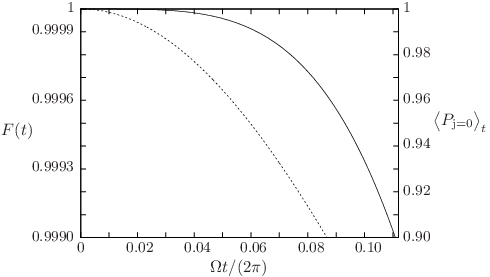
The expectation values of the RFF operators in the sector can be obtained analytically, in particular for the expectation value and the RFF qubit fidelity , for which the obvious analogs of in Eq. (88) and in Eq. (92) apply. With the four-atom version of , the lower bound on of Eq. (93) is valid, and we also have . Both lower bounds are shown in Fig. 7 for the high-fidelity period of . We have a fidelity of 0.9999 or better for and 0.999 or better for .
Note, in particular, the substantial probability of losing the four-atom RFF qubit: After the lapse of , there is a chance of more than 10% that the four-atom system has left the sector. This is a consequence of the rather small ratio. By contrast, for the three-atom qubit with , the persistence probability is never less than 0.9996.
The dipole-dipole coupling strength is proportional to , where is the length of the sides of the square. If we use laser beams with the same wavelengths as used for the three-atom system in Sec. VI to construct the potential for four atoms in a square geometry, the inter-atomic distance is and Eq. (30) gives . It follows that we can guarantee for about four seconds and for about seven seconds. This shows that even with a perfect square geometry, the RFF state constructed from four spin-1/2 atoms decays about 2000 times faster than the qubit constructed from three spin-1/2 atoms in an imperfect equilateral triangle configuration.
The imbalance in the dipole-dipole interaction strength between the pairs of atoms could be removed by using the three-dimensional pyramidal configuration of Fig. 6(ii). To fight against the internal magnetic pollution we apply a bias magnetic field perpendicular to the plane of three of the atoms which are arranged in an equilateral triangle, with the fourth atom above the center of the triangle. By adjusting the height of the pyramid such that the ratio between the atomic distances is , a rotationally invariant effective dipole-dipole potential is obtained. The lifetime of the RFF qubit for this four-atom geometry is comparable to the lifetime of the RFF qubit constructed from three atoms in the equilateral-triangle configuration examined in the previous sections. But the practical realization of the peculiar pyramidal arrangement, a distorted tetrahedron with reduced height, is much more challenging than the equilateral triangle.
Clearly, there is no advantage in using the RFF qubits made from four atoms over the RFF qubits made from three atoms. Rather, the simpler three-atom system is preferable.
VI Structure of the optical lattice
One kind of optical lattices that could be used is a modification of the Kagome lattice, where we have an equilateral triangular lattice of which every site is formed by three spin-1/2 atoms arranged in a small equilateral triangle. A possible physical construction of such a lattice is to use two sets of three coplanar coherent laser beams and the angle between the beams within each coherent set is . By arranging them in the configuration shown in Fig. 8 and adjusting the phases, an optical trapping potential with the contour plot shown in Fig. 9 can be produced. For the potential presented in Fig. 9, we chose to keep the phases of the set of beams with the longer wavelength to be the same and the phases for the other three beams with the shorter wavelength are , , and , but this choice of phases is not unique.
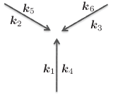
Under the joint consideration of being able to address each RFF qubit individually, of the necessity of high laser intensity to trap the 6Li atoms, and of the requirement of a low probability that the atoms scatter photons from the trapping lasers, we propose to use the laser, from which the desired wavelengths can be generated by frequency doubling (or tripling) in nonlinear media. lasers with wavelength 10.6m are widely used and a high beam intensity is routinely achieved, and optical trapping of 6Li is reported [19]. We can thus have and for the wavelengths in Fig. 8. For the produced lattice the atomic distance between atoms within the trio forming one RFF qubit is nm and the distance between the RFF qubits is m. The potential strength associated with the low-frequency laser is four times that of the high-frequency laser for the example of the potential given in this section.
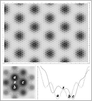
The recoil temperature of the (or ) line of 6Li is . To have an estimation of the trapping frequency, the function of the potential at the minima is fitted with a spherically symmetric harmonic potential. With the ratio between the laser intensity and the reduced saturation intensity , the frequency of the harmonic potential is about . The energy separation of the first excited state and the ground state of the harmonic potential is given by (), which is about five times the recoil energy. The polarizability of 6Li is , which yields a scattering rate below at this intensity, corresponding to a scattering time of more than for one photon per atom. Consequently, the recoil heating is negligible. Upon assigning a gaussian profile to the center-of-mass wave function of the atoms, the spread of the wave function is estimated to be for the trapping frequency above.
The depth of the optical trap is roughly , corresponding to a temperature of about and more than twenty times the recoil energy. The required intensity of the laser is about and for the laser it is about .
The numbers given above for the trap are for the sample potential presented here, which serves the purpose of demonstrating that such a lattice can be had. The properties of the trapping potential depend on the laser intensities and . Other methods for making an array of atomic trios are conceivable. This is a hardware issue and all details are determined by the experimental set-up at hand.
VII Summary and discussion
VII.1 Summary
We studied the effect of stochastic magnetic stray fields on the RFF qubit made from three spin-1/2 atoms and found that the RFF qubit decoheres very slowly although the spin states of the individual atoms decay very quickly. The only coupling of the spin-1/2 atoms to the environment is through their magnetic dipole moments, so that magnetic stray fields give rise to uncontrolled changes of the quantum state of the atoms. The long lifetime of the RFF qubit results from its insensitivity to the over-all magnetic field and its fluctuations because they affect all three atoms equally and, therefore, do not affect the RFF qubit at all. Decoherence of the RFF qubit originates in spatial variations of the magnetic field, but they are subject to the constraints imposed by the Maxwell’s equations. For parameter values that are typical for experimental situations, we find that the RFF qubit can maintain a very high fidelity for months — if the magnetic stray field is the only source of decoherence.
We then analyzed the effect of the dipole-dipole interactions among the three atoms and imperfections in the geometry of the trapped atoms. We found that the inter-atomic interactions bring more decoherence to the RFF qubit than the fluctuating magnetic stray fields, although the dipole-dipole interaction itself is a unitary process. Nevertheless, the RFF qubit states were shown to be very robust within the parameter regime and under our assumptions. As an example, we showed that the period of high fidelity, say , with respect to the initial state is roughly two hours.
VII.2 Assumptions
Let us review the assumptions that we used to derive the result and discuss their validity.
We have assumed that the atoms are trapped in the deep optical lattice at very low temperature so that their center-of-mass motions are negligible. One example for such a desired optical lattice, created by standard laser techniques, was presented in Sec. VI. We estimated, in Sec. IV.1, the effect of the center-of-mass motions and found that it is much smaller (i.e., ) than the effect of the dipole-dipole interactions for the optical lattice considered.
The most challenging element seems to be to maintain the stable lasers for the optical lattice in order to observe the long-time evolution of the RFF qubit. In a real experiment the collisions with rest-gas atoms are also inevitable and they may very well limit the lifetime of the RFF qubit in practice. We note that drifts of the lasers in time would not spoil the long lifetime as long as all lasers are locked in phase. This is because the time scale of these parameter changes is much slower and hence all atoms follow the optical lattice adiabatically.
The noise model employed in this study is divided into two types. One is a fluctuating magnetic stray field arising from unavoidable imperfections in the surrounding apparatuses such as the Helmholtz coils, electric wires, and so on. The Helmholtz coils used to generate the homogenous bias magnetic field are identified as the major source for the noise of this kind. Other possible fluctuating magnetic fields are much smaller than this and less inhomogeneous as the respective sources are farther away. We then linearized these fluctuating fields around the homogeneous bias field to analyze the decoherence for the RFF qubit in Secs. III.1 and III.3.
The other type of noise is due the magnetic dipole-dipole interaction among the three atoms. We have shown that these inter-atomic interactions are a major source of decoherence for the RFF qubit when imperfections of the experimental set-up are taken into account. In Secs. IV.2 and IV.3, we accounted for deviations from the ideal equilateral triangle configuration of the three atoms as well as a misalignment of the magnetic bias field and found that such insufficiencies still allow for a very long lifetime of the RFF qubit. In fact, we observed that imperfections in the geometry of the three atoms could be compensated for by adjusting the direction of the bias magnetic field, provided that the experimenter has sufficient control over the relevant parameters.
We should not forget to mention that the rotating-wave approximation was used, for example, when analyzing the effect of fluctuating magnetic stray fields. This approximation is valid within the energy scale of our set-up, where a probability for a non-resonant transition is very small. The numerical study without the rotating-wave approximation also supports the validity of our master-equation analysis.
All these results are, of course, derived with the assumption that the parameters used in this study are well controlled with a certain precision. We however took rather conservative numbers for these parameters so that we can estimate a realistic lifetime of the RFF qubit. This also leaves some room for improving the lifetime of the RFF qubit in further studies.
VII.3 Alternatives
In the scheme presented here, the RFF state is made from three spin-1/2 atoms. But this is not the only way to construct RFF qubits. We can equally well use three identical atoms of any non-zero ground-state spin , where the RFF signal qubit lives in the subspace of total angular momentum , which has two states for each value. The idler space is then -dimensional. Analogously, RFF qutrits can be constructed in the sector of total angular momentum from four identical atoms with ground state spin . Such alternative constructions offer considerable flexibility in choosing the isotope for a practical implementation.
As we mentioned in Sec. V, other geometries and four atoms are not better than the case of three atoms in the equilateral triangle, but they are still good for the purpose of storing quantum information. For example, three or four atoms on a line, with the bias field in the right direction, could be an easier choice for a trapped-ion experiment. Likewise, physical systems other than cold atoms should in principle give a long lifetime if information is encoded in the RFF subsystem. There are advantages and disadvantages depending upon the physical system one chooses. All these are largely unexplored territories that need further surveying.
VII.4 Outlook
Having thus shown how to construct robust units for storing quantum information, the problems of how to encode and read out the information, and how to process it in such a set-up, need to be addressed. We will report progress on this front in due course.
Acknowledgements.
Centre for Quantum Technologies (CQT) is a Research Centre of Excellence funded by Ministry of Education and National Research Foundation of Singapore. N.L. would like to thank the Studienstiftung des deutschen Volkes for financial support. J.S. is supported by NICT and MEXT. Both N.L. and J.S. would like to thank CQT for the kind hospitality. H.R. wishes to thank Kae Nemoto and the National Institute of Informatics for their warm hospitality. Both H.R. and B.-G.E. thank Hans Briegel and the Institute for Quantum Optics and Quantum Information for their warm hospitality. We gratefully acknowledge Ng Hui Khoon’s enlightening comments and friendly discussions.References
- [1] T.D. Ladd, F. Jelezko, R. Laflamme, Y. Nakamura, C. Monroe, and J.L. O’Brien, Nature (London)464, 45 (2010).
- [2] C. Simon, M. Afzelius, J. Appel, A.B. de la Giroday, S.J. Dewhurst, N. Gisin, C.Y. Hu, F. Jelezko, S. Kröll, J.H. Müller, J. Nunn, E.S. Polzik, J.G. Rarity, H. De Riedmatten, W. Rosenfeld, A.J. Shields, N. Sköld, R.M. Stevenson, R. Thew, I.A. Walmsley, M.C. Weber, H. Weinfurter, J. Wrachtrup, and R.J. Young, Eur. Phys. J. D 58, 1 (2010).
- [3] L. Viola, E.M. Fortunato, M.A. Pravia, E. Knill, R. Laflamme, and D.G. Cory, Science 293, 2059 (2001).
- [4] S.D. Bartlett, T. Rudolph, and R.W. Spekkens, Rev. Mod. Phys. 79, 555 (2007).
- [5] J. Suzuki, G.N.M. Tabia, and B.-G. Englert, Phys. Rev. A78, 052328 (2008).
- [6] D.A. Lidar and K.B. Whaley, Lect. Notes Phys. 622, 83 (2003).
- [7] D. Jaksch, C. Bruder, J.I. Cirac, C.W. Gardiner, and P. Zoller, Phys. Rev. Lett. 81, 3108 (1998).
- [8] M. Köhl, H. Moritz, T. Stöferle, K. Günter, and T. Esslinger, Phys. Rev. Lett. 94, 080403 (2005).
- [9] J. Cho, Phys. Rev. Lett. 99, 020502 (2007).
- [10] S. Trotzky, P. Cheinet, S. Fölling, M. Feld, U. Schnorrberger, A.M. Rey, A. Polkovnikov, E.A. Demler, M.D. Lukin, and I. Bloch, Science 319, 295 (2008).
- [11] The correspondence with the conventions of Ref. [5] is the following: What is here, is there; the labels here are there; and the operators and here are and there. For the record we note that an inadvertent interchange between and happened in the transition from Sec. III to Sec. IV A in [5].
- [12] G. Maslennikov, private communication (2010).
- [13] K.L. Lee, B. Grémaud, R. Han, B.-G. Englert, and C. Miniatura, Phys. Rev. A80, 043411 (2009).
- [14] There is no need, here or later in Sec. IV.1, to include the contact term .
- [15] H.-P. Breuer and F. Petruccione, The theory of open quantum systems (Oxford University Press, Oxford and New York, 2002).
- [16] N. Lörch, A study of open quantum systems (Diplomarbeit: Universität Heidelberg, 2010).
- [17] When using two atoms, the bias field separates the and states from the and states, which have approximately the same energy and can be used for the storage of a qubit. A life time of several seconds was achieved in an ion-trap experiment [20].
- [18] D. Wilkowski, private communication (2010).
- [19] K.M. O’Hara, S.R. Granade, M.E. Gehm, T.A. Savard, S. Bali, C. Freed, and J.E. Thomas, Phys. Rev. Lett. 82, 4204 (1999).
- [20] C. Langer, R. Ozeri, J.D. Jost, J. Chiaverini, B. DeMarco, A. Ben-Kish, R.B. Blakestad, J. Britton, D.B. Hume, W.M. Itano, D. Leibfried, R. Reichle, T. Rosenband, T. Schaetz, P.O. Schmidt, and D.J. Wineland, Phys. Rev. Lett. 95, 060502 (2005).