Invariants of tangles with flat connections in their complements

Let $I\equiv[0,1]$ be the closed unit interval. A geometric tangle $t\subset{{\mathbb{R}}^{2}}\times I$ is the image of a smooth embedding $\underbrace{I\sqcup\ldots\sqcup I}_{k\ \mathrm{times}}\sqcup\underbrace{S^{1}\sqcup\ldots\sqcup S^{1}}_{l\ \mathrm{times}}\to{\mathbb{R}}^{2}\times I$ with oriented components such that $\partial t\subset{{\mathbb{R}}^{2}}\times\partial I$, and $t$ intersects the boundary ${\mathbb{R}}^{2}\times\partial I$ perpendicularly. We have $\partial t=\partial_{+}t\sqcup\partial_{-}t$ where $\partial_{+}t=({\mathbb{R}}^{2}\times\{1\})\cap\partial t$ and $\partial_{-}t=({\mathbb{R}}^{2}\times\{0\})\cap\partial t$. The geometric tangle $t$ is called standard if $\partial_{+}t=\{(0,1,1),(0,2,1)\dots(0,n,1)\}$ and $\partial_{-}t=\{(0,1,0),(0,2,0)\dots(0,m,0)\}$ for some $n,m\in{\mathbb{Z}}_{>0}$. We will say that such tangle has type $(m,n)$.

Denote by $D_{t}$ the image of $t$ under the projection

together with the additional information at each self-crossing point about underpassing and overpassing segments. The projection $D_{t}$ is called regular if its only singularities are double points at which the images of the corresponding components of $t$ intersect transversally. The ambient isotopy class of a regular projection $D_{t}$ is called a diagram of the tangle $t$. When it is not confusing we will use the same notation $D_{t}$ for diagrams and regular projections.

The diagram of a tangle can be regarded as the isotopy class of a smooth embedding of a graph with four-valent vertices of two types and one-valent vertices. These are the double points and the boundary points, respectively. The edges of the graph are the segments running between the vertices. A vertex of $D_{t}$ is called positive if it is a double point and the angle between upper and lower components is positive. If the angle is negative, the vertex is called negative, see Fig. 1. Each such embedding is always a diagram of some tangle. Two diagrams are called Reidemeister equivalent if one can be obtained from another by a finite sequence of Reidemeister moves (see Figs 2–4).

A tangle is the isotopy class of a geometric tangle. Tangles are in bijection with Reidemeister classes of diagrams.

A geometric framing of a geometric tangle $t$ is a continuous nonsingular section of the normal bundle to $t$. A framing of a tangle is the isotopy class of a geometric framing. A framing is standard if it is parallel to the $x$-axis at $\partial_{\pm}t$ with positive projection to this axis. It is clear that every framed geometric tangle with such framing at the boundary is isotopically equivalent to a framed geometric tangle with the framing parallel to $x$-axis. Framed tangle is the isotopy class of a framed geometric tangle with the standard framing.

Two diagrams of tangles are called framed Reidemeister equivalent if they are connected by a sequence of moves in Figs 2, 3, 5.

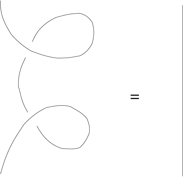
Framed Reidemeister classes of diagrams are in bijection with the framed tangles.

Let $E$ be a trivial principal $G$-bundle over ${\mathbb{R}}^{2}\times I$ and $A_{t}\in\Omega^{1}({\mathbb{R}}^{2}\times I\backslash t,{\mathfrak{g}})$ be the 1-form representing a flat connection in $E$ over the complement to a standard geometric framed tangle $t$ of type $(m,n)$. The corresponding parallel transport operators along paths give an equivalent description of the flat connection as a representation of the fundamental groupoid of $({\mathbb{R}}^{2}\times I)\backslash t$ in $G$. ^††margin: $\leftarrow$ *

Let $E_{m}$ be a trivial principal $G$-bundle over ${\mathbb{R}}^{2}$, and $\alpha$ be the ${\mathfrak{g}}$-valued 1-form of a flat connection in $E^{\prime}$ over ^††margin: $\leftarrow$ * ${\mathbb{R}}^{2}\backslash\{(0,1),\dots,(0,m)\}$. Assume that $\alpha(x,y)$ decays sufficiently fast when $y$ goes to $-\infty$ so that the parallel transport operator of $\alpha$ along a path connecting $(x_{0},y_{0})$ with $(x,y)$ in ${\mathbb{R}}^{2}$ has a limit as $y_{0}\to-\infty$. Let $[\alpha]$ be the gauge class of $\alpha$ with respect to gauge transformations trivial at $\infty$. Let $\gamma_{i}$ be a path which starts at $(0,-\infty)$ encircles points $(0,1),\dots,(0,i)$ and then returns to $(0,-\infty)$ (see Fig. 6). We can identify the class $[\alpha]$ with an element of $G^{m}=G\times\dots\times G$ so that the group element $g_{i}$ in the collection $(g_{1},\dots,g_{m})\in G^{m}$ is the holonomy along the path $\gamma_{i}$.

Let $\alpha$ and $\beta$ be flat connections in $E_{m}$ and $E_{n}$, respectively. Denote by ${\mathcal{A}}_{t}(\alpha,\beta)$ the space of flat $G$-connections over the complement of $t$ which, when restricted to ${\mathbb{R}}^{2}\times\{0\}\setminus\{(0,1,0),\dots,(0,m,0)\}$ and ${\mathbb{R}}^{2}\times\{1\}\setminus\{(0,1,1),\dots,(0,n,1)\}$, coincide with $\alpha$ and $\beta$, respectively, and which decay sufficiently fast when $y\to-\infty$ (so that the parallel along a path connecting $(x_{0},y_{0},z_{0})$ and $(x,y,z)$ has a finite limit when $y_{0}\to-\infty$).

If $G_{t}$ is the group of gauge transformations trivial at infinity, the quotient space
${\mathcal{M}}_{t}([\alpha],[\beta])={\mathcal{A}}_{t}(\alpha,\beta)/G_{t}$ is by definition the moduli space of those flat $G$-connections in the complement of $t$ which, when restricted to two boundary components ${\mathbb{R}}^{2}\times\{0\}\setminus\partial t$ and ${\mathbb{R}}^{2}\times\{1\}\setminus\partial t$, give representatives of the gauge classes $[\alpha]$ and $[\beta]$ respectively.

Following [T2], denote $C_{t}=({\mathbb{R}}^{2}\times I)\backslash t$ and consider the fundamental group of $C_{t}$ with the base point in $\{0\}\times[-\infty,L]\times I$ with $t\subset\mathbb{R}\times[L+1,\infty]\times I$. The set of such base points is contractible and we will write $\pi_{1}(C_{t})$ for the fundamental group, suppressing the base point. We will call such base points left base points. It is clear that an element of ${\mathcal{M}}_{t}([\alpha],[\beta])$ defines a representation of $\pi_{1}(C_{t})$. Gauge classes of boundary values $[\alpha]$ and $[\beta]$ become elements of $G^{m}$ and $G^{n}$ respectively, defined as holonomies along $\gamma_{i}$ (see above). Thus, the space ${\mathcal{M}}_{t}([\alpha],[\beta])$ can be identified with a subspace of $G$-tangles [T2], where a $G$-tangle is defined as a pair consisting of a framed oriented tangle $t$ and a group homomorphism $\rho\colon\pi_{1}(C_{t})\to G$.

Let $t$ and $t^{\prime}$ be two standard isotopically equivalent geometric tangles. An isotopy bringing $t$ to $t^{\prime}$ lifts to an isomorphism between $G$-connections over the complements of $t$ and $t^{\prime}$ and therefore to an isomorphism between corresponding moduli spaces of flat $G$-connections. The isomorphism class of the moduli spaces generated by these isomorphisms can be identified with the equivalence class of pairs $(t,A_{t})$ with respect to isotopies of tangles, their pull-backs acting on connections and gauge transformations from $G_{t}$. We will denote the obtained set of classes by ${\mathcal{M}}_{[t]}([\alpha],[\beta])$.

From now on we will work with $G$-tangles. The geometric picture with flat connections will be used only once below when we shall assign a geometrical meaning to $G$-colorings of diagrams.

Let $v=(x,y,z)\in t\subset{\mathbb{R}}^{2}\times I$ and $\gamma_{v}\subset C_{t}$ be a (homotopy) path which starts at a left base point then goes to the point $(x,y+\delta,z)$ ”over” the tangle, then returns to the base point ”under” the tangle. Here $\delta$ is sufficiently small and we assume that $t$ is transversal to $(x,y)$-plane at $(x,y,z)$. We will call such path (the homotopy class thereof) standard for $v=(x,y,z)$.

Objects of the category ${\mathcal{T}}(G)$ of $G$-tangles are finite sequences $\{(\varepsilon_{1},g_{1}),\dots,(\varepsilon_{n},g_{n})\}$ with $\varepsilon_{i}=\pm 1$, $g_{i}\in G$. Morphisms from $\{(\varepsilon_{1},g_{1}),\dots,(\varepsilon_{m},g_{m})\}$ to
$\{(\sigma_{1},h_{1}),\dots,(\sigma_{n},h_{n})\}$ are $G$-tangles.
Here $m$ is the number of connected components of $({\mathbb{R}}^{2}\times\{0\})\cap t$ and $n$ is the number of connected components of $({\mathbb{R}}^{2}\times\{1\})\cap t$. The signs $\varepsilon_{i}$ and $\sigma_{i}$ show the orientation of the boundary components. If ${}^{\prime\prime}+^{\prime\prime}$, the component is oriented upward and if ${}^{\prime\prime}-^{\prime\prime}$, it is oriented downward. The representation $\rho:\pi_{1}(C_{t})\to G$ should agree with $\{g_{i}\}$ and $\{h_{i}\}$ in the following way. If $\gamma^{+}_{i}$ is a path from a left base point encircling boundary points $(0,1,0),\dots(0,i,0)$ in the vicinity of ${\mathbb{R}}^{2}\times\{0\}$ then $\rho(\gamma^{+}_{i})=g_{i}$. Similarly for a path $\gamma^{-}_{i}$ encircling points $(0,1,1),\dots,(0,i,1)$ in the vicinity of ${\mathbb{R}}^{2}\times\{1\}$ we have $\rho(\gamma^{-}_{i})=h_{i}$.

The composition of morphisms is defined by gluing tangles. The identity morphism of
$\{(\varepsilon_{1},g_{1}),\dots,(\varepsilon_{n},g_{n})\}$ to itself is the trivial braid with the representation of the fundamental group defined by $g_{1},\dots,g_{n}$.

We say that group $G$ is factorizable into two subgroups $G_{\pm}\subset G$ if any element $g\in G$ can be represented in a unique way as

where $g_{\pm}\in G_{\pm}$.

If $G$ is a complex algebraic Lie group (later we will focus on this case) we will say that it is factorizable if there exists a Zariski open neighborhood $G^{\prime}\subset G$ of $1$ such that every element of $G^{\prime}$ has a unique factorization (2). Notice that in this case any $l\in\mathfrak{g}=Lie(G)$ has a unique decomposition

where $l_{\pm}\in\mathfrak{g}_{\pm}=Lie(G_{\pm})$.

Let $G$ be a factorizable group. Define a binary operation

which obviously defines a group structure on $G$ with the same identity element as for the original group structure. The inverse of $g$ in this group is $i(g)=g_{+}^{-1}g_{-}$. This operation corresponds to the multiplication of the group $G_{+}\times G_{-}$ under the mapping $G_{+}\times G_{-}\to G$, $(g_{+},g_{-})\mapsto g_{+}(g_{-})^{-1}$. In what follows, we shall denote this group $G^{*}$.

Let $t$ be a standard geometric tangle and $D_{t}$, its diagram with the set of edges $E(D_{t})$. Assume that $G$ is a factorizable group.

Let $x_{L},x_{R}\colon G\times G\to G$ be mappings acting as

In terms of these maps the definition above means that at positive double points we have $(x_{a},x_{b})=(x_{L}(x_{c},x_{d}),x_{R}(x_{c},x_{d}))$ and at negative double points $(x_{c},x_{d})=(x_{L}(x_{a},x_{b}),x_{R}(x_{a},x_{b}))$.

The following proposition is due to Weinstein and Xu [WX] in the context of factorizable Poisson–Lie groups.

Here all mapping act from $G^{\times 3}$ to itself. The mapping ${\mathcal{R}}_{12}$ acts as $\mathcal{R}$ in the first two factors and trivially in the last one. The other mappings act in a similar way. The subindices indicate in which factors the mapping acts non-trivially.

It follows from this proposition that if the $G$-coloring of lower edges of both diagrams on Fig. 2 are $x,y,z$, then the colorings of upper edges of the diagrams (which are determined by the diagrams and the coloring of lower edges) are the same for both diagrams. In other words, the $G$-coloring is compatible with the third Reidemeister move. It is easy to see that the $G$-coloring is also compatible with other framed Reidemeister moves.

Let $(D,c)$ and $(D^{\prime},c^{\prime})$ be two $G$-colored diagrams which are Reidemeister equivalent. Then, since in each Reidemeister move the coloring of a new diagram is uniquely defined by the coloring of the initial diagram, $c^{\prime}$ is uniquely determined by $c$. Thus, we have Reidemeister classes of $G$-colored diagrams.

Let $G$ be a factorizable group. Define category ${\mathcal{D}}(G)$ of $G$-colored diagrams as follows.

Objects of the category are sequences $\{(\varepsilon_{1},x_{1}),\dots,(\varepsilon_{n},x_{n})\}$ where $\varepsilon_{i}=\pm$ and $x_{i}\in G$ and the empty set.

Morphisms between $\{(\varepsilon_{1},x_{1}),\dots,(\varepsilon_{n},x_{n})\}$ and $\{(\sigma_{1},y_{1}),\dots,(\sigma_{m},y_{m})\}$ are Reidemeister classes of $G$-colored diagrams with the orientation of the boundary edges (adjacent to 1-valent vertices) defined by $\varepsilon_{i}$ and $\sigma_{j}$ as it is shown on Fig.  8 and with the $G$-colorings of the boundary edges given by $\varepsilon_{i}(x_{i})$ and $\sigma_{j}(y_{j})$ where $\varepsilon(x)$ is defined as

The operation $x\to i(x)$ is taking the inverse in $G^{*}$. The identity morphism is shown on Fig. 9.

Composition of Reidemeister classes of $G$-colored diagrams $(D_{1},c_{1})$ and $(D_{2},c_{2})$ is the Reidemeister class of the $G$-colored diagram $(D_{1}\circ D_{2},c)$ where $D_{1}\circ D_{2}$ is the diagram obtained by gluing $D_{1}$ and $D_{2}$ and the coloring $c$ is induced by colorings $c_{1}$ and $c_{2}$,

Here we will prove the equivalence of categories ${\mathcal{T}}(G)\simeq{\mathcal{D}}(G)$. Consider the map $F:{\mathcal{T}}(G)\to{\mathcal{D}}(G)$ acting on objects as

Here $x_{i}\in G$ are related to $g_{i}\in G$ via

For a $G$-tangle $(t,\rho)$ define

where $D_{t}$ is a diagram of the tangle $t$, $c$ is the coloring of $D_{t}$ which we define below, and $[(D_{t},c)]$ the colored framed Reidemeister class of $(D,c)$.

Consider a standard path $\gamma_{v}$ associated with point $v\in t$. Let $e_{1},\ldots,e_{i}$ be the edges of $D_{t}$ intersected by the projection of $\gamma_{v}$, and $\varepsilon_{1},\ldots,\varepsilon_{i}$ the signs of the projections of their orientations to the vertical axis. Then the holonomy $g_{v}=g_{i}$ along $\gamma_{v}$ associated to $\rho$ is given by formula (5), where $x_{1},\ldots,x_{i}$ now are the colors of edges $e_{1},\ldots,e_{i}$. It is easy to see that this correspondence between $\rho$ and the edge colors is one to one, and thus the mapping $F$ is invertible.

It is easy to see that the map $F$ a functor. To prove this it remains to show that $F(fg)=F(f)F(g)$ for morphisms $f$ and $g$, which is obvious. It is also clear that this functor is an equivalence of categories.

Now consider a geometric description of the category ${\mathcal{T}}(G)$ and describe the functor $F$ in this terms.

To define the action of $F$ on objects we consider a special representative $\tilde{\alpha}$ of the gauge class $[\alpha]$. Namely, $\tilde{\alpha}$ is continuous and vanishes outside the strips $\{(x,y)|\ x\in{\mathbb{R}},\ i-\epsilon<y<i+\epsilon\}$ for some $0<\epsilon<1/2$. Let $\gamma_{i}^{\pm}$ be paths connecting points $(0,i-1/2)$ and $(0,i+1/2)$ which go around $(0,i)$ in the clock-wise direction for $\gamma^{-}_{i}$ and in the counter clock-wise direction for $\gamma^{+}_{i}$. These paths are shown as $(-)$ and $(+)$ paths respectively on Fig. 10.

Define the action of $F$ on objects as:

where $x_{i}=hol_{\gamma_{i}}(\tilde{\alpha})$ and $\gamma_{i}=\gamma_{i}^{+}\circ(\gamma_{i}^{-})^{-1}$.

To define the action of $F$ on morphisms, first, let us look at the geometry of the projection $p$. The preimages of edges of $D_{t}$ form a system of “walls” $p^{-1}(e)\subset{\mathbb{R}}^{2}\times I,\ e\in E(D_{t})$, intersecting at lines which are preimages of the vertices of $D_{t}$. Let $A_{t}$ be a flat connection over the complement of $t$. If the tangle is not a link all chambers bounded by walls including the ”outer” chambers are simply connected so the flat connection $A_{t}$ can be trivialized inside these chambers, except a thin neighborhood of walls. If the tangle is a link, the outer chamber is not simply connected, but we still can trivialize the flat connection inside this chamber since the link can be placed into a ball and the outside of a ball is a simply connected region in ${\mathbb{R}}^{2}\times I$. Thus, we can trivialize the flat connection in each chamber outside of a thin neighborhood of walls. Assume that this thin neighborhood is such that at the boundary it is inside of strips $x\in\mathbb{R},\ i-\epsilon<y<i+\epsilon$. The tangle $t$ separates each wall into two semi-infinite parts. Let $e$ be an edge of $D_{t}$, denote by $p^{-1}(e)_{-}$ the part of the wall $p^{-1}(e)$ which is semi-infinite in the negative $x$-direction and by $p^{-1}(e)_{+}$ the other part of this wall. Since the connection is flat and since now it is trivial inside the chambers (except of a thin neighborhood of walls), the holonomy through the wall $p^{-1}(e)$ along any path that is based on a pair of points separated by this wall and which are outside of a thin neighborhood of the wall, depends only on the homotopy class of the path. Let us call the path positive if its orientation together with the orientation of the edge $e$ and with the direction of the projection $p$ form positively oriented triple of vectors in ${\mathbb{R}}^{3}$ with the standard orientation. This produces two elements $x_{\pm}(e)$ of $G$ which we can assign to the edge $e$ corresponding to holonomies along positive paths through $p^{-1}(e)_{\pm}$. The product $x(e)=x_{+}(e)x_{-}(e)^{-1}$ is the holonomy along a closed path that crosses first the wall $p^{-1}(e)_{+}$ in the positive direction and then $p^{-1}(e)_{-}$ in the negative direction. If $G$ is factorizable there exists unique pair $x(e)_{\pm}$ which factorizes $x(e)$ as above with $x(e)_{\pm}\in G_{\pm}$, and one can choose the connection $A_{t}$ so that $x_{\pm}(e)=x(e)_{\pm}$. This gives us an assignment $e\mapsto x(e)$ of group elements to edges of the diagram. Notice that this assignment does not depend on base points inside chambers and depends only on the gauge class of the flat connection.

The holonomy along a path connecting two points based inside chambers is the product of holonomies through the walls intersected by this path. Given a tangle $t$ and its diagram $D_{t}$ these holonomies can be computed by the wall crossing rule (see Fig. 15). Horizontal edges on Fig. 15 represent parts of the path. Vertical edges represent parts of the tangle (walls). Under-crossings and over-crossings show whether the path went through $p^{-1}(e)_{-}$ or $p^{-1}(e)_{+}$ respectively where $e$ is the corresponding edge of the diagram. The holonomy gained at the crossing is given in terms of the $G$ coloring of $e$.

To show that the map assigning group elements to edges constructed above gives $G$-colorings, one should consider pairs of paths from Figs 11–14. Isotopy equivalence of these paths implies the equality of the corresponding holonomies. Computation of them according to the “wall-crossing rules” described above gives the identities in the definition of the $G$-coloring.

A braided group is a pair $(G,\mathcal{R}:G\times G\rightarrow G\times G)$ where $G$ is a group and the map $\mathcal{R}$ satisfies the following requirements

1. (1)

   $m\circ\mathcal{R}=m^{\prime}$

2. (2)

   $\mathcal{R}\circ(m\times\mathop{\mathrm{id}}\nolimits)=(m\times\mathop{\mathrm{id}}\nolimits)\circ\mathcal{R}_{23}\circ\mathcal{R}_{13}$

3. (3)

   $\mathcal{R}\circ(\mathop{\mathrm{id}}\nolimits\times m)=(\mathop{\mathrm{id}}\nolimits\times m)\circ\mathcal{R}_{12}\circ\mathcal{R}_{13}$

where $m$ is the multiplication and $m^{\prime}$ is the opposite multiplication in $G$. In particular, $\mathcal{R}$ satisfies the set-theoretical Yang–Baxter equation

An example of a braided group is the pair $(G^{*},\mathcal{R})$ where $G^{*}$ is a factorized group $G$ with multiplication $m(x,y)=x\star y$ and $\mathcal{R}$ is given by (3).

For a set $A$ we will say that category $\mathcal{C}$ is fibered over $A$ if

• •

  There is a projection $\pi:\mathop{\mathrm{Ob}}\nolimits(\mathcal{C})\rightarrow A$

• •

  $\mathop{\mathrm{Hom}}\nolimits_{\mathcal{C}}(X,Y)=\emptyset$, if $\pi(X)\neq\pi(Y)$

Recall that a monoidal category is a category with a functor $\otimes:\mathcal{C}\times\mathcal{C}\to\mathcal{C}$. This functor is given together with the natural transformations $a:{otimes}\circ{\otimes\times id}\simeq\otimes\circ{id\times\otimes}$ which is called an associativity constraint. This natural transformation should satisfy the pentagon identity [ML]. In addition to this, a monoidal category has an identity object $1\!\!1$ given together with a system of functorial isomorphisms $l_{X}:1\!\!1\otimes X\simeq X$ and $r_{X}:1!\!1\otimes X\simeq X$ which satsfy some natural conditions [ML].

A monoidal category fibered over a group $G$ is called a $G$-category if

• •

  $\pi(X\otimes Y)=\pi(X)\pi(Y)$

• •

  $\pi(1\!\!1)=e\in G$

Associativity constraint and functorial morphisms $r_{X}$ and $l_{X}$ should act fiber-wise. From now on we will work only with strict monoidal categories: we assume that the associativity constrain is trivial (see [ML] for details on what this exactly means).

Recall that a monoidal category is called rigid if any object $X$ has a left dual object $X^{*}$, the injection and evaluation mappings $i_{X}:1\!\!1\to X\otimes X^{*}$ and $e_{X}:X^{*}\otimes X\to 1\!\!1$, and if the triple $X^{*},i_{X},e_{X}$ is unique up to an isomorphism. In a rigid monoidal category double dual is not necessary isomorphic to the object itself, and, in particular, each object has left and right duals.

A $G$-category $\mathcal{C}$ is called rigid if it is a rigid monoidal category and in addition to the properties listed above one has

where ${}^{*}X$ and $X^{*}$ are left and right duals to $X$ respectively. The evaluation and injection morphisms act fiber-wise.

Now assume that the group $G$ is a braided group. A category $\mathcal{C}$ is called braided rigid $G$-category if it is a rigid $G$-category and in addition to this it has the following properties:

1. (1)

   There exists a functor $B:\mathcal{C}\times\mathcal{C}\rightarrow\mathcal{C}\times\mathcal{C}$ such that the following diagram is commutative

   $$\begin{CD}\mathcal{C}\times\mathcal{C}@>{B}>{}>\mathcal{C}\times\mathcal{C}\\ @V{\pi\times\pi}V{}V@V{}V{\pi\times\pi}V\\ G\times G@>{\check{\mathcal{R}}}>{}>G\times G\end{CD}$$

   where ${\check{\mathcal{R}}}=\mathcal{R}\circ P$, and $P(x,y)=(y,x)$. We will write $B:(X,Y)\rightarrow(X_{L}(X,Y),X_{R}(X,Y))$ for the action of $B$. This property is the lifting of the property 1. of braided group $G$ to the category $\mathcal{C}$.

2. (2)

   The functor $B$ satisfies the following identities ( for functors $\mathcal{C}\times\mathcal{C}\times\mathcal{C}\to\mathcal{C}\times\mathcal{C}\times\mathcal{C}$)

   $$B\circ(\otimes\times{id})=({id}\times\otimes)\circ(B\times{id})\circ({id}\times B)$$

   and the same identity for $B^{-1}$. This properties of $B$ are liftings of properties 2. and 3. of the braided group $G$ to the category $\mathcal{C}$.

3. (3)

   There exists an isomorphism of functors $c$ which makes the following diagram commutative

   $$\begin{array}[]{ccc}\mathcal{C}\times\mathcal{C}&\stackrel{{\scriptstyle B}}{{\rightarrow}}&\mathcal{C}\times\mathcal{C}\\ \otimes\searrow&\stackrel{{\scriptstyle c}}{{\Rightarrow}}&\swarrow\otimes\\ &\mathcal{C}\end{array}$$

   In other words, there exists a system of functorial isomorphisms

   $$c^{X,Y}:X\otimes Y\rightarrow X_{L}(X,Y)\otimes X_{R}(X,Y).$$

4. (4)

   The commutativity constraint should satisfy the hexagon axioms

   $$c^{X\otimes Y,Z}=(c^{X,X_{L}(Y,Z)}\otimes\mathop{\mathrm{id}}\nolimits)(\mathop{\mathrm{id}}\nolimits\otimes c^{Y,Z})$$

   $$c^{X,Y\otimes Z}=(c^{X,Y}\otimes\mathop{\mathrm{id}}\nolimits)(c^{X_{R}(X,Y),Z}\otimes\mathop{\mathrm{id}}\nolimits)$$

A braided $G$-category is called a ribbon category if it in addition to being a $G$-category has a system of functorial morphisms $\{\mu_{X}:X\rightarrow X^{**}\}_{X\in\mathop{\mathrm{Ob}}\nolimits(\mathcal{C})}$ such that

• •

  $\mu_{X\otimes Y}=\mu_{X}\otimes\mu_{Y}$

• •

  $\mu_{X^{*}}=(\mu_{X}^{*})^{-1}$

• •

  $\mu_{1\!\!1}=id$

When it will not be misleading we will shorten the name “ rigid braided ribbon $G$-category” to “ribbon $G$-category”. The theorem 1 provides an example of a $G$-category.

When $G_{+}=e$ are $G_{-}=G$ the notion of the $G$-category introduced above is equivalent to the one introduced in [T2].

The following fact is a key for construction of invariants of tangles via braided monoidal categories.

The proof of this proposition and the definition of elementary diagrams are the same as for the category of framed tangles (see [T1]).

Let $\mathcal{C}$ be a braided $G$-category.

If $G$ is factorizable and $\mathcal{R}$ is given by (3), then it is clear that each $\mathcal{C}$-diagram defines a $G$-colored diagram defined by the composition map $\pi\circ a:E(D)\rightarrow G$.

Now let us define the category $\mathcal{D}(\mathcal{C})$ of $\mathcal{C}$-diagrams.

Objects of $\mathcal{D}(\mathcal{C})$ are finite sequences $\{(\varepsilon_{1},X_{1}),\dots,(\varepsilon_{n},X_{n})\}$, where $\varepsilon_{i}=\pm$ and $X_{i}\in\mathop{\mathrm{Ob}}\nolimits(\mathcal{C})$.

Morphisms from $\{(\varepsilon_{1},X_{1}),\dots,(\varepsilon_{n},X_{n})\}$ to $\{(\sigma_{1},Y_{1}),\dots,(\sigma_{m},Y_{m})\}$ are framed $\mathcal{C}$-diagrams $(D,a)$ with $a(e_{i}^{+})=Y_{i}^{\varepsilon_{i}}$, $a(e_{i}^{-})=X_{i}^{\sigma_{i}}$. Here $e_{i}^{+}$ are edges of $D$ adjacent to the upper boundary, enumerated from left to right $i=1,\dots,m$, and $e_{i}^{-}$ are edges adjacent to the lower boundary, with $i=1,\dots,n$.

The identity morphism of $(\varepsilon_{1},X_{1}),\dots,(\varepsilon_{n},X_{n})$ is the trivial braid with the orientation of components defined by $\varepsilon_{i}$ and with $X_{i}\in\mathop{\mathrm{Ob}}\nolimits(\mathcal{C})$ assigned to $i$-th strand.

The following theorem is a generalization of Theorem 1 about $G$-colored diagrams.

The proof is parallel to the one of the theorem 1.

As in the case of framed tangles and tangled framed graphs the first step in the construction of invariants of $G$-tangles will be the construction of a rigid $G$-braided monoidal functor from the category of $\mathcal{C}$-diagrams to the category $\mathcal{C}$.

Let $\mathcal{C}$ be a ribbon $G$-category.

References

- [BB] S. Baseilhac and R. Benedetti. Quantum Hyperbolic Invariants Of 3-Manifolds With PSL(2,C)-Characters, math.GT/0306280
- [DC-K] C. De Concini and V. Kac. Representations of quantum groups at roots of 1, in Progress in Math., 92, Birkäuser, 1990, pp. 471-506.
- [DP] C. DeConcini,C.Procesi. Quantum Groups. In: -Modules, representation theory, and quantum groups (Venice, 1992), 31–140, Lecture Notes in Math., 1565, Springer, Berlin, 1993.
- [J] V.F.R. Jones. A polynomial invariant of knots via von Neumann algberas, Bull. Amer. Math. Soc., 12(1985), 103-111.
- [Ka] R. Kashaev. A link invariant from quantum dilogarithm, Modern Physics Letters, A 101995, no. 19, 1409–1418.
- [ML] S. MacLane. Categories for the Working Mathematician, Graduate Text in Mathematics, (1971), Springer, Berlin.
- [RT] N. Reshetikhin and V. Turaev. Ribbon graphs and their invariants derived from quantum groups. Comm. Math. Phys. 127 (1990), no. 1, 1–26
- [Ro] M. Rosso. Quantum groups at a root of and tangle invariants. Topological and geometrical methods in field theory (Turku, 1991), 347–358, World Sci. Publishing, River Edge, NJ, 1992
- [T1] V. Turaev. Quantum invariants of knots and 3-manifolds. de Gruyter Studies in Mathematics, 18. Walter de Gruyter & Co., Berlin, 1994.
- [T2] V. Turaev. Homotopy field theory in dimension 3 and crossed group-categories, math.GT/0005291.
- [WX] A. Weinstein and P. Xu. Classical solutions of the quantum Yang-Baxter equation. Comm. Math. Phys. 148 (1992), no. 2, 309–343.