Compact HI Clouds from the GALFA-HI Survey
Abstract
The Galactic Arecibo L-band Feed Array HI (GALFA-HI) survey is mapping the entire Arecibo sky at 21-cm, over a velocity range of 700 to +700 km s-1 (LSR), at a velocity resolution of 0.18 km s-1 and a spatial resolution of 3.5 arcmin. The unprecedented resolution and sensitivity of the GALFA-HI survey have resulted in the detection of numerous isolated, very compact HI clouds at low Galactic velocities, which are distinctly separated from the HI disk emission. In the limited area of 4600 deg2 surveyed so far, we have detected 96 of such compact clouds. The detected clouds are cold with a median Tk,max (the kinetic temperature in the case in which there is no non-thermal broadening) of 300 K. Moreover, these clouds are quite compact and faint, with median values of 5 arcmin in angular size, 0.75 K in peak brightness temperature, and cm-2 in HI column density. Most of the clouds deviate from Galactic rotation at the 20-30 km s-1 level, and a significant fraction show evidence for a multiphase medium and velocity gradients. No counterparts for these clouds were found in other wavebands. From the modeling of spatial and velocity distributions of the whole compact cloud population, we find that the bulk of the compact clouds are related to the Galactic disk, and their distances are likely to be in the range of 0.1 to a few kpc. We discuss various possible scenarios for the formation and maintenance of this cloud population and its significance for Galactic ISM studies.
Keywords:
ISM: clouds — ISM: structure — radio lines: ISMI Introduction
The neutral interstellar medium (ISM) is known to exist in two thermal equilibrium states: the cold neutral medium (CNM) and the warm neutral medium (WNM)[13, 40, 67]. Both the CNM and the WNM are highly structured over a range of spatial scales, and exhibit a variety of morphologies including sheets, filaments, shells and clouds [29]. The 21-cm line of neutral hydrogen (HI) has been the main tracer of the multiphase neutral ISM in the Galactic thin disk and beyond. The disk-halo interface region, extending up to 1–1.5 kpc above the disk and interfacing with the Galactic halo gas, was initially considered to represent a smooth envelope of HI surrounding the Galactic spiral structure. However, with the improvement in sensitivity and spatial resolution of the Galactic surveys, discrete HI clouds have been detected down to a scale of a few parsecs [35, 55, 58, 14].
Traditionally, HI observations have been able to trace the entire hierarchy of structures in the neutral ISM on scales 1 pc. However, the small-scale end of this spectrum, i.e scales pc, is still largely unexplored because of a paucity of high spatial/velocity resolution imaging surveys. Cold HI structures have been observed on sub-pc scales, predominantly within the Galactic plane, as HI self-absorption (HISA) features against the extended background of the WNM [19]. On the other hand, detection of the smallest HI structures down to tens of astronomical units mainly rely on the absorption measurements against continuum background sources, or from the time variability of HI absorption profiles against pulsars [15, 24, 59]. Regarding the sub-pc scale structure of the Galactic disk-halo interface region, several studies have been conducted by mapping the HI gas in emission using interferometers. However, such studies require a substantial investment of telescope time, hence have been mainly limited to small, targeted regions in the Galaxy [56, 10, 5, 9].
The presence of sub-pc scale clouds in the ISM raises many important questions. For example, how abundant is this cloud population? What are the formation and survival mechanisms for such clouds? Also, what role these clouds play in the general ISM? In addition, such clouds are fascinating as they may be related to major dynamical processes in the ISM such as stellar winds [37, 18], shocks [19], turbulence [61, 12, 1] and Galactic accretion [25]. To fully investigate the nature of small-scale HI structure a sensitive, unbiased, high resolution survey of the entire sky is required.
The Galactic Arecibo L-band Feed Array HI (GALFA-HI) survey is successfully mapping the entire Arecibo sky at 21 cm. The survey covers a velocity range of 700 to +700 km s-1 (LSR) at an unprecedented velocity resolution of 0.18 km s-1 and a spatial resolution of 3.5 arcmin. The combination of sensitivity and resolution provided by the GALFA-HI survey allows us to probe a new regime of faint, small HI objects that have not been seen before in lower resolution surveys e.g. Leiden/Argentine/Bonn (LAB) survey and Galactic All Sky Survey (GASS) [30, 38] or lower sensitivity surveys e.g. Canadian Galactic Plane Survey (CGPS) [56]. In particular, in this paper we focus on a population of strikingly compact and isolated HI clouds detected primarily at Galactic velocities.
The structure of this paper is organized in the following way. Section II summarizes the GALFA-HI observations and data reduction. In Section III we describe our search for compact HI clouds and provide a catalog of basic cloud properties. The cloud properties, their distribution models and distance constraints are described in Sections IVVIII, whereas Section IX discusses various possible origins of this cloud population.
II Observations and Data Processing
The GALFA-HI survey consists of many individual projects, being observed in both solo modes and commensally with ALFALFA (Arecibo Legacy Fast ALFA Survey; [21]), AGES (Arecibo Galaxy Environment Survey; [2]) and GALFACTS (Galactic ALFA Continuum Transit Survey; [17]) as the TOGS (Turn-On GALFA Spectrometer) and TOGS2 projects. Data cubes used for this study have been made by the core GALFA-HI group11 1 http://sites.google.com/site/galfahi/Home and are based on the first data release (released separately as “Spring” and “Fall” data cubes), which uses data from TOGS and several smaller, targeted GALFA-HI projects. The Spring data cubes contain 1030 hours of Arecibo observing time and cover over 2550 deg2 including the projects TOGS and a2220 (PI: J. Peek). The Fall data cubes contain 830 hours over 2050 deg2 comprising the projects TOGS, a2050 (PI: Peek & Heiles) and a2172 (PI. C. Heiles). The observing method used is drift scanning for TOGS and basketweave scanning for the other projects. The details of the observing modes are summarized in [58] and Peek & Heiles (2008).
To generate the HI data cubes, raw data obtained with the Arecibo L-band Feed Array (ALFA) were reduced using the GALFA-HI standard reduction pipeline, the details of which are described in Peek & Heiles (2008). The typical RMS noise is in the range of 75120 mK (per 0.736 km s-1 velocity channels), depending on the area covered under different GALFA-HI projects. The data used in this study have not been corrected for the first sidelobe. From our analysis, we find that this effect is small and does not have a significant impact on our results. For example, the first-sidelobe correction leads to an increase in the peak brightness temperature of %, a decrease in the velocity linewidth by 5%, and a decrease in the cloud size by 10-15% .
Figures 1 and 2 show the sky coverage of the GALFA-HI data used in this study for the “Spring” and “Fall” portion of the survey. There are still significant gaps in the survey coverage, resulting in a non-uniform sampling of the RA-Dec space. In terms of Galactic coordinates, the current survey coverage consists of three main areas: degrees and to degrees, degrees and to degrees and degrees and to degrees. The total angular search area used for our compact cloud study is 4600 deg2, though on the completion of the GALFA-HI survey an area of 13000 deg2 will be available for an expanded search.


III Compact HI Clouds
III.1 Search method
The standard survey data cubes were combined to produce two sets of larger cubes which are easier for visual inspection, viz. (i) low velocity resolution data cubes of size 40 degrees 18 degrees 1500 km s-1 with a velocity resolution of 7.4 km s-1, and (ii) high velocity resolution data cubes of 40 degrees 18 degrees 240 km s-1 with a velocity resolution of 1.8 km s-1. Each three-dimensional (RA-Dec-Velocity) datacube was visually inspected using the visualization program KVIS (part of KARMA, Gooch 1996). The data cubes were searched for compact and isolated clouds. The clouds which appeared to be a part of some larger, filamentary structure were not considered.
The first round of the visual search was performed using the low velocity resolution data cubes over a wide velocity range of km s-1. The compact clouds of interest were mainly found within the velocity range of km s-1. Compact clouds found outside this range were relatively rare and were generally identified as known galaxies. Therefore, in this paper we focus only on the clouds with km s-1.
The second round of the search was performed using the high resolution data cubes, restricting the search velocity range to km s-1. Each selected cloud was then inspected in the original high velocity resolution (0.18 km s-1) data cube to reject any spurious or very faint signals and also to measure individual cloud properties. In total, 96 clouds were identified. The cloud properties are presented and discussed in the following sections.
III.2 Cloud Catalog
We have compiled a catalog of 96 compact HI clouds in Table 1. Column (1) is the cloud catalog number; (2) and (3) are Right Ascension (RA) and Declination (Dec) in J2000; (4) and (5) are the Galactic longitude () and latitude (); (6) gives the size in arcminutes, estimated as the geometrical mean of the measured angular extent along the major and minor axes (); (7) and (8) give the central LSR velocity (VLSR, measured in km s-1) of the fitted Gaussian components (only one value is given if the velocity profile can be well fit with a single Gaussian function); (9) and (10) give the velocity FWHM linewidth(s) of the fitted Gaussian components, , in km s-1, (11) and (12) are the peak brightness temperature(s) of the fitted Gaussian components, T, in Kelvin; and (13) is the HI column density, NHI, measured in units of 1018 atoms cm-2. NHI is derived under the assumption that the gas is optically thin.
Cloud size was determined using the total integrated HI column density maps, by fitting an ellipse to the half-peak NHI contour, after background subtraction. No correction was applied to the angular size for the convolution with the Arecibo main beam and sidelobes. The integrated velocity profile for each cloud was obtained by averaging over the area of the cloud. For each profile, the background level was determined by fitting a polynomial function (typically a second, or third order, depending on the baseline shape) to the line-free channels around the integrated line profile of the cloud. The baseline-subtracted velocity profile for each cloud was then fitted with one or two Gaussian functions.
The positions of all clouds, overlayed on the peak brightness temperature image for both the Spring and Fall portions of the survey, are shown in Figures 1 and 2. An example peak brightness temperature image at a velocity of km s-1, showing two compact HI clouds, is presented in Figure 3. Several examples of HI velocity profiles at the cloud center, with estimated baselines and fitted Gaussian functions, are shown in Figure 4.
| Cloud | RA | Dec | l | b | v | v | T | T | NHI | |||
|---|---|---|---|---|---|---|---|---|---|---|---|---|
| No | (J2000) | (J2000) | (deg) | (deg) | (′) | (kms-1) | (kms-1) | (kms-1) | ( kms-1 ) | (K) | (K) | (1018 |
| (h:m:s) | (d:m:s) | cm-2) | ||||||||||
| 1 | 00:08:46 | 29:07:30 | 111.83 | 4.97 | 25.84 | - | 4.20 | - | 0.19 | - | 1.19 | |
| 2 | 00:12:38 | 29:17:30 | 112.86 | 7.12 | - | 3.66 | - | 0.61 | - | 3.97 | ||
| 3 | 00:32:46 | 13:34:30 | 116.00 | 3.74 | 47.21 | - | 17.59 | - | 0.32 | - | 8.26 | |
| 4 | 00:52:30 | 32:08:30 | 123.19 | 6.93 | 0.42 | 2.97 | 0.08 | 0.16 | 1.00 | |||
| 5 | 00:56:06 | 34:05:30 | 124.03 | 3.5 | 50.09 | - | 4.84 | - | 0.79 | - | 6.30 | |
| 6 | 01:18:21 | 25:27:30 | 130.54 | 5.12 | 1.98 | 17.79 | 0.28 | 0.29 | 11.29 | |||
| 7 | 01:23:22 | 27:50:30 | 131.50 | 9.80 | 31.30 | - | 5.39 | - | 0.69 | - | 6.92 | |
| 8 | 01:29:06 | 27:37:30 | 133.06 | 5.61 | - | 5.62 | - | 0.63 | - | 5.22 | ||
| 9 | 01:33:34 | 26:23:30 | 134.53 | 3.50 | 28.79 | - | 4.46 | - | 0.39 | - | 2.59 | |
| 10 | 02:03:42 | 29:11:30 | 141.35 | 5.59 | 47.60 | - | 4.64 | - | 0.34 | - | 2.79 | |
| 11 | 02:05:54 | 13:17:30 | 149.35 | 4.47 | 27.76 | - | 2.71 | - | 0.28 | - | 1.18 | |
| 12 | 02:10:14 | 27:37:30 | 143.56 | 3.50 | 3.98 | 13.20 | 0.36 | 0.25 | 9.24 | |||
| 13 | 02:25:02 | 06:12:30 | 160.55 | 5.59 | - | 12.02 | - | 0.39 | - | 6.31 | ||
| 14 | 02:35:21 | 29:17:30 | 148.65 | 6.75 | - | 3.29 | - | 0.65 | - | 3.69 | ||
| 15 | 02:40:54 | 30:36:30 | 149.19 | 3.50 | 57.57 | - | 7.54 | - | 0.37 | - | 3.78 | |
| 16 | 02:46:22 | 28:23:30 | 151.55 | 5.48 | 44.11 | - | 3.60 | - | 0.63 | - | 4.11 | |
| 17 | 02:58:46 | 31:58:30 | 152.15 | 4.0 | - | 2.00 | - | 0.60 | - | 2.11 | ||
| 18 | 03:02:14 | 16:10:30 | 163.01 | 3.50 | 3.37 | 11.87 | 0.39 | 0.25 | 8.32 | |||
| 19 | 03:04:10 | 31:36:30 | 153.42 | 5.86 | 1.86 | 5.51 | 1.74 | 0.19 | 8.21 | |||
| 20 | 03:10:02 | 14:35:30 | 166.06 | 3.50 | - | 10.27 | - | 0.34 | - | 4.87 | ||
| 21 | 03:10:22 | 32:00:30 | 154.39 | 9.95 | 6.36 | 16.50 | 0.19 | 0.36 | 13.99 | |||
| 22 | 07:28:10 | 26:30:30 | 192.32 | 19.30 | 6.71 | 4.23 | 18.65 | 0.34 | 0.22 | 10.62 | ||
| 23 | 07:53:30 | 29:34:30 | 211.25 | 18.09 | 5.48 | - | 6.87 | - | 0.19 | - | 1.72 | |
| 24 | 07:54:22 | 09:26:30 | 211.48 | 18.23 | 3.60 | - | 6.12 | - | 0.15 | - | 1.22 | |
| 25 | 07:57:37 | 10:02:30 | 211.27 | 19.21 | 3.74 | - | 0.85 | - | 0.48 | - | 0.77 | |
| 26 | 08:25:54 | 05:13:30 | 219.23 | 23.36 | 7.35 | 55.36 | - | 4.81 | - | 0.11 | - | 0.81 |
| 27 | 09:30:38 | 27:42:30 | 200.06 | 45.75 | 3.97 | - | 3.71 | - | 0.21 | - | 1.33 | |
| 28 | 09:43:50 | 30:02:30 | 197.38 | 48.99 | 3.86 | - | 1.06 | - | 0.15 | - | 0.23 | |
| 29 | 10:02:29 | 14:43:20 | 221.70 | 48.86 | 6.12 | - | 4.22 | - | 1.08 | - | 7.77 | |
| 30 | 12:08:46 | 08:18:30 | 272.73 | 68.64 | 4.62 | 61.76 | - | 13.26 | - | 0.59 | - | 9.78 |
| 31 | 13:08:46 | 29:14:30 | 62.90 | 85.63 | 5.74 | - | 1.75 | - | 0.35 | - | 1.19 | |
| 32 | 13:09:18 | 28:56:30 | 58.67 | 85.66 | 4.00 | - | 2.39 | - | 0.49 | - | 1.72 | |
| 33 | 13:13:42 | 28:35:30 | 50.78 | 84.86 | 3.86 | 1.73 | 5.59 | 0.31 | 0.11 | 2.26 | ||
| 34 | 13:17:54 | 29:40:30 | 58.11 | 83.64 | 5.41 | 5.63 | 12.63 | 0.53 | 0.35 | 14.53 | ||
| 35 | 13:26:38 | 06:13:30 | 326.32 | 67.48 | 8.46 | 14.27 | 19.92 | 4.60 | 10.52 | 0.07 | 0.17 | 4.21 |
| 36 | 14:56:34 | 04:35:30 | 1.43 | 52.62 | 6.00 | - | 13.83 | - | 0.25 | - | 4.81 | |
| 37 | 15:07:06 | 07:32:30 | 7.89 | 52.38 | 4.40 | - | 5.10 | - | 0.27 | - | 1.99 | |
| 38 | 15:10:06 | 06:56:30 | 7.81 | 51.42 | 4.99 | - | 14.77 | - | 0.27 | - | 5.05 | |
| 39 | 15:11:50 | 06:11:30 | 7.24 | 50.63 | 5.92 | 2.61 | 6.60 | 0.81 | 0.16 | 6.19 | ||
| 40 | 15:15:54 | 10:56:30 | 14.51 | 52.41 | 4.74 | 34.98 | - | 6.73 | - | 0.44 | - | 4.23 |
| 41 | 15:26:30 | 27:39:30 | 42.97 | 55.72 | 6.71 | 8.66 | 15.82 | 0.08 | 0.44 | 14.94 | ||
| 42 | 15:33:18 | 27:26:30 | 43.00 | 54.19 | 6.48 | - | 3.13 | - | 0.35 | - | 1.78 | |
| 43 | 16:19:46 | 07:29:30 | 21.24 | 36.99 | 4.11 | 6.68 | 10.88 | 0.11 | 0.35 | 8.94 | ||
| 44 | 16:25:38 | 05:28:30 | 19.93 | 34.74 | 3.62 | 5.17 | 6.31 | 0.27 | 0.19 | 5.06 | ||
| 45 | 16:39:50 | 08:02:30 | 24.66 | 32.85 | 6.20 | 3.37 | 8.97 | 0.68 | 0.26 | 8.89 | ||
| 46 | 16:47:38 | 05:13:30 | 22.80 | 29.82 | 5.87 | 53.01 | - | 14.86 | - | 0.53 | - | 11.34 |
| 47 | 16:51:10 | 25:10:30 | 45.20 | 36.69 | 7.48 | 6.08 | 13.83 | 0.49 | 0.29 | 13.83 | ||
| 48 | 21:27:06 | 25:40:30 | 75.48 | 5.48 | 27.76 | - | 2.02 | - | 0.43 | - | 1.66 | |
| 49 | 21:28:26 | 20:29:30 | 71.66 | 7.48 | 37.45 | - | 5.11 | - | 0.86 | - | 7.44 | |
| 50 | 21:32:30 | 25:11:30 | 76.00 | 4.74 | 24.53 | - | 1.64 | - | 1.55 | - | 4.24 | |
| 51 | 21:33:46 | 22:42:30 | 74.31 | 6.71 | 29.11 | - | 3.35 | - | 1.86 | - | 10.49 | |
| 52 | 21:34:14 | 25:27:30 | 76.49 | 5.37 | 15.35 | - | 2.80 | - | 1.69 | - | 8.81 | |
| 53 | 21:40:58 | 19:55:30 | 73.39 | 5.49 | 22.01 | 23.19 | 0.60 | 4.26 | 0.51 | 0.82 | 7.37 | |
| 54 | 21:41:22 | 31:23:30 | 82.02 | 5.84 | 2.48 | 4.94 | 0.32 | 0.73 | 8.63 | |||
| 55 | 21:43:10 | 24:33:30 | 77.34 | 4.97 | 32.89 | - | 6.34 | - | 1.23 | - | 11.39 | |
| 56 | 21:44:42 | 17:37:30 | 72.23 | 4.90 | 23.35 | - | 5.98 | - | 1.05 | - | 10.28 |
| Cloud | RA | Dec | l | b | v | v | T | T | NHI | |||
|---|---|---|---|---|---|---|---|---|---|---|---|---|
| No | (J2000) | (J2000) | (deg) | (deg) | (′) | (kms-1) | (kms-1) | (kms-1) | ( kms-1 ) | (K) | (K) | (1018 |
| (h:m:s) | (d:m:s) | cm-2) | ||||||||||
| 57 | 21:47:22 | 20:01:30 | 74.62 | 3.50 | 32.62 | - | 2.61 | - | 0.61 | - | 2.65 | |
| 58 | 21:47:26 | 24:12:30 | 77.83 | 5.74 | 78.05 | - | 8.04 | - | 0.74 | - | 9.17 | |
| 57 | 21:58:02 | 35:29:30 | 87.53 | 7.00 | 19.27 | - | 3.42 | - | 1.31 | - | 7.18 | |
| 60 | 21:59:02 | 22:16:30 | 78.52 | 6.06 | 71.41 | - | 6.57 | - | 0.75 | - | 6.51 | |
| 61 | 21:59:30 | 34:50:30 | 87.35 | 6.11 | 29.98 | 25.03 | 3.74 | 3.99 | 1.05 | 0.71 | 13.22 | |
| 62 | 21:59:50 | 24:01:30 | 79.96 | 4.24 | 23.11 | - | 2.72 | - | 1.38 | - | 6.91 | |
| 63 | 22:00:58 | 23:46:30 | 79.99 | 5.46 | 22.91 | - | 3.26 | - | 1.23 | - | 6.79 | |
| 64 | 22:01:06 | 34:50:30 | 87.61 | 6.48 | 24.79 | - | 3.71 | - | 1.17 | - | 7.71 | |
| 65 | 22:02:34 | 16:53:30 | 75.06 | 6.48 | 21.98 | - | 4.50 | - | 0.95 | - | 7.52 | |
| 66 | 22:03:26 | 17:37:30 | 75.82 | 5.24 | 49.37 | - | 7.20 | - | 1.09 | - | 11.43 | |
| 67 | 22:04:18 | 20:37:30 | 78.30 | 5.20 | 33.11 | - | 6.36 | - | 0.92 | - | 8.92 | |
| 68 | 22:04:34 | 21:12:30 | 78.79 | 6.34 | 39.01 | 37.39 | 3.77 | 8.82 | 1.58 | 0.39 | 18.43 | |
| 69 | 22:04:54 | 14:57:30 | 73.98 | 4.12 | 58.52 | - | 5.62 | - | 0.31 | - | 2.67 | |
| 70 | 22:06:18 | 04:58:30 | 65.41 | 7.65 | 2.62 | 12.50 | 0.48 | 0.38 | 11.77 | |||
| 71 | 22:13:34 | 16:22:30 | 76.91 | 5.11 | 54.28 | - | 4.23 | - | 0.91 | - | 6.67 | |
| 72 | 22:17:34 | 21:49:30 | 81.84 | 6.24 | - | 2.36 | - | 1.13 | - | 4.86 | ||
| 73 | 22:18:22 | 21:41:30 | 81.91 | 5.24 | - | 2.39 | - | 1.19 | - | 4.82 | ||
| 74 | 22:12:54 | 25:20:30 | 83.38 | 5.74 | 4.17 | 18.09 | 0.41 | 0.37 | 16.46 | |||
| 75 | 22:39:50 | 13:11:30 | 80.36 | 5.24 | - | 2.19 | - | 0.83 | - | 3.34 | ||
| 76 | 22:50:06 | 34:42:30 | 96.36 | 8.66 | 12.66 | 13.72 | 1.84 | 3.59 | 2.50 | 0.51 | 12.56 | |
| 77 | 23:11:26 | 27:58:30 | 97.42 | 3.50 | 75.52 | - | 4.49 | - | 0.59 | - | 3.10 | |
| 78 | 23:14:14 | 25:47:30 | 96.98 | 4.74 | 42.57 | - | 2.01 | - | 0.97 | - | 3.74 | |
| 79 | 23:22:42 | 13:35:30 | 92.28 | 3.74 | 1.93 | 3.89 | 0.22 | 0.15 | 1.99 | |||
| 80 | 23:26:54 | 30:00:30 | 101.93 | 4.97 | 1.99 | 2.87 | 0.63 | 0.21 | 3.99 | |||
| 81 | 22:54:46 | 08:02:30 | 80.00 | 4.08 | - | 9.22 | - | 0.44 | - | 5.41 | ||
| 82 | 22:57:30 | 32:24:30 | 96.65 | 5.74 | 16.19 | 18.39 | 2.20 | 4.91 | 1.41 | 0.23 | 8.21 | |
| 83 | 23:00:54 | 32:35:30 | 97.44 | 7.12 | 15.39 | - | 1.88 | - | 4.13 | - | 15.14 | |
| 84 | 23:01:58 | 32:24:30 | 97.57 | 5.74 | 18.12 | 18.24 | 1.87 | 3.28 | 4.45 | 1.21 | 23.96 | |
| 85 | 23:06:50 | 30:29:30 | 97.65 | 4.50 | 39.95 | 40.17 | 2.39 | 12.86 | 0.71 | 0.46 | 14.77 | |
| 86 | 23:10:30 | 31:01:30 | 98.71 | 8.0 | - | 1.91 | - | 1.26 | - | 4.56 | ||
| 87 | 23:18:06 | 30:39:30 | 100.21 | 6.48 | 24.58 | 24.28 | 2.61 | 7.16 | 1.02 | 0.51 | 12.26 | |
| 88 | 23:23:18 | 35:51:30 | 103.54 | 6.87 | - | 4.33 | - | 2.61 | - | 20.74 | ||
| 89 | 23:29:14 | 22:00:30 | 98.88 | 5.59 | 8.97 | - | 1.45 | - | 1.64 | - | 3.81 | |
| 90 | 23:34:38 | 22:10:30 | 100.41 | 6.15 | - | 3.74 | - | 1.44 | - | 8.49 | ||
| 91 | 23:36:02 | 13:41:30 | 96.44 | 4.74 | - | 1.93 | - | 1.23 | - | 4.66 | ||
| 92 | 23:36:14 | 22:34:30 | 101.43 | 5.98 | 13.90 | - | 1.91 | - | 2.40 | - | 8.52 | |
| 93 | 23:39:02 | 13:36:30 | 97.34 | 6.71 | 2.18 | 5.43 | 2.22 | 0.24 | 11.98 | |||
| 94 | 23:42:50 | 21:36:30 | 102.42 | 7.35 | 10.61 | - | 2.53 | - | 3.02 | - | 13.59 | |
| 95 | 23:43:26 | 11:53:30 | 97.80 | 4.00 | - | 2.54 | - | 0.83 | - | 3.51 | ||
| 96 | 23:43:30 | 11:46:30 | 97.76 | 5.00 | - | 3.03 | - | 2.45 | - | 13.64 |


III.3 Completeness Test
In order to check the completeness of our cloud catalog, we injected fake compact clouds in several of the large survey data cubes (40 degree 18 degree 240 km s-1 size). The fake clouds were injected at random locations with input parameters, viz. LSR velocities; FWHM; amplitudes; angular sizes; aspect ratios; and position angles, chosen randomly from a range determined by the observed cloud properties. Further, as suggested by observations, both the velocity profile and the spatial distribution of each fake cloud were modeled with Gaussian functions. Four different simulations were tried, each sampling a different range of FWHM and peak brightness temperature of the compact clouds:
- •
Simulation A: Bright clouds with a narrow velocity linewidth: T K, FWHM km s-1.
- •
Simulation B: Bright clouds with a wide velocity linewidth: T K, FWHM km s-1.
- •
Simulation C: Faint clouds with a narrow velocity linewidth: T K, FWHM km s-1.
- •
Simulation D: Faint clouds with a wide velocity linewidth: T K, FWHM km s-1.
The range of over which clouds were injected was kept the same for all four simulations, as km s-1. Similarly, the cloud angular size, position angle and aspect ratio were in the range 3.0–8.0 arcmins, 0–180 degrees, and 1.0–2.0, respectively. For each simulation, 15 fake clouds were injected. The input parameters of the injected clouds were noted to be later compared with the list of recovered clouds.
The data cube with injected fake clouds was then searched by eye following the same criteria adopted for the selection of “real” compact cloud as discussed in Section III.1. The list of detected compact clouds was compared with the list of injected fake clouds to compute the fraction of fake clouds missed by our search. Table 2 summarizes the results of our completeness test. Column (1) shows the simulation type, and column (2) the detection rate for the fake clouds. Column (3) shows the fraction of fake clouds with V 0 km s-1; compact clouds with V 0 km s-1 were missed in the search because of confusion with bright Galactic emission. Column (4) shows the fraction of fake clouds which appeared to be spatially connected to some large-scale emission. Column (5) shows the fraction of detected real clouds in our catalog, with properties similar to the input parameters of the simulations.
As fake clouds were injected at random locations in the data cubes, with VLSR selected randomly in the specified range of to km s-1, some of the fake clouds have V km s-1. Such clouds were missed by our search as velocity channels around VLSR km s-1 are dominated by bright Galactic emission. Quantitatively, we find that we cannot recover any fake clouds placed in regions where the Galactic background (as determined from the Leiden/Argentine/Bonn survey, [30]) exceeds 4 K, but that in regions below 4 K our recovery rate does not substantially depend on the Galactic background emission. This is consistent with our finding that few real clouds were detected with VLSR close to 0 km s-1 (see Figure 5). In addition, some of the fake clouds were missed as they coincided spatially with large-scale structures, hence they were rejected by our selection criteria. Taking into consideration the above two cases, we find a detection rate of 100% for the clouds which are bright and have either narrow or wide velocity linewidths. However when the clouds are faint, their detection rate decreases to 80% in the case of narrow velocity linewidths, and 70% in the case of broad velocity linewidths.
Comparing the fake cloud detection rate with the real cloud detections suggests that (i) a lack of bright compact clouds with wide velocity linewidths in our catalog is a real feature and not a selection effect; (ii) it is unlikely that we have missed any bright clouds with narrow velocity widths in the regions where Galactic background does not exceed 4 K; and (iii) the observed decrease in the number of detections of faint compact clouds with a wide linewidth is likely to be a selection bias. To summarize, in our selected region of study (4600 deg2), we cannot recover any compact clouds in regions where the Galactic background exceeds 4 K. On the other hand, in regions with Galactic background below 4 K, we are most likely missing about one quarter of the clouds, in total, due to our selection biases.
| Simulation | Detection rate | Confusion | Connected | Observations |
|---|---|---|---|---|
| Case A | 13/15 | 0 | 2/15 | 22/96 |
| Case B | 10/15 | 3/15 | 2/15 | 0/96 |
| Case C | 8/15 | 0 | 2/15 | 52/96 |
| Case D | 9/15 | 2/15 | 1/15 | 22/96 |
IV Observed cloud properties
IV.1 Clouds size, peak brightness temperature, and central velocity
Figure 5 shows histograms of basic observed properties for the whole compact cloud sample: angular size, peak LSR velocity, VLSR, and peak brightness temperature, .
The clouds are typically very compact, with the median angular size of the sample being . Many clouds are unresolved at Arecibo’s resolution, at least in one dimension. A large fraction of the sample has an unresolved core along with some faint diffuse emission, as seen in Figure 3. The extent of this faint diffuse emission is most likely slightly overestimated (by about an arcmin) due to the telescope sidelobes.
The majority of clouds have K, while the median peak brightness temperature for the whole sample is 0.75 K. This low peak brightness temperature, coupled with the small angular size, explains why such clouds were largely missed by previous large-scale Galactic HI surveys, e.g. the GASS and LAB surveys [38, 30].
Clouds are found at both positive and negative LSR velocities. The histogram has a nearly symmetric distribution around km s-1. A lack of clouds between km s-1 is not real, but due to difficulties in finding clouds in the presence of bright Galactic emission, as discussed in Section III.3. It is interesting to note that if we neglect bins km s-1, a Gaussian function could be fit with a peak at 0 km s-1 and a standard deviation of 42 km s-1.
As observed clouds have typically (see Table 1), Figure 6 shows the vs VLSR plots of the LAB survey integrated over (left) and (right), with the positions of compact clouds with and overplotted, respectively. Most clouds are found in the 1st and 2nd Galactic quadrant, at least partially due to our limited survey coverage, and appear at velocities both allowed and forbidden by Galactic rotation. To quantify the extent to which cloud velocities deviate from the velocity expected from Galactic rotation, we define the deviation velocity (Wakker 1991) as:
| (1) |
where (Vmin, Vmax) is the range of velocities allowed by Galactic rotation for a given direction. For clouds following Galactic rotation, V. Considering that the above definition of Vdev does not account for the velocity dispersion due to random and turbulent motions, clouds with km s-1 are often considered as not being at forbidden velocities. Traditionally, high velocity clouds (HVCs) are assumed to have km s-1 and km s-1, while intermediate velocity clouds (IVCs) have km s-1 [62].
We find that 33% (32/96) of the sample clouds have V, i.e. velocities allowed by Galactic rotation. For the remaining clouds with non-zero Vdev, most of the clouds deviate from Galactic rotation by km s-1 (with a majority showing 20 km s-1). Figure 7 shows the histogram of deviation velocities for the whole catalog; clouds with km s-1 have not been included in this graph. We find that only two clouds in our sample (Cloud No 27, 28) have km s-1 and V km s-1, hence can be classified as HVCs. Similarly, only a few compact clouds can be classified as IVCs.

IV.2 Clouds FWHM, NHI, and TK,max

Figure 8 shows histograms of the velocity FWHM (), the HI column density (), and the upper limit on the kinetic temperature (i.e. the kinetic temperature in the case of no non-thermal broadening, defined as T). As discussed in the next sub-section, some clouds have multi-Gaussian velocity profiles, and for such clouds we include only the brightest component when considering the above quantities.
Generally, the FWHM for the sample is in the range of 18 km s-1, with a median FWHM of 4.2 km s-1. Most of the clouds are cold (in cases where the velocity profiles were fitted with single Gaussian) or have a cold core (in the case of double Gaussian fits). The median TK,max of the sample is only 300 K. In their HI absorption survey [27] found the CNM spin temperature of 50-70 K (for degrees) and a typical sonic Mach number of about 3. This results in a typical CNM kinetic temperature K. Our median K is very similar to what is found for the CNM clouds seen in absorption, suggesting that these compact clouds have properties similar to those of typical Galactic CNM clouds.
The integrated HI column density distribution peaks at cm-2, with 80% of clouds having N cm-2. This is low relative to typical Galactic CNM clouds which typically have N cm-2. Our HI column density was derived assuming the gas to be optically thin, an assumption that is reasonable because the emission is faint. As many compact clouds are unresolved or only marginally resolved with the Arecibo, the beam dilution effect is likely to be important for the smallest clouds, and hence the derived NHI could be lower than the true . For example, high resolution interferometric follow-up observations (Peek et al, in preparation) of some of the compact clouds unresolved with Arecibo revealed bright compact cores (sizes below the resolution of 28 arcsec) embedded in a diffuse emission, with a peak 10 times the value seen by Arecibo.
In Figure 9 we compare our compact clouds with typical Galactic CNM and WNM clouds, and also with interstellar clouds found in the local ISM (LISM). The corresponding HI column density and of LISM clouds were compiled by [42] and originate from HI, D0 and Ca+ observations toward stars within 50 pc. The same quantities are also plotted for the CNM and WNM Galactic clouds from the [26] survey, for high latitude line of sights (). LISM clouds (shown with crosses) have a distribution symmetric about V km s-1, and cm-2. This is significantly lower than what is measured for the CNM/WNM, cm-2 (shown with circles). The HI column density of our compact clouds (shown with triangles), even after taking into account the beam dilution effect, fills in the gap between LISM clouds and the CNM/WNM clouds. The velocity distribution of compact clouds is however more extended than that of the other two populations. The gap in the distribution of compact clouds around km s-1 is not real, but due to the presence of strong Galactic emission.
Another population of Galactic CNM clouds with similarly low HI column density was discovered recently by [6] and [57] through HI absorption measurements. These so called ‘low column density’ absorbers have a peak optical depth of , a FWHM of 3 km s-1, and a typical HI column density cm-2 ([59]). In fact, Braun & Kanekar (2005) observed several compact HI blobs in HI emission near one such absorber, with angular sizes of only arcmin.

IV.3 HI line profile shapes: evidence for a multiphase medium

For each compact cloud, the integrated HI line profile was first fitted with a single Gaussian component and the residuals were inspected. HI profiles in some cases were found to deviate significantly from a simple Gaussian function. Such profiles were then fitted with a greater number of Gaussian components. We found that in 66/96 (%) cases a single Gaussian function provided a good representation to the line profiles, whereas in 30/96 (31%) two Gaussian functions were required to fit the observed profiles. Examples of some shapes of line profiles fitted with a double Gaussian component are provided in Figure 10.
For some clouds with double Gaussian components (e.g. Clouds No 84 and 85 in Figure 10), velocity profiles show evidence for a core-halo structure with two spectral components. A narrow and bright Gaussian function is required to fit the line center, while a faint and broad component is needed to fit the line wings. Such cases could indicate the existence of a multi-phase medium. However, in most cases with double Gaussian fits (17 out of 30 clouds), line profiles show weak, broad velocity tails, e.g. V km s-1 for cloud No 22 in Figure 10. In such cases, the narrow Gaussian component is significantly off-set in velocity from the broad Gaussian component. Such profiles with weak velocity tails are likely to be due to the contribution of diffuse Galactic background emission, and/or superposition of different clouds along the line of sight. Hence, for computing the physical parameters for clouds with multiple Gaussian fits, only the brighter Gaussian component was considered for the rest of the analysis.
In order to characterize motions of the colder cores (represented by narrow Gaussian functions) relative to the warmer envelopes (represented by broad Gaussians) for those clouds with velocity profiles well fit by two Gaussian functions, we estimated the sonic Mach number (M) of the cores. Following [31], we define M as the the ratio of the absolute difference between the centers of the two fitted Gaussian functions to the FWHM of the broader function:
| (2) |
The M histogram in Figure 11 shows a peak at and a tail all the way to . About half of the multi-phase clouds have and 2/3 of the multi-phase sample has . Clouds with show velocity tails. Clouds with , which are likely to have real multi-phase signatures, have cold cores with low Mach numbers, indicating that the cold cores are moving subsonically within warmer envelopes. For comparison, [27] found supersonic internal motions for Galactic CNM clouds with , while Kalberla & Haud (2006) found that most HVCs have for cold cores relative to their warm envelopes. This may suggest that compact clouds are less turbulent than Galactic CNM clouds or HVCs. However, we are most likely underestimating M due to our inability to spatially resolve cold cores.

IV.4 Compact clouds with velocity gradients

The high spatial and velocity resolution of the GALFA-HI survey allows us to investigate velocity gradients across HI clouds. We find that 31 clouds in our sample (i.e 32% of the clouds) show velocity gradients. To map the velocity gradient we derived the velocity centroid at each position in the cloud, using the intensity-weighted first moment map. Before obtaining the moment map, lines of sight with a low signal to noise ratio were excluded by applying a cutoff at the level, being the rms noise level in a line free channel. This was done after the smoothing of data cubes in velocity (using boxcar smoothing three channels wide) and position (using a Gaussian with times that of the Arecibo beam). Further, for compact clouds with velocities close to Galactic emission, each velocity channel was inspected and pixels with Galactic emission were blanked before obtaining the velocity field.
Figure 12 shows two example velocity fields, while Figure 13 shows the histogram of measured velocity gradients, along the kinematic major axis. We find typically a velocity gradient of km s-1 arcmin-1. However, since the clouds are mainly unresolved, the observed velocity gradient could be significantly affected by beam smearing; beam smearing leads to an increase in the size of the cloud and a decrease in the observed velocity gradient. Our measured velocity gradient is therefore most likely underestimated.
One possibility is that the velocity gradients arise due to fluctuations in the background HI emission, especially for the clouds in regions with complicated Galactic emission. We note however, that all of the clouds with systematic gradients are found to be very isolated with no strong background Galactic emission. Further, for each cloud with a velocity gradient, the line profiles were carefully inspected to check for baseline stability. No systematic change in the baseline shape was found. These tests suggest that the measured velocity gradients are inherent to the clouds.
A large-scale velocity gradient could be a signature of rotation in the case of self-gravitating clouds. For example, velocity gradients have been noted in many CO studies of molecular clouds in the Milky Way and in M33 (Philips 1999, Rosolowsky et al. 2003). As we discuss in the next section, our clouds are very far away from being gravitationally bound. Velocity gradients have also been observed in HI clouds associated with circumstellar HI in the direction of evolved stars [18], and have been explained in terms of expansion in the HI shell due to stellar mass loss. In this case, the observed clouds (or filaments) are likely to be inclined along the line-of-sight (LOS) and the observed velocity gradient is most likely underestimated. If a cloud/filament is inclined at an angle with respect to our LOS, and then no velocity gradient would be observed as all parts of the filament would lie along the LOS. Similarly, if , velocities would be perpendicular to the LOS and hence no gradients observed. For any other value of , the observed velocity gradient will on average be less than the intrinsic velocity gradient. This, together with the beam smearing effect, suggests that our measured average velocity gradient of km s-1 arcmin-1 is likely to be underestimated and a more reasonable value may be km s-1 arcmin-1.
For comparison, the velocity gradient seen in low mass dwarf galaxies is typically greater than 2 km s-1 arcmin-1 [3, 4]. High resolution interferometric follow-up observations of compact clouds are clearly needed, and are already underway, to provide detailed maps of the clouds velocity fields.

V Derived cloud properties
We can use the measured cloud properties to derive the HI volume density, the thermal pressure, and the HI mass for the compact cloud population. Assuming compact clouds to be spherical, the volume density is and the thermal pressure is , with being the unknown cloud distance. We note that, as is derived from the observed FWHM, which can have a contribution from turbulent motions, the estimated represents only an upper limit on thermal pressure. Also for unresolved clouds the measured angular size is only a lower limit on the cloud size. Both and depend on the cloud distance D. As cloud distances are unknown, we show in Figure 14 quantities () and log(). To obtain true and values, the derived quantities should be divided by the distance (measured in kpc). At a distance of 1 kpc, for example, cm-3 and K cm-3. We explore this concept further in later sections.


We can now test the hypothesis that clouds are gravitationally bound. The virial mass, Mvir, is given as M, where is the cloud size in pc, is the velocity FWHM in km s-1 and Mvir is in units of solar mass. Figure 15 (right) shows the histogram of M for the whole cloud sample. The median M for the sample is 2 M⊙ kpc-1, whereas the median HI mass for the sample is 0.1 M⊙ kpc-2 (see Figure 15, left). This implies that . Hence, for D a few kpc, gravity is totally negligible, unless large amount of dark matter is invoked to stabilize the clouds.
VI Comparison with other surveys
VI.1 HVC and IVCs
In order to find an association, if any, between the compact clouds and well-known HVCs and IVCs, the compact cloud sample was cross-correlated with the catalog of HVCs and IVCs by Wakker (2001). We find that a subset of clouds viz. clouds No 48 to 57 with and , lie close to a region having a large number of scattered, faint IVCs. This field is a part of Complex GP HVC (Figure 18 in Wakker 2001), having a distance limit of 0.8 kpc kpc. However, there is a km s-1 difference between the lowest velocity found for the GP complex and the first cloud we detect in this region. Hence an association of these compact clouds with the Complex GP HVC is not very likely.
Similarly, several compact clouds around and (clouds No 13 to 21) lie close to the Cohen Stream and HVC WW507 (Figure 9 in Wakker 2001). The limit on the distance to the Cohen Stream and WW507 is 0.3 kpc. Again, as in the case of Complex GP, there is a 25.0 km s-1 difference between the lowest velocity gas associated with this complex and our clouds detected in this region. We therefore conclude that an association between compact clouds and cataloged HVC and IVC complexes is unlikely.
VI.2 Comparison with NaI and CaII absorption lines
The compact cloud sample was cross-correlated with the recent catalogue of NaI and CaII absorption measurements towards 1857 early-type stars located within 800 pc of the Sun (Welsh et al. 2010). NaI and CaII absorption relatively close to our clouds would allow us to place a constraint on the cloud distance. Only one possible correlation was found within our search radius of 7 arcmin. In this case, cloud No 46 is located at an angular separation of only 1.7 arcmin from HD 151525 (at a distance of 141 pc). However, the VLSR of the NaI/CaII absorption is significantly different from that of the cloud HI emission, suggesting that the cloud is likely to be at D141 pc.
VI.3 Variable stars
Braun & Kanekar (2005) and Dedes et al. (2008) suggested possible shell-like structures associated with several small HI clouds. As this points to a potential mass-loss cloud origin, we correlated our cloud catalog with the catalogue of variable stars (Downes et al. 200622 2 http://archive.stsci.edu/prepds/cvcat/). The catalogue includes novas, nova-like variables, Mira Variables, interacting binary dwarfs etc. For one of the compact clouds (Cloud No 31), a “nova-like” variable star (Com) was found within 10 arcmin of the clouds, and for 12 clouds (i.e. 12.5% of the sample of clouds), there is a variable star within 1 degree. If, on the other hand, we randomly select 96 lines of sight, we find that 7.0% of those lines-of-sight have at least one variable star within a degree. This suggests that a potential correlation between variable stars and compact clouds may be more than a chance alignment.
VI.4 Optical/UV/IR extragalactic surveys
For each detected compact cloud, the NASA Extragalactic Database (NED) was searched at the location of the cloud center for possible optical/UV/IR counterparts. The search was performed within 3.5 arcmin of the peak of the cloud HI distribution. No diffuse optical/UV emission was detected at cloud positions in the DSS, SDSS or GALEX imaging surveys. For 39 compact clouds (i.e. 40% of the sample of clouds), an extended IR source was found within a search radius of 3.5 arcmin in the 2MASS extended source catalog. Nothing is known about the nature of these IR sources; no optical redshifts are known for any of the sources, hence their association with the HI clouds is yet to be confirmed. However, this potential correlation with the IR sources is more likely to be a chance alignment, as for 96 randomly selected lines of sight, 43 % have at least one 2MASS extended source within 3.5 arcmin.
VII Distance constraints: Cloud Distribution Models
In this section we compare the distributions of compact clouds in Galactic latitude (), Galactic longitude (), and radial velocity () to models of cloud populations in order to constrain physical characteristics of the population, such as distances and intrinsic velocities.
VII.1 Galactic Latitude Distribution
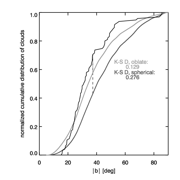
By examining the distribution in Galactic latitude of the detected clouds, we can determine whether they are linked to the Galactic disk: a distribution that is oblate in the plane of the Galaxy would indicate a relationship to the Galactic disk. The method is to construct a simplified model of the distribution of these clouds and then compare it with our observed distribution using the Kolmogorov-Smirnoff (K-S) D-statistic. The D-statistic is simply the largest difference between the cumulative distribution functions (CDFs) of the data and model. In this way we can fit a parameter in our simplified model to the data.
We choose a model that captures the relative scale distance at which these objects can be seen in the plane of the Galaxy to the scale height of a population above the disk. We call this ratio of scales . If the clouds are independent of the orientation of the Galactic plane, the K-S D-statistic should be at a minimum for a spherical distribution, . If they do follow the plane, and can be seen out past their Galactic scale height, should have a significantly smaller D-statistic. Our model simply assumes that clouds are equally detectable along the surface defined by
| (3) |
where is an arbitrary distance, and are distances from the Sun, with toward the Galactic center and pointing towards the north Galactic cap. We also assume the probability of detecting a cloud at great distance drops to zero, and that the functional form by which it drops is the same along each axis. We then compute the distribution of clouds we expect to observe from this model as a function of , given the footprint of the GALFA-HI data set, and compute the K-S D-statistic.
As shown in Fig. 16, we find that a spherical distribution is a much poorer fit to the data () than an oblate distribution (), but that we cannot distinguish between distributions with . This is because we have very little coverage in the Galactic plane, where a very oblate distribution would generate a very large number of clouds. Therefore, we see evidence that significantly more clouds are located toward the plane of the disk. This suggests an oblate cloud distribution and implies that the bulk of the clouds are related to the disk.
As mentioned in Section II, the Arecibo telescope does not allow an unbiased access to all Galactic latitudes. Currently, most of our coverage is at intermediate Galactic latitudes, . We will add in the future data from lower latitudes: =[-10:10] from I-GALFA (Inner-Galaxy ALFA Low-Latitude H I Survey). This will allow us to constrain better the latitude modeling and/or any potential variation in the cloud properties with Galactic latitude.
VII.2 Galactic Velocity Distribution
We extend the analysis of the previous section by examining the distribution of velocities. In theory, it is possible to use the distribution of velocities to determine whether the clouds are corotating with the disk or whether they are independent of disk rotation. This velocity distribution, interesting in its own right, can also help shed light on the typical distances to the clouds. In addition, modeling of the velocity distribution depends less on our incomplete survey coverage (Section II) and offers a wider range of data points for the comparison of various distributions.
VII.2.1 Galactic Model
In this model we generate a large number of clouds which populate (, , ) space, and have velocities related to the bulk rotation of the Galactic disk. To do this we assume the clouds populate an oblate distribution with and some variable distance scale (see Equation 3). We assume the clouds follow cylindrical Galactic rotation with a flat rotation curve at kms-1. In addition to their rotation velocity, we impart to them a variable random radial velocity, . We constrain the clouds to lie in our observational footprint and to meet the simple detection criterion that they do not lie in regions with background brightness temperature in HI above 4 K, which is consistent with our completeness test (Section III.3). We compute this background brightness using the 36′ resolution LAB survey ([30]).
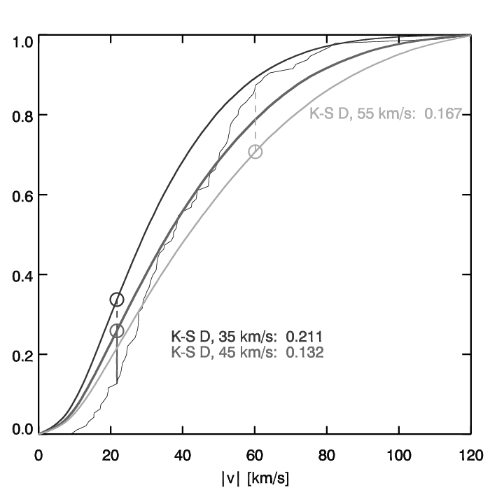
We find that comparing our model to the data does not constrain the distance to the clouds under the assumption of corotation. We can, however, fit to the random velocity component, , independent of and corotation. Using the K-S D statistic, as in Section VII.1, we find that a random radial velocity of 45 km s-1is near the best fit to the data, with a variation from this value of 10 km s-1 being noticeably worse (see Fig. 17). Assuming there is no preferential direction for this random velocity, we can multiply by to find a true 3-space random velocity of km s-1.
VII.2.2 Circumgalactic Model
We can also generate a model with the basic assumption that the clouds are beyond, but around, the Galaxy, and therefore have velocities near to zero (i.e. they are in the rest frame of the Milky Way’s barycenter). As in the Galactic model, we include the selection effects of our data set when producing the model. We include a of 45 kms-1 as in the Galactic model. We find that the circumgalactic model is qualitatively a very poor fit to the data (see Figure 18) – many observed clouds lie in areas where the model predicts almost no clouds (e.g. 30 km s-1, 90 degrees), and the model predicts many clouds where none are observed (e.g. km s-1, km s-1). We note that by increasing we could modify the model to predict more clouds in areas where there are discrepancies, but this would have the effect of also producing more model clouds out to extreme velocities, where clouds are not observed. Based on this model we conclude that the observed clouds must be related to the Galactic disk. This conclusion is consistent with, but entirely independent of, our conclusion in Section VII.1.
VIII Distance constraints: other methods
The distances to some of the cataloged clouds in the Ist and IVth Galactic quadrant can be measured using the tangent-point method. The LSR velocity at tangent points (), positions where the line of sight is perpendicular to a circle of constant Galactocentric radius, was measured from 12CO observations by Clemens (1985). We find that 17 clouds in the Ist Galactic quadrant have km s-1. If we assume that all these clouds are at the tangent point but their velocities have been perturbed from by random motions [55, 14], we can then estimate the clouds tangent point distance: d (with R kpc being the Galactocentric radius of the solar circle). Under the further assumption that Galactic rotation is constant with distance from the plane, we find that dt ranges from 0.4 to 3 kpc, with a median distance being 2.2 kpc. This would result in a median height from the Galactic Plane h1 kpc.
Another distance constraint comes from the method applied by Stanimirovic et al. (2006). Compact clouds are cold with properties similar to what is found for typical Galactic CNM clouds, or they show evidence for the existence of cold cores surrounded by warm envelopes. To explain the coexistence of the CNM and WNM, heating and cooling conditions need to be considered locally (Wolfire et al. 2003), and a well-defined range of thermal pressures is needed. For example, at kpc, and K cm-3. We can compare this pressure requirement with our pressure histogram in Figure 14. For a thermal pressure typical for the solar neighborhood of 3000 K cm-3, a distance of pc is required. Wolfire at al. (2003) showed that the lowest thermal pressure allowed for the CNM and WNM to coexist is K cm-3. This would place an upper limit on the cloud distance of kpc. This is in agreement with the tangent point method and suggests a possible distance range of 0.1 to 3 kpc.
The cloud distribution in Figure 5, roughly symmetric with a similar number of clouds having either negative or positive , places another constraint on the cloud distance. As most clouds in the sample have degrees, a cloud distance kpc would imply a height above the Galactic plane that is kpc. At such heights, Galactic rotation is lower than in the midplane of the Galaxy [36, 29, 34, 7]. This results in the distribution for the whole sample to be skewed towards negative velocities. This effect of a lag in clouds rotation velocity at high resulting in the LSR distribution getting skewed towards negative LSR velocities have been noted for the HVCs distribution [48] and the Milky halo stars [52]. As we do not observe this effect when considering the whole sample of compact clouds suggests that a majority of clouds are likely to be at a distance kpc.

IX Discussion
| Parameters | GALFA-HI | GASS | VGPS | Lockman clouds | VLA/WSRT |
|---|---|---|---|---|---|
| (This work) | [14] | [55] | [35] | [5] | |
| N | 0.5 | 1.4 | 18.0 | 2.0 | 0.9 |
| T (K) | 0.75 | 0.6 | 12.3 | 1.0 | 1.6 |
| V (kms-1) | 4.2 | 12.8 | 5.6 | 12.2 | 4.1 |
| Size (arcmin) | 5.0 | 29.0 | 3.4 | 22.3 | 2.3 |
Based on the modeling of spatial and velocity distributions of the whole compact cloud population, we have shown that the bulk of the compact clouds are related to the Galactic disk. The tangent point method and the consideration of the conditions required for the CNM/WNM coexistence in the ISM suggest that cloud distances are likely to be in the range of 0.1 to a few kpc. However, this still does not exclude the possibility for a few clouds to be located at very large distances. As possible scenarios for the cloud origin depend on distance, we discuss several possibilities in the following sub-sections.
IX.1 Galactic compact clouds at sub-pc scales
For a distance kpc, with a typical size of pc, we are dealing with nearby Galactic clouds. In this case, a significant fraction of clouds would have 1 cm-3 and a total pressure 1000 K cm-3. The cloud HI mass (shown in Figure 15, left) would be M⊙. However, at a distance as low as 100 pc these properties become slightly more extreme: 10 cm-3, 3000 K cm-3, M⊙, and clouds would have a linear size of AU. At this distance and assuming a velocity gradient of 2 km s-1 arcmin-1, the length doubling timescale for clouds/filaments would be very short, yr. Such short lifetimes suggest transient and recently produced objects.
In any case, the properties (size, temperature, HI column density, HI mass) of such sub-pc clouds may be similar to those of the low-column density absorbers [6, 57]. This possible connection is also supported by the WSRT HI emission observations by Braun & Kanekar (2005), who found several compact clouds in the proximity of one of the low column density absorbers seen in HI absorption. In this scenario, the compact clouds may represent large and low column-density examples of the population of CNM clouds on sub-pc scales. The most extreme CNM clouds, so called “tiny scale atomic structure” (TSAS), reach scales of a few AU, appear over-dense and over-pressured relative to the traditional CNM, and were once postulated to comprise up to 15% of the CNM (Frail et al. 1994; Heiles 1997). The obvious questions are, how do such small and isolated clouds form and survive in the ISM, and what role do they play within the general ISM?
One possible scenario that can explain the formation and maintenance of compact cold clouds in the ISM is interstellar turbulence. Recently numerical simulations of the ISM have started to describe cold and warm atomic gas with a numerical resolution and dynamic range approaching realistic physical scales e.g. Vazquez-Semadeni et al. [61], de Avillez & Breitschwerdt [12], Audit & Hennebelle [1]. The numerical simulations by Audit & Hennebelle (2005) show that a collision of incoming turbulent flows can initiate condensation of the WNM into cold neutral clouds. A collision of incoming WNM streams creates a thermally unstable region of higher density and pressure but lower temperature, which further fragments into small cool structures. The abundance of cold structures, as well as their properties, depends heavily on the properties of the underlying turbulent flows. For example, Audit & Hennebelle (2005) find that a significant fraction of the CNM structures formed in the case of very turbulent flows have thermal pressures of K cm-3, temperatures 100 K and volume density n cm-3. These CNM structures are thermally stable, long lived ( Myr) and in the case of stronger turbulence they are more rounded, similar to the compact clouds in our sample.
In a similar approach, Koyama & Inutsuka (2002) showed that a thermally unstable shock-compressed layer, formed from the WNM compression by supernova explosions, can also fragment into small, cold, turbulent condensations as a result of the thermal instability. As the ISM is frequently compressed by supernova explosions, fragmentation of the shock-compressed medium can also be a potential mechanism for the formation of compact clouds.
Another possibility may be provided by stellar outflows. HI emission has been detected in the circumstellar shells of a variety of evolved stars, viz. asymptotic giant branch stars, oxygen-rich and carbon-rich stars, semi-regular and Mira variables, and planetary nebulae [18]. For example, Matthews et al. (2008) found an extended tail of HI associated with the AGB star Mira and argued that HI tails are likely to be a common feature of evolved stars undergoing mass loss. Furthermore, HI has also been detected in emission/absorption toward several planetary nebulae (Gussie & Taylor 1995, Rodriguez et al. 2002). Our cross-correlation of the compact cloud catalog with the catalogue of variable stars by Downes et al. (2006) suggests that a subset of clouds has at least one variable star within a radius of 1 degree.
The association of HI clouds with variable stars at angular distances of degrees has been noticed before. Matthews et al. (2008) found HI emission as far as away from a Mira variable. Gerard & Le Bertre (2006) also reported evidence that HI emission associated with circumstellar envelopes may be offset from the position of the central star. Assuming that the detected HI clouds are the circumstellar HI associated with variable stars, for a typical distance of 100 pc and an expansion velocity of 5 km s-1 seen for circumstellar HI [18], a degree separation of the HI clouds from the variable star corresponds to an HI mass of M⊙, an HI diameter of 1.7 pc, and a characteristic time-scale of 0.34 Myr. All three parameters agree well with the ones found in the HI survey of circumstellar envelopes around evolved stars [18]. Hence it is likely that some of the compact HI clouds could be related to the outflows from these stars.
Once formed by turbulence and/or stellar outflows and injected into the surrounding medium, these isolated compact clouds of cold, low column density HI will be immersed in the warm/hot ambient gas. The obvious question that arises is how are such compact clouds able to survive without being quickly evaporated. From Eq. (47) in McKee & Cowie [39], the mass-loss of a compact HI cloud embedded in a hot plasma ( K) is M⊙ Myr-1, whereas if the clouds are embedded in large warm envelopes ( K), the evaporation mass-loss is ten times smaller. This would imply that the compact clouds may be evaporating on a timescale of Myr, due to a combination of conductive heat transfer and/or Kelvin-Helmholtz instabilities from the surrounding warm/hot medium [57, 9].
IX.2 Compact clouds in the disk-halo interface region
If at a distance of a few kpc, the majority of compact clouds would have 100 K cm-3, 1.0 cm-3, a height of a few kpc above the disk, and a corresponding HI mass of M⊙. In this scenario, observed cloud properties are similar to numerous HI clouds found in the Galactic disk-halo interface region.
Recent HI observations have shown that the disk-halo interface of our Galaxy is not smooth, but populated with discrete HI clouds. Observations with the Green Bank telescope (GBT) found discrete HI clouds in the halo of the inner Galaxy (Lockman 2002). Although these clouds, often referred to as “Lockman’s clouds”, are located 900 pc below the plane, they appear to be dynamically related to the disk. Further, [55] discovered many clouds at forbidden velocities in the inner Galaxy using data from the VLA Galactic Plane Survey (VGPS). Despite their forbidden velocities, those clouds follow the Galactic emission. Similarly, Ford et al. (2008) detected over 400 HI clouds in the lower halo of the inner Galaxy using the Galactic All-Sky Survey (GASS), with properties similar to the clouds discovered by Lockman (2002). [58], using the GALFA-HI precursor observations, found numerous clouds in the disk-halo interface of the outer Galaxy, indicating that this phenomenon is not restricted to the inner Galaxy. Finally, using the interferometric data from the Westerbork Synthesis Radio Telescope (WSRT) and the Very Large Array (VLA), [5] studied the HI emission at low, intermediate and high radial velocities along four random lines of sight toward quasars which had previous detections of weak CaII and NaI absorption features. They found several compact and cold clumps of neutral gas at velocities similar to those of the optical absorption.
Table 3 shows a comparison of the compact clouds from this work with the clouds discovered in the recent Galactic surveys. Based on their physical parameters, NHI, T and V, compact clouds from the GALFA-HI survey are the most similar to the low-column density HI clumps seen in the HI interferometric observations along the sight-lines of CaII and NaI absorbers (Bekhti et al. 2009). However, most differences between various studies stem from the difference in angular resolution and sensitivity of various surveys. For example, higher values of NHI and T for the [5] clouds compared to our sample are mainly due to the difference in angular resolution of the Arecibo (3.5 arcmin) and WSRT/VLA observations (1.6 arcmin). Larger size and velocity line-width of the GASS and GBT clouds samples are largely caused by large telescope beams (15 arcmin and 9 arcmin for the Parkes telescope and the GBT, respectively) and the blending of smaller clouds. The HI clouds in the disk-halo interface region are generally thought to originate from the condensation of hot gas expelled from the disk by superbubbles [28]. Hence, these compact clouds in the disk-halo interface could play an important role in studying the mass circulation between the Milky Way disk and the halo.
An alternative mechanism that may be able to explain the existence of compact clouds in the disk-halo interface region was recently proposed by Heitsch & Putman (2009), and involves re-cooling of inflowing gas. Simulations show that as warm/ionized clouds approach the Galactic disk, they encounter denser and denser material, which leads to the compression of clouds and causes them to slow down and recool, forming intermediate and low-velocity clouds close to the Galactic disk. The compact clouds in our sample may be able to fit into this framework, thus representing a later stage of the infall process for HVCs. The observed compact clouds may be getting integrated and digested by the disk, and hence provide a smooth buildup of fresh star formation fuel for the Galactic disk. The random radial velocity component of 45 km s-1 for the clouds found in Section 7.2.1, corresponds to T K, and may be interpreted as compact clouds being condensed out of an extended warm/hot layer in the disk-halo interface as traced by O VI absorption lines [53]. Future metallicity and dust-to-gas ratio observations of compact clouds would be the crucial test of the cloud infall hypothesis.
IX.3 Compact clouds at extreme distances
As discussed in Section V, if the compact clouds are self-gravitating systems, they have to be extremely dark matter dominated in order to be stable, having more than 99% of the total mass as dark. The presence of a large number of such low mass, dark matter halos have been predicted by cosmological CDM simulations (Klypin et al. 1999, Moore et al. 1999). [54] showed that most of the gas in low mass halos should be found in a thermally stable, ionized/WNM phase, within which cold cores may be able to form. However, such models require the clouds to be at large distances (100 kpc). We note that although the compact cloud sample as a whole cannot be circumgalactic, from our statistical analysis in Section VII.2, we cannot rule out the possibility that some of the clouds could be at large distance, and hence they could be associated with the dark matter mini halos in the vicinity of the Milky Way, as predicted by cosmological CDM simulations. Recently, Giovanelli et al.(2010) found a set of isolated, HI sources in the ALFALFA survey and argued that these could be associated with isolated mini-halos in the outskirts of the Local Group. Again, metallicity and dust-to-gas ratio observations of these clouds should be able to address the mini-halo possibility.
X Summary and Conclusions
The Galactic Arecibo L-band Feed Array HI (GALFA-HI) survey is successfully mapping the entire Arecibo sky at 21-cm. The survey covers a velocity range of 700 to 700 kms-1 (LSR) at a velocity resolution of 0.18 kms-1 and an angular resolution of 3.5 arcmin. The unprecedented resolution and sensitivity of the GALFA-HI survey resulted in the detection of numerous isolated, compact HI clouds at low Galactic velocities, which are distinctly separated from the disk HI emission. In the limited area of 4600 deg2 surveyed so far, we have detected 96 such compact clouds. The detected clouds are cold with median T K. Moreover, these clouds are quite compact and faint with median properties of 5 arcmin in angular size, 0.75 K in peak brightness temperature, and NHI of cm-2. Most of the clouds deviate from Galactic rotation at the 20-30 kms-1 level, and a significant fraction shows evidence for a multiphase medium and/or velocity gradients. No counterparts for these clouds were found in other wavebands.
From the modeling of spatial and velocity distribution of the whole compact cloud population, we find that the bulk of the population is related to the Galactic disk and their distances are likely to be in the range of 0.1 to a few kpc. This is consistent with distance estimates based on the thermal pressure requirements for the CNM and the WNM coexistence, and the tangent point method for a subset of clouds.
If the clouds are at a distance 1 kpc, they would represent low-column density examples of the population of CNM Galactic clouds on sub-pc scales. Possible mechanisms for the formation of such clouds involve stellar outflows, and/or condensation of the WNM by the collision of turbulent flows. Once formed, such cold, low column density, compact HI clouds would evaporate on timescales of Myr due to the combination of conductive heat transfer and/or Kelvin-Helmholtz instabilities from the surrounding warm/hot medium. Conversely, if the clouds are at distances of a few kpc, they are similar to the HI clumps observed in the Galactic disk-halo interface region. One potential mechanism that may be able to explain the existence of such cold clouds was recently proposed by [25] and involves the re-cooling of inflowing gas. Finally, our modeling of cloud distributions cannot exclude the possibility of sporadic compact clouds being at large distances. If being at large distances and self-gravitating, such clouds would be extremely dark matter dominated and may be related to the dark matter mini-halos predicted by cosmological simulations.
Our completeness check of the compact cloud catalog, showed that we are most likely missing about one quarter of the clouds due to our selection biases for regions where Galactic background is below 4 K. In addition, we cannot detect any clouds in regions where the Galactic background exceeds 4 K. We speculate that faint, compact HI clouds are probably widespread throughout the Galaxy, but we are able to detect them only in the regions with low Galactic emission. In the future, by completing the GALFA-HI survey and applying automated methods for cloud detection we will collate a larger sample of compact clouds and extend our latitude coverage to degrees. This will allow us to better constrain cloud spatial distribution through the latitude and velocity modeling discussed in the paper. In addition, we will investigate whether compact clouds are related to local events, such as stellar winds or large-scale atomic flows, or are globally distributed across the disk with notable kinematic properties. To fully study this cloud population we will have to wait for the next generation radio telescopes (Australian SKA Pathfinder, MeerKAT, or the Square Kilometer Array) which will play an important role in providing a census of compact clouds by providing sensitive and high-resolution surveys, capable of filtering large-scale diffuse HI emission.
References
- [1] Audit, E. & Hennebelle, P. 2005, A&A, 433, 1
- [2] Auld et al. 2006, MNRAS, 371, 1617
- [3] Begum, A., Chengalur, J . N., Karachentsev, I. D., Sharina, M. E. & Kaisin, S. S., 2008, MNRAS, 386, 1667
- [4] Begum, A., Chengalur, J . N., Karachentsev, I. D., Kaisin, S. S. & Sharina, M. E., 2006, MNRAS, 365, 1220
- [5] Bekhti, B. N., Richter, P., Winkel, B., Kenn, F. & Westmeier, T. 2009, A&A, 503, 483
- [6] Braun, R. & Kanekar, N. 2005, A&A, 436, 53L
- [7] Collins, J. A., Benjamin, R. A. & Rand, R. J., 2002, ApJ, 578, 98
- [8] Clemens, D. P., 1985, ApJ, 295, 422
- [9] Dedes, L., & Kalberla, P. W. M., 2010, A&A, 509, A60
- [10] Dedes, L., Dedes, C. & Kalberla, P. W. M., 2008, A&A, 491, L45
- [11] Downes, R. A., Webblink, R. F., Shara, M. M., Ritter, H., Kolb, U. & Duerbeck, H. W., 2006, VizieR On-line Data Catalog: V/123A
- [12] de Avillez, M. A. & Breitscwerdt, D. 2005, ApJ, 634, L65
- [13] Field, G. B., Goldsmith, D. W., & Habing, H. J. 1969, ApJ, 155, L149
- [14] Ford, A. H., McClure-Griffiths N. M, Lockman, F. J., Bailin, J., Calabretta, M. R., Kalberla, P. M. W., Murpht, T. & Pisano D. J. 2008 ApJ, 688, 290
- [15] Frail, D. A., Weisberg, J. M., Cordes, J. M., & Mathers, C. 1994, ApJ, 436, 144
- [16] Frisch, P. C., Grodnicki, L.,& Welty, D. E. 2002, ApJ, 574, 834
- [17] Guram, S. S., & Taylor, A. R., 2009, ASPC, 407, 282
- [18] Gerard, E., & Le Bertre, T., 2006, AJ, 132, 2566
- [19] Gibson, S. J., Taylor, R., Higgs L. A., Brunt, C. M. & Dewdney, P. E., 2005, ApJ, 626, 195
- [20] Giovanelli, R., Haynes, M. P., Kent, B. R. & Adams, E. A. K., 2010, ApJ, 708, 22L
- [21] Giovanelli, R., et al. 2005, AJ, 130, 2598
- [22] Gooch, R., 1996, ASPC, 101, 80
- [23] Gussie, G. T. & Taylor, A. R., 1995, MNRAS, 273, 801
- [24] Heiles, C. 1997, ApJ, 481, 193
- [25] Heitsch, F. & Putman, M. E. 2009, ApJ, 698, 1485
- [26] Heiles, C. & Troland, T. H. 2003a, ApJS, 145, 329
- [27] Heiles, C. & Troland T. H., 2003b, ApJ, 586, 1067
- [28] Houck, J. C. & Bregman, J. N., 1990, ApJ, 352, 506
- [29] Kalberla, P. M. W. & Kerp, J., 2009, ARA&A, 47, 27
- [30] Kalberla, P. M. W., Burton, W. B., Hartmann, D., Arnal, E. M.,Bajaja, E., Morras, R. & Poppel, W. G. L., 2005, A&A, 440, 775
- [31] Kalberla, P. M. W. & Haud, U., 2006, A&A, 455, 481
- [32] Klypin, A., Kravtsov, A., Valenzuela, O. & Prada F. 1999 ApJ, 522, 82
- [33] Koyama, H. & Inutsuka, S. 2002, ApJ, 564, L97
- [34] Levine, E. S., Heiles, C. & Blitz, L., 2008, ApJ, 679, 1288
- [35] Lockman, F. J., 2002 ApJ, 580, L47
- [36] Marinacci, F., Fraternalli, F., Ciotti, L. & Nipoti, C., 2010, MNRAS, 401, 2451
- [37] Matthews, L. D., Libert, Y., Gerard, E., Le Berte, T. & Reid, M. J., 2008, ApJ, 684, 603
- [38] McClure-Griffiths, N. M., Pisano, D. J., Calabretta, M. R., Ford, H. Alyson, Lockman, Felix J., Staveley-Smith, L., Kalberla, P. M. W., Bailin, J., Dedes, L., Janowiecki, S., Gibson, B. K., Murphy, T., Nakanishi, H. & Newton-McGee, K.,2009, ApJS, 181, 398
- [39] McKee, C. F. & Cowie, L. L. 1977, ApJ, 215, 213
- [40] McKee, C. F. & Ostriker, J. P. 1977, ApJ, 218, 148
- [41] Moore, B., Ghigna, S., Governato, F., Lake, G., Quinn, T.,Stadel, J. & Tozzi P. 1999 ApJ, 524, L19
- [42] Muller, H., Frisch, O. C., Florinski, V. & Zank, G. P., 2006, ApJ, 647, 1491
- [43] Philips, J. P., 1999, A&AS, 134, 241
- [44] Putman, M. E., et al. 2002, AJ, 123, 873
- [45] Redfield, S., & Linsky, J. L. 2008, ApJ, 673, 283
- [46] Redfield, S., & Linsky, J. L. 2002, ApJS, 139, 439
- [47] Rodriguez, L. F., Goss, M. W., & Williams, R. 2002, ApJ, 574, 179
- [48] Peek, J. E. G., Heiles, C., Putman, M. E. & Douglas, K., 2009, ApJ, 692, 827
- [49] Peek, J. E. G. & Heiles, C., 2008, arXiv:0810.1283
- [50] Rosolowsky, E., Engargiola, G., Plambeck, R. & Blitz, L., 2003, ApJ, 599, 258
- [51] Ryan-Weber, E. V., Begum, A., Oosterloo, T., Pal, S., Irwin, M. J., Belokurov, V., Evans, N. W. & Zucker, D. B., 2008, MNRAS, 384, 535
- [52] Schneider, P., Extragalactic Astronomy and Cosmology: An Introduction, Springer-Verlag Berlin Heidelberg 2006
- [53] Savage, B. D., Sembach, K. R., Wakker, BP B., Richter, P., Meade, M., Jenkins, E. B., Shull, J. M., Moos, H. W. & Sonneborn, G., 2003, ApJS, 146, 125
- [54] Sternberg, A., McKee, C. F. & Wolfire, M. G., 2002, ApJS, 143, 419
- [55] Stil, J. M., Lockman, F. J., Taylor, A. R., Dickey, J. M., Kavars, D. W., Martin, P. G., Rothwell, T. A., Boothroyd, A. I. & McClure-Griffiths N. M. 2006 ApJ, 637, 366
- [56] Stil, J. M., Taylor, A. R., Dickey, J. M., Kavars, D. W., Martin, P. G., Rothwell, T. A., Boothroyd, A. I., Lockman, F. J. & McClure-Griffiths N. M. 2006 ApJ, 132, 1158
- [57] Stanimirović, S., & Heiles, C., 2005, ApJ, 631, 371
- [58] Stanimirović, S., et al., 2006, ApJ, 653, 1210
- [59] Stanimirović, S., Heiles, C. & Kanekar, N., 2007, ASPC, 365, 22
- [60] Stanimirović, S., Hoffman, S., Helies, C., Douglas, K. A., Putman, M. & Peek, J. E. G. 2008, ApJ, 680, 276
- [61] Vazquez-Semadeni, E., Ryu, D., Passot, T., Gonzalez, R. & Gazol, A., 2006, ApJ, 643, 245
- [62] Wakker, B. P., 2004, High Velocity Clouds (ASSL, Vol. 312), ed. H. van Woerden, B. P. Wakker, U. J. Schwarz, & K. S. de Boer (Dordrecht: Kluwer), 25
- [63] Wakker, B. P., 2001, ApJS, 136, 463
- [64] Wakker, B. P., 1991, A&A, 250, 499
- [65] Wood, B. E., Redfield, S., Linsky, J. L., Müller, H. R., & Zank, G. P. 2005, ApJS, 159, 118
- [66] Welsh, B. Y., Lallement, R., Vergely, J. L. & Raimond, S., 2010, A&A, 510, 54
- [67] Wolfire, M. G., McKee, C. F., Hollenbach, D., & Tielens, A. G. G. M. 2003, ApJ, 587, 278