MONOPOLE-ANTIMONOPOLE PAIR DYONS

In order to solve the for the MAP dyons solutions, the ansatz (10) is substituted into the equations of motion (4) and the 15 equations of motion are reduced to eight coupled second order partial differential equations. These eight equations are solved asymptotically first at small and then at large distances. In these asymptotic regions, the time component of the gauge field and the Higgs field are parallel in the isospin space, that is $\Phi_{1}={\cal A}_{1}$ and $\Phi_{2}={\cal A}_{2}$. The asymptotic solutions and boundary conditions at small distances that will give rise to finite energy MAP dyons solutions are

	$\displaystyle\psi_{A}(0,\theta)=R_{A}(0,\theta)=0,~~~A$	$\displaystyle=$	$\displaystyle 1,2;$
	$\displaystyle\sin\theta~\Phi_{1}(0,\theta)+\cos\theta~\Phi_{2}(0,\theta)$	$\displaystyle=$	$\displaystyle 0$
	$\displaystyle\sin\theta~{\cal A}_{1}(0,\theta)+\cos\theta~{\cal A}_{2}(0,\theta)$	$\displaystyle=$	$\displaystyle 0$
	$\displaystyle\left.\frac{\partial}{\partial r}\left(\cos\theta~\Phi_{1}(r,\theta)-\sin\theta~\Phi_{2}(r,\theta)\right)\right|_{r=0}$	$\displaystyle=$	$\displaystyle 0$
	$\displaystyle\left.\frac{\partial}{\partial r}\left(\cos\theta~{\cal A}_{1}(r,\theta)-\sin\theta~{\cal A}_{2}(r,\theta)\right)\right|_{r=0}$	$\displaystyle=$	$\displaystyle 0.$		(13)

At large distances, the asymptotic solution can be written as

	$\displaystyle\psi_{1}(\infty,\theta)=2,~~\psi_{2}(\infty,\theta)=2n,~~~R_{A}(\infty,\theta)$	$\displaystyle=$	$\displaystyle 0,$
	$\displaystyle\Phi_{1}(\infty,\theta)=\xi\cos\theta,~~~\Phi_{2}(\infty,\theta)$	$\displaystyle=$	$\displaystyle\xi\sin\theta,$
	$\displaystyle{\cal A}_{1}(\infty,\theta)=\eta\xi\cos\theta,~~~{\cal A}_{2}(\infty,\theta)$	$\displaystyle=$	$\displaystyle\eta\xi\sin\theta$		(14)
	$\displaystyle R_{A}(r,\theta)|_{\theta\rightarrow 0,~\pi}=\Phi_{2}(r,\theta)|_{\theta\rightarrow 0,~\pi}={\cal A}_{2}(r,\theta)|_{\theta\rightarrow 0,~\pi}$	$\displaystyle=$	$\displaystyle 0,$
	$\displaystyle\partial_{\theta}\psi_{A}(r,\theta)|_{\theta\rightarrow 0,~\pi}=\partial_{\theta}\Phi_{1}(r,\theta)|_{\theta\rightarrow 0,~\pi}=\partial_{\theta}{\cal A}_{1}(r,\theta)|_{\theta\rightarrow 0,~\pi}$	$\displaystyle=$	$\displaystyle 0,$		(15)

where $A=1,2$, and the expectation value $\xi=\frac{\mu}{\sqrt{\lambda}}=1$. The numerical MAP dyons solutions connecting the asymptotic solutions (13) to (14) and subjected to the boundary conditions (15) together with the gauge fixing condition [8]

$$\partial_{r}R_{1}-r\partial_{\theta}\psi_{1}=0,$$

(16)

were solved using the Maple 12 and MatLab R2009a softwares. The second order equations of motion (4) which are reduced to eight partial differential equations with the ansatz (10) are then transformed into a system of nonlinear equations using the finite difference approximation. This system of nonlinear equations are then discretized on a non-equidistant grid of size $70\times 60$ covering the integration regions $0\leq\bar{x}\leq 1$ and $0\leq\theta\leq\pi$. Here $\bar{x}$ is the finite interval compactified coordinate given by $\bar{x}=\frac{r}{r+1}$. The partial derivative with respect to the radial coordinate is then replaced accordingly by  $\partial_{r}\rightarrow(1-\bar{x})^{2}\partial_{\bar{x}}$  and  $\frac{\partial^{2}}{\partial r^{2}}\rightarrow(1-\bar{x})^{4}\frac{\partial^{2}}{\partial\bar{x}^{2}}-2(1-\bar{x})^{3}\frac{\partial}{\partial\bar{x}}$ . First of all, we used Maple to find the Jacobian sparsity pattern for the system of nonlinear equations. After that we provide this information to Matlab to run the numerical computation. The system of nonlinear equations are then solved numerically using the trust-region-reflective algorithm by providing the solver with good initial guess.

The second order equations of motion Eq. (4) were solved when the $\phi$-winding number $n=1,2$ and with zero Higgs potential, that is $\lambda=\mu=0$ but with nonzero expectation value $\xi=1$ and finally with $\lambda=\mu=1$ and expectation value $\xi=1$.

In the Prasad-Sommerfield limit where $\lambda=0$, the ansatz (10) can be simplified by letting

$\displaystyle{\cal A}_{1}(r,\theta)=\eta\Phi_{1}(r,\theta)~~\mbox{and}~~{\cal A}_{2}(r,\theta)=\eta\Phi_{2}(r,\theta)$

(17)

hence making the gauge potential $A_{0}^{a}$ parallel to the Higgs field $\Phi^{a}$ in isospin space.

Upon substituting ansatz (10) and (17) into the equations of motion (4), the resulting equations of motion are simplified to,

$\displaystyle D^{i}F^{a}_{ij}=\partial^{i}F^{a}_{ij}+\epsilon^{abc}A^{bi}F^{c}_{ij}=\epsilon^{abc}\tilde{\Phi}^{b}D_{j}\tilde{\Phi}^{c},~~~D^{i}D_{i}\tilde{\Phi}^{a}=0,$

(18)

where $\tilde{\Phi}^{a}=\sqrt{1-\eta^{2}}~\Phi^{a}=\mbox{sech}\gamma~\Phi^{a}$, the covariant time derivative $D_{0}\Phi^{a}=0$, and the electric field $E^{a}_{i}=F^{a}_{i0}=-\eta D_{i}\Phi^{a}$. The time component of the ’t Hooft gauge potential becomes, $A_{0}=\eta|\Phi|$. Hence the ’t Hooft electric field is non zero when $\eta\not=0$ and the monopole becomes a dyon.

The ’t Hooft magnetic field $B_{i}$ is made up of two parts, the gauge part and the Higgs part,

	$\displaystyle B_{i}$	$\displaystyle=$	$\displaystyle B^{G}_{i}+B^{H}_{i},$
	$\displaystyle B^{G}_{i}$	$\displaystyle=$	$\displaystyle-\epsilon_{ijk}\partial_{j}A_{k}~~~\mbox{and}~~~B^{H}_{i}=\frac{1}{2}\epsilon_{ijk}\epsilon^{abc}\hat{\Phi}^{a}\partial_{j}\hat{\Phi}^{b}\partial_{k}\hat{\Phi}^{c}.$		(19)

With some calculations, the gauge part of the magnetic field is given by

	$\displaystyle B^{G}_{i}$	$\displaystyle=$	$\displaystyle-n\epsilon_{ijk}\partial_{j}\sin\kappa~\partial_{k}\phi,~~$
	$\displaystyle\mbox{where},~~\sin\kappa$	$\displaystyle=$	$\displaystyle\frac{\sin\theta}{n}\left(\psi_{2}\frac{\Phi_{2}}{|\Phi|}-R_{2}\frac{\Phi_{1}}{|\Phi|}\right),$		(20)

To calculate for the ’t Hooft magnetic field $B_{i}^{H}$, we rewrite the Higgs field from the spherical to the Cartesian coordinate system,

	$\displaystyle\Phi^{a}$	$\displaystyle=$	$\displaystyle\Phi_{1}~\hat{n}^{a}_{r}+\Phi_{2}~\hat{n}^{a}_{\theta}+\Phi_{3}~\hat{n}^{a}_{\phi}$		(21)
		$\displaystyle=$	$\displaystyle\tilde{\Phi}_{1}~\delta^{a1}+\tilde{\Phi}_{2}~\delta^{a2}+\tilde{\Phi}_{3}~\delta^{a3},$

	$\displaystyle\mbox{where}~~~\tilde{\Phi}_{1}$	$\displaystyle=$	$\displaystyle\sin\theta\cos n\phi~\Phi_{1}+\cos\theta\cos n\phi~\Phi_{2}-\sin n\phi~\Phi_{3}=|\Phi|\cos\alpha\sin\beta$
	$\displaystyle\tilde{\Phi}_{2}$	$\displaystyle=$	$\displaystyle\sin\theta\sin n\phi~\Phi_{1}+\cos\theta\sin n\phi~\Phi_{2}+\cos n\phi~\Phi_{3}=|\Phi|\cos\alpha\cos\beta$
	$\displaystyle\tilde{\Phi}_{3}$	$\displaystyle=$	$\displaystyle\cos\theta~\Phi_{1}-\sin\theta~\Phi_{2}=|\Phi|\sin\alpha.$		(22)

The Higgs unit vector can be simplified to

	$\displaystyle\hat{\Phi}^{a}$	$\displaystyle=$	$\displaystyle\cos\alpha\sin\beta~\delta^{a1}+\cos\alpha\cos\beta~\delta^{a2}+\sin\alpha~\delta^{a3},$
	$\displaystyle\sin\alpha$	$\displaystyle=$	$\displaystyle\frac{\Phi_{1}}{|\Phi|}\cos\theta-\frac{\Phi_{2}}{|\Phi|}\sin\theta,~~~\beta=\frac{\pi}{2}-n\phi,$		(23)

and the ’t Hooft magnetic field is reduced to only the $\hat{r}_{i}$ and $\hat{\theta}_{i}$ components,

	$\displaystyle B_{i}^{H}$	$\displaystyle=$	$\displaystyle-n\epsilon_{ijk}\partial^{j}\sin\alpha\partial^{k}\phi$		(24)
		$\displaystyle=$	$\displaystyle-\frac{n}{r^{2}\sin\theta}\left\{\frac{\partial\sin\alpha}{\partial\theta}\right\}\hat{r}_{i}+\frac{n}{r\sin\theta}\left\{\frac{\partial\sin\alpha}{\partial r}\right\}\hat{\theta}_{i}.$

From our numerical calulation, we managed to plot magnetic field lines of the MAP dyons when $n=1$ for values of $\lambda=0,1$ and $\eta=0.20,0.90,0.98$ as in Figure 1 and when $n=2$ for values of $\lambda=0,1$ and $\eta=0.20,0.90,0.98$ as in Figure 2.

From Eq.(8), the net magnetic charges enclosed by the upper and lower hemi-sphere at infinity are calculated to be,

	$\displaystyle M_{+}$	$\displaystyle=$	$\displaystyle-\left.\frac{n}{2}\sin\alpha\right|^{\frac{\pi}{2}}_{0,r\rightarrow\infty}=+n,$
	$\displaystyle M_{-}$	$\displaystyle=$	$\displaystyle-\left.\frac{n}{2}\sin\alpha\right|^{\pi}_{\frac{\pi}{2},r\rightarrow\infty}=-n,~~n=1,2,$		(25)

respectively. Hence the magnetic charge in the upper and lower hemi-sphere is $+n$ and $-n$ respectively and the net magnetic charge of the MAP dyon is zero. For the MAP dyon to exist, $n=1,2$ and when $n=3$, the MAP dyon cease to exist and a vortex ring dyon is formed instead [8]. Following ’t Hooft’s definition for the electromagnetic field, Eq. (6), the magnetic charges of $n=\pm 1,\pm 2$, are all located at the zeros of the Higgs field and the MAP separations $d(n,\lambda,\eta)$ for different values of $n$, $\lambda$, and $\eta$ are as given in Table 1 and 2.

From Figure 1 and Figure 2, we can generally conclude that when $\lambda=1$, the MAP separations are smaller than when $\lambda=0$ for given values of $\eta$ and $n$ as the interaction between Higgs field is attractive. When $n=2$, the MAP separations are smaller than when $n=1$ for fixed values of $\lambda$ and $\eta$ as the MAP possess unlike magnetic charges that attract. When the value of $\eta$ increases the electric charges also increases and for fixed values of $\lambda$ and $n$, the MAP separations get wider as the MAP possess similiar electric charges that repel. Hence the MAP separation $d(n,\lambda,\eta)$ varies with $n$, $\lambda$, and $\eta$. From our numerical calculations, we found that when $\lambda=0$, $d(n,0,\eta)$ increases with $\eta$ from $d(1,0,0)=4.20$ and $d(2,0,0)=1.79$ to infinity exponentially fast as $\eta$ approaches one. However when $\lambda=1$, $d(n,1,\eta)$ increases with $\eta$ from $d(1,1,0)=3.26$ and $d(2,1,0)=1.50$ to finite critical values of $d(1,1,1)=5.18$ and $d(2,1,1)=2.07$ respectively as $\eta$ approaches one. See Table 1 and 2.

At spatial infinity in the Higgs vacuum, the electromagnetic field can be represented uniquely by

$\displaystyle{\cal F}_{\mu\nu}$

$\displaystyle=$

$\displaystyle F_{\mu\nu}^{a}\left\{\frac{\Phi^{a}}{\xi}\right\},$

(26)

which corresponds to the unbroken U(1) symmetry. The corresponding electric and magnetic fields are then ${\cal E}_{i}={\cal F}_{i0}$ and ${\cal B}_{i}=-\frac{1}{2}\epsilon_{ijk}{\cal F}_{jk}$. However according to Coleman [9], there is no unique way of representing the electromagnetic field in the region of the monopole outside the Higgs vacuum. One proposal was as given by ’t Hooft as in Eq. (6) which will reduced to Eq. (26) at spatial infinity in the Higgs vacuum. The ’t Hooft’s magnetic field has the special property, $\partial^{i}B_{i}=0$ when $|\Phi|\not=0$. Hence with ’t Hooft’s definition of the electromagnetic field, the magnetic charges can only reside at the zeros of the Higgs field and the magnetic charges of the MAP dyon configurations are concentrated at two points along the $z$-axis where the Higgs field vanishes. Thus there are points singularities in ’t Hooft’s definition of Eq. (6), which makes it not possible to calculate and plot the magnetic and electric charge density distributions numerically with this definition.

The ’t Hooft electric field of the MAP dyon, $E_{i}=\partial_{i}A_{0}=\partial_{i}\left\{{\cal A}_{1}\frac{\Phi_{1}}{|\Phi|}+{\cal A}_{2}\frac{\Phi_{2}}{|\Phi|}\right\}$ corresponds to Eq. (26) in the Higgs vacuum. 2D vector plots of the electric field $E_{i}$ are given in Figure 1 when $n=1$ and Figure 2 when $n=2$, for $\eta=0.20,0.90,0.98$ and (a) $\lambda=0$, (b) $\lambda=1$. Unlike the magnetic field, the electric field varies proportionally with the constant $-1\leq\eta\leq 1$. Hence the electric field can be switched off by setting $\eta=0$. As the parameter $\eta$ increases from $-1$ to zero, the electric field points radially inwards and when $0<\eta\leq 1$, the electric field is radially outwards. Hence the electric charges of the both the monopole and antimonopole are positive (negative) when $\eta$ is positive (negative).

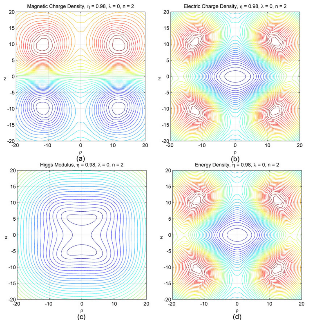
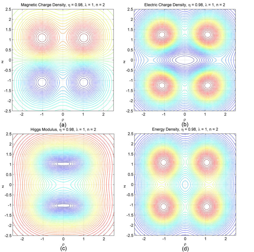
Another proposal for the electromagnetic field, ${\cal F}_{\mu\nu}=F_{\mu\nu}^{a}\left\{\frac{\Phi^{a}}{\eta}\right\}$, was given by Bogolmolny [10] and Faddeev [11]. Using this definition, Eq. (26), the magnetic charge density $g=\partial^{i}{\cal B}_{i}$ and electric charge density $q=\partial^{i}{\cal E}_{i}$ distributions can be calculated and plotted numerically as shown in Figure 3 (a), (b) to Figure 6 (a), (b) when $\lambda=0,1$ and $n=1,2$ respectively. The electric charge density, $q=\partial^{i}{\cal E}_{i}$, of the MAP dyon solutions is solely positive (negative) throughout space when $\eta$ is positive (negative). When $n=1$, the electric charge distribution of the MAP dyon is two spheres centered at the two point zeros of the Higgs field. Hence the soliton has a dumbbell shape structure.

However when $n=2$, the electric charge distribution is two horizontal toruses around the two zeros of the Higgs field as center with the $z$-axis as the symmetry axis. Contour plots of the electric charge density distribution when $n=1,2$, $\lambda=0,1$, and $\eta=0.98$ are given in Figure 3 (b) to Figure 6 (b). Contour plots of the magnetic charge density distribution, the Higgs field modulus, and energy density when $n=1,2$, $\lambda=0,1$, and $\eta=0.98$ are also given in Figure 3 (a), (c), (d) to Figure 6 (a), (c), (d) respectively.

From Gauss’ law, the total electric charge of the dyon is given by,

$\displaystyle Q(n,\lambda,\eta)=\int_{r\rightarrow\infty}{\cal E}_{i}\hat{r}_{i}~r^{2}\sin\theta~d\theta d\phi.$

(27)

The different values of $Q(n,\lambda,\eta)$ calculated for various values of $n$, $\lambda$, and $\eta$ are as tabulated in Table 1 and 2. For fixed value of $n=1,2$ and $\lambda=0$, $Q(\eta)$ increases with $\eta$ from $Q(n,0,0)=0$ and approaches infinity exponentially fast as $\eta$ approaches one. However for fixed value of $n=1,2$ and $\lambda=1$, $Q(\eta)$ increases with $\eta$ from $Q(n,1,0)=0$ to a maximum critical value of $Q(1,1,\eta)=17.61$ and $Q(2,1,\eta)=21.15$ as $\eta$ approaches one. The four parametric graphs for MAP separation $d(n,\lambda,\eta)$ versus total electric charge $Q(n,\lambda,\eta)$ for $n=1,2$ and $\lambda=0,1$ were plotted for $-0.98<\eta<0.98$ when $\lambda=0$, Figure 7 (a) and for $-1<\eta<1$ when $\lambda=1$, Figure 7 (b). The end points for the graphs when $\eta\rightarrow\pm 1$ in Figure 7 (b) are $(5.18,\pm 17.61)$ for $n=1$ and $(2.07,\pm 21.15)$ for $n=2$ whereas there is no end point for the graphs in Figure 7 (a) as $d(n,\lambda,\eta)$ and $Q(n,\lambda,\eta)$ diverge as $\eta\rightarrow\pm 1$. The relationship between the MAP separation $d(n,\lambda,\eta)$ and the total charge $Q(n,\lambda,\eta)$ when $\lambda=1$ is given by

	$\displaystyle d$	$\displaystyle\approx$	$\displaystyle 4.4360\times 10^{-6}Q^{4}-9.2560\times 10^{-20}Q^{3}+0.4771\times 10^{-2}Q^{2}$
		$\displaystyle+$	$\displaystyle 2.7050\times 10^{-18}Q+3.2630,~~n=1,$
	$\displaystyle d$	$\displaystyle\approx$	$\displaystyle 4.5710\times 10^{-7}Q^{4}+6.6840\times 10^{-20}Q^{3}+0.1084\times 10^{-2}Q^{2}$		(28)
		$\displaystyle-$	$\displaystyle 2.7650\times 10^{-17}Q+1.4960,~~n=2.$

Since the MAP dyon is not a BPS solution, its energy cannot be given by Eq. (9) but is given by

$\displaystyle E=\frac{1}{2}\int\{B^{a}_{i}B^{a}_{i}+E^{a}_{i}E^{a}_{i}+D_{i}\Phi^{a}D_{i}\Phi^{a}+D_{0}\Phi^{a}D_{0}\Phi^{a}+\frac{\lambda}{2}(\Phi^{a}\Phi^{a}-\xi^{2})^{2}\}~d^{3}x.$

(29)

The different values of $E(n,\lambda,\eta)$ calculated when $\xi=1$ for different values of $n$, $\lambda$, and $\eta$ are as tabulated in Table 1 and 2. Similar to the MAP separations $d$ and total electric charge $Q$, the total energy $E$ approaches a finite critical value when $\eta\rightarrow\pm 1$ for $\lambda=1$ as shown in Figure 8 (b). When $\lambda=0$, the total energy $E$ diverges exponentially fast as $\eta\rightarrow\pm 1$. The critical values of the total energy are $E(1,1,\pm 1)=3.157$ and $E(2,1,\pm 1)=5.755$, see Figure 8 (b). The energy density distribution is plotted 3D for $n=2$, $\lambda=1$ in Figure 7 (a) when $\eta=0$ and (b) when $\eta=0.98$. These plots show that the energy density of the MAP has a toroidal distribution around the two zeros of the Higgs field.

References

- [1] G. ’t Hooft, Nucl. Phy. B79, 276 (1974); A.M. Polyakov, Sov. Phys. - JETP 41, 988 (1975); A.M. Polyakov, Phys. Lett. B59, 82 (1975); A.M. Polyakov, JETP Lett. 20, 194 (1974); E.B. Bogomol’nyi and M.S. Marinov, Sov. J. Nucl. Phys. 23, 355 (1976); E.B. Bogomol’nyi, Sov. J. Nucl. Phys. 24, 449 (1976).
- [2] C. Rebbi and P. Rossi, Phys. Rev. D22, 2010 (1980); R.S. Ward, Commun. Math. Phys. 79, 317 (1981); P. Forgacs, Z. Horvarth and L. Palla, Phys. Lett. B99, 232 (1981); P. Forgacs, Z. Horvarth and L. Palla, Nucl. Phys. B192, 141 (1981); M.K. Prasad, Commun. Math. Phys. 80, 137 (1981); M.K. Prasad and P. Rossi, Phys. Rev. D24, 2182 (1981).
- [3] B. Julia and A. Zee, Phys. Rev. D11, 2227 (1975); M.K. Prasad and C.M. Sommerfield, Phys. Rev. Lett. 35, 760 (1975); F.A. Bais and J.R. Primack, Phys. Rev. D13, 819 (1976).
- [4] S. Coleman, S.Parke, A. Neveu, and C.M. Sommerfield, Phys. Rev. D15, 544 (1977).
- [5] J. Schwinger, “A Magnetic Model of Matter”, Science 165, 757 (1969).
- [6] B. Hartmann, B. Kleihaus, and J. Kunz, Mod. Phys. Letts. 15, 1003 (2000).
- [7] N.S. Manton, Nucl. Phys. (N.Y.) B126, 525 (1977).
- [8] B. Kleihaus, J. Kunz, and Y. Shnir, Phys. Lett. B570, 237 (2003); Phys. Rev. D 68, 101701 (2003); Phys. Rev. D 70, 065010 (2004).
- [9] S. Coleman, New Phenomena in Subnuclear Physics, Proc. 1975 Int. School of Physics ‘Ettore Majorana’, ed A Zichichi, New York Plenum, 297 (1975).
- [10] E.B. Bogolmolny, Sov. J. Phys. 24, 449 1976.
- [11] L.D. Faddeev, Nonlocal, Nonlinear and Nonrenormalisable Field Theories, Proc. Int. Symp., Alushta, Dubna: Joint Institute for Nuclear Research, 207 (1976); Lett. Math. Phys. 1) 289 (1976).