Nonlinear waves in Newton’s cradle and the discrete $p$ -Schrödinger equation

Guillaume James Address: Laboratoire Jean Kuntzmann, Université de Grenoble and CNRS, BP 53
38041 Grenoble Cedex 9, France. Email address: Guillaume.James@imag.fr

Date: August 24, 2026

Abstract.

We study nonlinear waves in Newton’s cradle, a classical mechanical system consisting of a chain of beads attached to linear pendula and interacting nonlinearly via Hertz’s contact forces. We formally derive a spatially discrete modulation equation, for small amplitude nonlinear waves consisting of slow modulations of time-periodic linear oscillations. The fully-nonlinear and unilateral interactions between beads yield a nonstandard modulation equation that we call the discrete $p$ -Schrödinger (DpS) equation. It consists of a spatial discretization of a generalized Schrödinger equation with $p$ -Laplacian, with fractional $p>2$ depending on the exponent of Hertz’s contact force. We show that the DpS equation admits explicit periodic travelling wave solutions, and numerically find a plethora of standing wave solutions given by the orbits of a discrete map, in particular spatially localized breather solutions. Using a modified Lyapunov-Schmidt technique, we prove the existence of exact periodic travelling waves in the chain of beads, close to the small amplitude modulated waves given by the DpS equation. Using numerical simulations, we show that the DpS equation captures several other important features of the dynamics in the weakly nonlinear regime, namely modulational instabilities, the existence of static and travelling breathers, and repulsive or attractive interactions of these localized structures.

Key words and phrases:

Newton’s cradle, Hamiltonian lattice, periodic travelling waves, discrete breathers, modulation equation, discrete

p

-Laplacian, Hertzian contact, fully nonlinear dispersion.

2000 Mathematics Subject Classification

37G20, 37K60, 70F45, 70K50, 70K70, 70K75, 74J30

Laboratoire Jean Kuntzmann,

Université de Grenoble and CNRS,

BP 53, 38041 Grenoble Cedex 9, France.

1. Introduction and main results

This paper concerns the mathematical analysis and numerical simulation of nonlinear waves in the Newton’s cradle, a classical mechanical system consisting of a chain of beads suspended from a bar by inelastic strings (see figure 1). All beads are identical and behave like a linear pendula in the absence of contact with nearest neighbours, but mechanical constraints between touching beads introduce geometric nonlinearities.

In the last decades, this system has been considered as a reference problem to test multiple impacts laws, aimed at evaluating e.g. the post-impact velocities of all beads after a bead is released at one end of the cradle [13, 2, 52, 53] (see also [40] for additional references). This problem is very delicate, because the collisional dynamics involves nonlinear elastic waves that propagate along the granular chain.

One of the important factors that influence wave propagation and multiple collisions is the nature of elastic interactions between beads (see [36, 54, 68] and references therein). Hertz’s theory [51, 46] allows to compute the repulsive force between two identical and initially tangent spherical beads that are compressed and slightly flatten. When the distance between their centers decreases by $\delta\approx 0$ (see figure 1), the repulsive force $f$ is $f(\delta)=k\,\delta^{\alpha}$ at leading order in $\delta$ , where $k$ depends on the ball radius and material properties and $\alpha=3/2$ . This result remains valid for much more general geometries [72, 46], but $\alpha$ can be larger for irregular contacts ( $\alpha=2$ in the presence of conical asperities [31]) or smaller for surfaces that squeeze more easily ( $\alpha=1$ for solid cylinders in contact at two ends). Hertz’s type contact forces have several properties that make the analysis of wave propagation particularly difficult. Firstly, they consist of unilateral constraints i.e. no force is present when beads are not in contact. Moreover, they are fully nonlinear for $\alpha>1$ , and in that case classical linear wave theory becomes useless. In addition $f^{\prime\prime}(0)$ is not defined for $\alpha<2$ , therefore the use of perturbative methods is more delicate. Developping analytical tools to overcome these obstacles is important, because the latter are at the heart of wave propagation in granular media.

Refer to caption — Figure 1. Left : Newton’s cradle. Right : schematic representation of two compressed beads.

A simplified model for Newton’s cradle reads in dimensionless form [40]

\frac{d^{2}x_{n}}{dt^{2}}+x_{n}=V^{\prime}(x_{n+1}-x_{n})-V^{\prime}(x_{n}-x_{n-1}),\ \ \ n\in\mathbb{Z},

(1)

where $x_{n}(t)\in\mathbb{R}$ is the horizontal displacement of the $n$ th bead from the ground-state, i.e. the equilibrium position at which each pendulum is vertical, beads are in contact at a single point and uncompressed. The interaction potential $V$ takes the following form as $x\rightarrow 0$

V(x)=V_{0}(x)+H(-x)\,W(x),\ \ \ V_{0}(x)=\frac{1}{1+\alpha}\,|x|^{1+\alpha}\,H(-x),\ \ \ W(x)=o(|x|^{1+\alpha}),

(2)

where $H$ denotes the Heaviside function vanishing on $\mathbb{R}^{-}$ and equal to unity on $\mathbb{R}^{+}$ , $o$ is the usual Landau’s symbol and $\alpha>1$ a fixed constant. The potential $V_{0}$ corresponds to a generalized Hertz contact force and $W$ incorporates higher-order corrections. System (2) is Hamiltonian with total energy

{\mathcal{H}}=\sum_{n\in\mathbb{Z}}{\frac{1}{2}\,(\frac{dx_{n}}{dt})^{2}+\frac{1}{2}\,x_{n}^{2}+V(x_{n+1}-x_{n})}.

(3)

Equation (1) considered on the infinite lattice $\mathbb{Z}$ applies in principle to large ensembles of beads (so that boundary effects can be neglected for waves propagating in their core), but this model is also suitable to describe strongly localized standing waves in relatively small systems.

The simplest model to encompass difficulties inherent to Hertz’s contact nonlinearities consists of a chain of identical spherical beads without local oscillators, in contact with their neighbours at a single point when the chain is at rest. Intensive research has been carried out on the analytical description of compression pulses in this system. Nesterenko analyzed the problem using a formal continuum limit [58, 59], and found an approximate pulse solution consisting of a compression solitary wave with compact support (see also [3] for a slightly different continuum limit, and [63] for an extension to dimer chains). In addition, Chatterjee [14] has subsequently obtained an improved approximation revealing a double-exponential decay of the wave profile. As shown by MacKay [56] (see also [45]), exact solitary waves exist since a theorem of Friesecke and Wattis [30] proving their existence readily applies to the chain of beads with Hertz contact forces. In addition, English and Pego [19] have shown that these solitary waves have a doubly-exponential decay in the case of Hertz’s force. More details on the dynamics of these solitary waves can be found in the review [69]. In addition, much more properties of solitary waves are known when an external load $f_{0}$ is applied at both ends of the chain and all beads undergo a small compression $\delta_{0}$ . The dynamics around this new equilibrium state reduces to the one of the classical Fermi-Pasta-Ulam (FPU) lattice [59, 69], in the case of which solitary waves with exponential decay [30, 56, 26, 71, 41, 42, 61, 67, 35] and two-soliton solutions [37] are known to exist, small amplitude solitary waves are well described by the KdV equation [26, 41, 48, 65, 7] and are stable [27, 28, 29, 38, 37, 39].

This mapping between the chain of compressed beads and the FPU model is interesting, because the latter is known to display a rich dynamical behaviour and sustain many other kinds of nonlinear waves (see [11, 32] for recent reviews on this topic). Among the most fundamental excitations existing in FPU chains, periodic travelling waves [20, 41, 16, 61, 35] are particularly important to understand energy propagation and dispersive shocks [17]. However, no solutions of this type are known for the the chain of beads in the absence of external load. The above mentioned periodic travelling waves are degenerate when $f_{0}\rightarrow 0$ , because the sound velocity (i.e. the maximal velocity of linear waves) vanishes as $f_{0}^{1/6}$ . For this reason the uncompressed chain of beads is commonly denoted as a “sonic vacuum” [59].

In contrast with the above statement, we prove in this paper that nonlinear periodic travelling waves exist in Newton’s cradle, due to the interplay between the on-site oscillators and fully-nonlinear contact interactions among beads.

Theorem 1.

Consider a potential $V\in C^{2}(\mathbb{R})$ taking the form (2) with $\alpha>1$ and $W^{\prime\prime}(x)=o(|x|^{\alpha-1})$ as $x\rightarrow 0$ . There exists $a_{0}>0$ such that for all $a\in(0,a_{0})$ and $q\in(-\pi,\pi]$ , system (1)-(2) admits a periodic travelling wave solution

x_{n}(t)=a\,\sin{(q\,n-\omega_{a}t)}+a^{\alpha}v_{a}(q\,n-\omega_{a}t),

(4)

with amplitude $a$ and wavenumber $q$ , where the wave frequency $\omega_{a}>1$ satisfies a nonlinear dispersion relation

\omega_{a}=1+\frac{2}{\tau_{0}}\,a^{\alpha-1}\,|\sin{(\frac{q}{2})}|^{\alpha+1}+o(a^{\alpha-1}),

(5)

\tau_{0}=\frac{\sqrt{\pi}\,(\alpha^{2}-1)\Gamma{(\frac{\alpha-1}{2})}}{\alpha 2^{\alpha}\Gamma{(\frac{\alpha}{2})}},

(6)

and $\Gamma{(x)}=\int_{0}^{+\infty}{e^{-t}\,t^{x-1}\,dt}$ denotes Euler’s Gamma function. The function $v_{a}$ is $2\pi$ -periodic, odd and belongs to $C^{2}(\mathbb{R})$ . It takes the form

v_{a}(\xi)=K_{h}P_{h}[V_{0}^{\prime}(\sin{(\xi+q)}-\sin{\xi})-V_{0}^{\prime}(\sin{\xi}-\sin{(\xi-q}))]+R_{a}(\xi),

(7)

where $\|R_{a}\|_{L^{\infty}(\mathbb{R})}\rightarrow 0$ as $a\rightarrow 0$ and the linear operators $P_{h}$ , $K_{h}$ are defined by

(P_{h}f)(\xi)=f(\xi)-(\sin{\xi})\,\frac{2}{\pi}\int_{0}^{\pi}{\sin{(s)}\,f(s)\,ds},

(8)

(K_{h}f)(\xi)=(\sin{\xi})\,\frac{1}{\pi}\int_{0}^{\pi}{(s-\pi)\,\cos{(s)}\,f(s)\,ds}+\int_{0}^{\xi}{\sin{(\xi-s)}\,f(s)\,ds}.

(9)

These waves display several unusual features. Firstly, the family of periodic travelling waves (parametrized by $q$ and $a\approx 0$ ) is singular when $\alpha\in(1,2)$ (which is the case for Hertz’s contact law), in the sense that the frequency $\omega_{a}$ defined by (5) is not differentiable with respect to $a$ at $a=0$ . This originates from the limited smoothness of the potential $V_{0}$ at the origin ( $V_{0}^{(3)}(0^{-})$ is not defined). Moreover, as a result of fully nonlinear interactions between beads, for all wavenumber $q$ the wave frequency $\omega_{a}$ converges towards unity in the small amplitude limit $a\rightarrow 0$ (i.e. the linear phonon band reduces to a single frequency).

The periodic travelling waves (4)-(5) carry an energy flux in the direction of wave propagation when $q\notin\{0,\pi\}$ . In the special case $q=0$ , solution (4) reduces to $x_{n}(t)=-a\,\sin{(t)}$ and corresponds to in-phase oscillations of uninteracting linear pendula. For $q=\pi$ these solutions correspond to binary oscillations $x_{n}(t)=a\,(-1)^{n+1}\,(\sin{(\omega_{a}t)}+a^{\alpha-1}v_{a}(\omega_{a}t))$ .

The proof of theorem 1 proceeds in two steps. Firstly, we formally derive in section 2.1 an amplitude equation

2i\tau_{0}\frac{\partial A_{n}}{\partial\tau}=(A_{n+1}-A_{n})\,|A_{n+1}-A_{n}|^{\alpha-1}-(A_{n}-A_{n-1})\,|A_{n}-A_{n-1}|^{\alpha-1},

(10)

which describes small amplitude approximate solutions of (1) taking the form

x_{n}^{\rm{app}}(t)=\epsilon\,(A_{n}(\tau)\,e^{it}+\bar{A}_{n}(\tau)\,e^{-it}),\ \ \ \tau=\epsilon^{\alpha-1}t,

(11)

where $\epsilon>0$ is a small parameter and $A_{n}(\tau)\in\mathbb{C}$ . The approximate solutions determined by (10)-(11) consist of slow modulations in time of solutions of problem (1) linearized at $x_{n}=0$ . The ansatz (11) and amplitude equation (10) are consistent with the nonlinear problem (1), in the sense that (11) approximately satisfies (1) up to an $o(\epsilon^{\alpha})$ error term. We show in section 2.2 that (10) admits an explicit family of periodic travelling wave solutions, which provide the harmonic part of (4) and the leading order terms of the dispersion relation (5). In a second step, we prove in section 3 the existence of exact periodic travelling wave solutions of (1) close to these approximate solutions. For this purpose we consider an advance-delay differential equation that determines travelling waves of given period. We solve this problem by adapting the Lyapunov-Schmidt technique to the kind of nonlinearity with limited smoothness present in (1) (using the contraction mapping theorem instead of the implicit function theorem employed in the usual case).

Our approach has the advantage of giving explicitly the principal part of travelling waves in the small amplitude limit, since expressions (4)-(7) provide an approximation of the exact solutions up to an $o(a^{\alpha})$ error term. In fact, we will show that far more complex approximations of order $o(a^{\beta})$ can be obtained for all $\beta>0$ , which constitutes an unexpected result given the limited smoothness of $V$ at the origin.

In section 4.1 we complete theorem 1 by numerical results, in order to study the limits of the above analysis when one leaves the small amplitude regime. Along the same line, it would be interesting to analyze periodic travelling wave solutions of (1) using variational methods [20, 16, 61, 35] or degree theory [20], since this should relax the assumption of small amplitude waves (with the limitation of describing travelling wave profiles and dispersion relations with less precision than perturbative methods).

We call equation (10) the time-dependent discrete $p$ -Schrödinger (DpS) equation, because it can be seen as a finite-difference spatial discretization of the generalized Schrödinger equation $i\,{\partial_{\tau}A}=\Delta_{p}A$ , where the usual Laplacian operator is replaced by the one-dimensional $p$ -Laplacian $\Delta_{p}A=\partial_{\xi}(\,\partial_{\xi}A\,|\partial_{\xi}A|^{p-2}\,)$ and $p=\alpha+1$ . Its fully nonlinear structure and fractional power nonlinearities originate from the fully nonlinear interaction forces of (1). Interestingly, the unilateral character of Hertz’s contact forces is averaged out along the fast oscillations of the pendula, which results in much simpler nonlinearities at the level of the DpS equation. In the present context, the DpS equation substitutes to the classical discrete nonlinear Schrödinger (DNLS) equation

i\frac{\partial A_{n}}{\partial\tau}=A_{n+1}-2A_{n}+A_{n-1}\pm A_{n}\,|A_{n}|^{2},

(12)

which can be derived for Hamiltonian lattices with smooth (at least $C^{4}$ ) potential energies and linear dispersion [49, 15, 57, 18].

Equation (10) tells in fact much more on the dynamics of Newton’s cradle than what is described in theorem 1. In section 4.2 we numerically observe that certain periodic travelling waves of (1) are unstable through the phenomenon of modulational instability. Their envelope self-localizes under the effect of small perturbations, yielding spatially localized and time-periodic intermittent compressions of the beads. These localized oscillations propagate along the chain and sometimes remain pinned at some lattice sites. These waves correspond to discrete breathers, a class of nonlinear excitations ubiquitous in spatially discrete systems [24, 55, 43, 6, 44, 61]. They have been studied both experimentally and theoretically in different types of granular chains, in the absence of local oscillators and under precompression [10, 73]. We check numerically that the DpS equation accurately describes the modulational instability of certain small amplitude periodic travelling waves, provided one avoids near-critical cases and higher-harmonic instabilities (section 4.2). Moreover, numerical computations reveal that breather solutions of the DpS equation (determined as homoclinic orbits of a discrete map) describe with high precision the envelope of small amplitude breathers of (1) (sections 2.2 and 4.3). The DpS equation also qualitatively reproduces differents kinds of slow interactions of discrete breathers, namely the fissionning of a localized perturbation into slowly travelling breathers, and the merging of two breathers into a single one after a long transcient (section 4.3). More generally, we numerically find a plethora of standing wave solutions of the DpS equation given by the orbits of an area-preserving and reversible map (sections 2.2), which suggests the existence of many time-periodic standing wave solutions of (1) with a huge variety of spatial behaviours.

The paper is organized as follows. Section 2 contains the formal derivation of the DpS equation and a short discussion of some travelling wave and standing wave solutions. The proof of theorem 1 is given in section 3 and most numerical computations performed in section 4. Lastly, section 5 discusses new perspectives and open problems resulting from the present work.

2. The DpS equation for modulated waves

The aim of this section is twofold. Section 2.1 presents a formal derivation of the DpS equation, starting from Newton’s cradle equations (1). One has to stress that this gives by no means a justification that the DpS equation approximates the original system for appropriate initial conditions and timescales (these problems will be studied analytically in section 3.1 for exact travelling waves, and numerically in section 4 for various initial conditions). In section 2.2, we study particular classes of solutions of the DpS equation, i.e. periodic travelling waves and standing waves. Periodic travelling waves are computed explicitly, a result which will serve as a basis for the analytical and numerical studies of sections 3 and 4. Standing waves are studied numerically for $\alpha=3/2$ , with a special emphazis on spatially localized standing waves (these solutions are important to describe modulational instabilities in system (1), as section 4 will show).

2.1. Formal derivation and elementary properties

In this section we formally derive the DpS equation (10) from the original dynamical equations (1), using a multiscale expansion technique. We look for solutions of (1) in the form of slow modulations in time of $2\pi$ -periodic functions ( $2\pi$ being the period of the linear on-site oscillators). More precisely, we set

x_{n}(t)=X_{n}(\tau,t),

(13)

where $\tau=\tilde{\mu}t$ corresponds to a slow time, $\tilde{\mu}>0$ is a small parameter, and

X_{n}(\tau,t+2\pi)=X_{n}(\tau,t)

(14)

for all $\tau,t\in\mathbb{R}$ . We replace (1) by the infinite system of coupled PDE

[\,(\tilde{\mu}\partial_{\tau}+\partial_{t})^{2}+1\,]\,X_{n}=V^{\prime}(X_{n+1}-X_{n})-V^{\prime}(X_{n}-X_{n-1}),\ \ \ n\in\mathbb{Z},\ \ \ (\tau,t)\in\mathbb{R}^{2}

(15)

with periodic boundary conditions (14). The restriction to the line $\tau=\tilde{\mu}t$ of any solution of (15) defines a solution of (1). Now we look for a family of small amplitude solutions of (15) corresponding to nearly harmonic oscillations

X_{n}^{\epsilon}(\tau,t)=\epsilon\,(A_{n}^{\epsilon}(\tau)\,e^{it}+\bar{A}_{n}^{\epsilon}(\tau)\,e^{-it})+\epsilon^{\beta}R_{n}^{\epsilon}(\tau,t)

(16)

and parametrized by $\epsilon>0$ close to $0$ . The complex amplitude $A_{n}^{\epsilon}$ varies slowly in time, but no assumptions are made on its spatial behaviour. The remainder $R_{n}^{\epsilon}\in\mathbb{R}$ satisfies $\int_{0}^{2\pi}{R_{n}^{\epsilon}(\tau,t)\,e^{\pm it}\,dt}=0$ and we fix $\beta>1$ . The assumptions made on $V$ in theorem 1 imply

V^{\prime}(x)=V_{0}^{\prime}(x)+H(-x)\,o(|x|^{\alpha}),\ \ \ V_{0}^{\prime}(x)=-|x|^{\alpha}\,H(-x).

(17)

This leads us to fix $\tilde{\mu}=\epsilon^{\alpha-1}$ and $\beta=\alpha$ , so that in equation (15) the time-modulation term $\tilde{\mu}\partial^{2}_{\tau t}X_{n}^{\epsilon}$ , the nonlinear interaction forces $V^{\prime}$ and the remainder $\epsilon^{\beta}R_{n}^{\epsilon}$ have the same order $\epsilon^{\alpha}$ . Setting $A_{n}^{\epsilon}=A_{n}+o(1)$ and $R_{n}^{\epsilon}=R_{n}+o(1)$ as $\epsilon\rightarrow 0$ , inserting (16) in equation (15) and multiplying the latter by $\epsilon^{-\alpha}$ , one obtains

			$\displaystyle 2i\partial_{\tau}A_{n}\,e^{it}-2i\partial_{\tau}\bar{A}_{n}\,e^{-it}+(\,\partial_{t}^{2}+1\,)\,R_{n}$		(18)
		$\displaystyle=$	$\displaystyle V_{0}^{\prime}[\,(A_{n+1}-A_{n})\,e^{it}+c.c.\,]-V_{0}^{\prime}[\,(A_{n}-A_{n-1})\,e^{it}+c.c.\,]+o(1)$		(18)

as $\epsilon\rightarrow 0$ , where we denote by $c.c.$ the complex conjugates. Now assume that a family of solutions $X_{n}^{\epsilon}$ exists for all $\epsilon\approx 0$ . Letting $\epsilon\rightarrow 0$ in the above equation yields

2i\partial_{\tau}A_{n}=f(A_{n+1}-A_{n})-f(A_{n}-A_{n-1}),

(19)

f(z)=\frac{1}{2\pi}\int_{0}^{2\pi}{V_{0}^{\prime}(\,z\,e^{it}+\bar{z}\,e^{-it}\,)\,e^{-it}\,dt}

by projection on the first Fourier harmonic. Moreover, for all fixed $\tau$ the $2\pi$ -periodic function $R_{n}(\tau,.)$ is determined as a function of $A_{n\pm 1}(\tau)$ and $A_{n}(\tau)$ , and defined as the unique $2\pi$ -periodic solution of

(\,\partial_{t}^{2}+1\,)\,R_{n}=V_{0}^{\prime}[\,(A_{n+1}-A_{n})\,e^{it}+c.c.\,]-V_{0}^{\prime}[\,(A_{n}-A_{n-1})\,e^{it}+c.c.\,]-2i\partial_{\tau}A_{n}\,e^{it}+c.c.

being $L^{2}$ -orthogonal to $e^{\pm it}$ . Now there remains to evaluate $f(z)$ . Setting $z=r\,e^{i\theta}$ and using the change of variable $s=t+\theta$ in the integral defining $f$ , one obtains

f(z)=\frac{e^{i\theta}}{2\pi}\int_{\mathbb{T}}{V_{0}^{\prime}(\,2r\cos{s}\,)\,e^{-is}\,ds}

where $\mathbb{T}$ denotes any interval of length $2\pi$ . Now we fix $\mathbb{T}=(-\pi,\pi)$ and use the fact that $V_{0}^{\prime}(x)=-|x|^{\alpha}\,H(-x)$ . One obtains after elementary computations

f(z)=2^{\alpha-1}\,c_{\alpha}\,z\,|z|^{\alpha-1}

(20)

where

c_{\alpha}=\frac{2}{\pi}\int_{0}^{\pi/2}{(\cos{t})^{\alpha+1}\,dt}

(21)

is a Wallis integral with fractional index $\alpha+1$ . It follows that

c_{\alpha}=\frac{1}{\pi}\frac{\Gamma{(\frac{1}{2})}\Gamma{(\frac{\alpha}{2}+1)}}{\Gamma{(\frac{\alpha+1}{2}+1)}},

(22)

where $\Gamma{(x)}=\int_{0}^{+\infty}{e^{-t}\,t^{x-1}\,dt}$ denotes Euler’s Gamma function (see [1], formula 6.2.1 and 6.2.2 p.258). Since $\Gamma{(1/2)}=\sqrt{\pi}$ and $\Gamma{(a+1)}=a\,\Gamma{(a)}$ , we obtain finally

c_{\alpha}=\frac{2\alpha\Gamma{(\frac{\alpha}{2})}}{\sqrt{\pi}(\alpha^{2}-1)\Gamma{(\frac{\alpha-1}{2})}}.

(23)

As a conclusion, introducing $\tau_{0}=2^{1-\alpha}c_{\alpha}^{-1}$ , equations (19)-(20) yield

2i\tau_{0}\frac{\partial A_{n}}{\partial\tau}=(A_{n+1}-A_{n})\,|A_{n+1}-A_{n}|^{\alpha-1}-(A_{n}-A_{n-1})\,|A_{n}-A_{n-1}|^{\alpha-1},\ \ n\in\mathbb{Z},

(24)

i.e. one recovers the DpS equation (10) introduced in section 1 and expression (6) of coefficient $\tau_{0}$ .

Note that in the particular case of Hertz’s law, one has

\alpha=3/2,\ \ \ \tau_{0}=\frac{5(\Gamma{(\frac{1}{4})})^{2}}{24\sqrt{\pi}}\approx 1.545

(reference [1], formula 6.1.32, 6.1.10 p.255-256). Moreover, in the case of nearly linear unilateral interaction forces (i.e. when $\alpha\rightarrow 1^{+}$ ), one can use expression (21) to obtain $\lim\limits_{\alpha\rightarrow 1^{+}}\tau_{0}=2$ .

Remark 1.

The discrete quasilinear Schrödinger (D-QLS) equation

i\frac{\partial A_{n}}{\partial\tau}=k\,\big[\,(A_{n+1}-A_{n})\,|A_{n+1}-A_{n}|^{2}-(A_{n}-A_{n-1})\,|A_{n}-A_{n-1}|^{2}\,\big]+A_{n}\,|A_{n}|^{2}

(25)

was derived in reference [64] for Hamiltonian lattices with

{\mathcal{H}}=\sum_{n\in\mathbb{Z}}{\frac{1}{2}\,(\frac{dx_{n}}{dt})^{2}+\frac{1}{2}\,x_{n}^{2}-\frac{1}{4}\,x_{n}^{4}+k\,(x_{n+1}-x_{n})^{4}}

(26)

( $k>0$ ), where the purely quartic interaction potential yields a nonlinear dispersion and the on-site potential is anharmonic. For stationary solutions $A_{n}(\tau)=a_{n}\,e^{i\,\Omega\tau}$ , the additional local nonlinearity makes equation (25) easier to analyze than (24), because (25) can be analytically studied near the anticontinuum limit $k\rightarrow 0$ [5, 4]. In addition, the existence of discrete breather solutions of (25) has been proved in reference [64], as well as several results concerning their stability, spatial decay and continuum limit. Unfortunately, system (25) does not apply to the Newton’s craddle problem, because nonlinear terms of the local potential $U(x)=1-\cos{x}$ of nonlinear pendula are of higher order than the classical Hertz contact interactions (for this reason on-site nonlinearities have been neglected in Hamiltonian (3)).

Equation (24) possesses some interesting properties, in particular conserved quantities. Let us consider spatially localized solutions of (24) satisfying $\{A_{n}(\tau)\}\in\ell_{2}(\mathbb{Z})$ . One can check that the squared $\ell_{2}$ norm $\sum_{n\in\mathbb{Z}}{|A_{n}|^{2}}$ is invariant by the flow of (24). In addition, (24) can be written as a Hamiltonian system

\partial_{\tau}A_{n}=\frac{\partial H}{\partial p_{n}},\ \ \ \partial_{\tau}p_{n}=-\frac{\partial H}{\partial A_{n}},

with $p_{n}=i\,\bar{A}_{n}$ and the Hamiltonian

H=-\frac{1}{(\alpha+1)\tau_{0}}\sum_{n\in\mathbb{Z}}{|A_{n+1}-A_{n}|^{\alpha+1}}.

It follows that the $\ell_{\alpha+1}$ norm of the forward difference $\{A_{n+1}-A_{n}\}$ is also a conserved quantity. If $\{A_{n}(\tau)\}\in\ell_{1}(\mathbb{Z})$ then there exists a third conserved quantity

P=\sum_{n\in\mathbb{Z}}{A_{n}}.

In addition the DpS equation admits the gauge invariance $A_{n}\rightarrow A_{n}\,e^{i\varphi}$ , the translational invariance $A_{n}\rightarrow A_{n}+c$ and a scale invariance, since any solution $A_{n}(\tau)$ of (24) generates a one-parameter family of solutions $a\,A_{n}(|a|^{\alpha-1}\,\tau)$ , $a\in\mathbb{R}$ . This property explains the structure of velocity-amplitude relations for travelling wave solutions and the frequency-amplitude scaling of standing wave solutions that will be obtained in the next section.

To end this section, we point out an interesting formal continuum limit of (24) for solutions $A_{n}(\tau)$ varying slowly in space and time with an appropriate scaling. Setting $p=\alpha+1$ , $A_{n}(\tau)=\psi(\xi,s)$ with $\xi=h\,n$ , $s=(2\tau_{0})^{-1}h^{\alpha+1}\tau$ in equation (24) and letting $h$ go to $0$ , one obtains the generalized Schrödinger equation

i\,{\partial_{s}\psi}=\Delta_{p}\psi,\ \ \ \xi\in\mathbb{R},

(27)

where the usual Laplacian operator is replaced by the one-dimensional $p$ -Laplacian $\Delta_{p}\psi=\partial_{\xi}(\,\partial_{\xi}\psi\,|\partial_{\xi}\psi|^{p-2}\,)$ . In addition, more general fully nonlinear generalized Schrödinger equations would result from different continuum limits, setting $A_{n}(\tau)=B(\xi,\tau)\,e^{i\,q\,n}$ .

2.2. Time-periodic travelling and standing waves

It is well known (see e.g. [18]) that the classical DNLS equation (12) admits explicit periodic travelling wave solutions of the form

A_{n}(\tau)=R\,e^{i\,(\Omega\tau-qn-\phi)},\ \ \ R>0,

(28)

where the frequency $\Omega$ is fixed by the amplitude $R$ and the wavenumber $q$ through a nonlinear dispersion relation. The same property holds true for the DpS equation (10) due to its gauge invariance. Inserting the ansatz (28) in (10), one obtains after elementary computations

\tau_{0}\,\Omega=2^{\alpha}R^{\alpha-1}|\sin{(\frac{q}{2})}|^{\alpha+1}.

(29)

Since (10) was derived as an amplitude equation from the original system (1), combining the ansatz (28) with (13)-(16) yields approximate periodic travelling wave solutions of (1). These solutions take the form

	$\displaystyle x_{n}^{\rm{tw}}(t)$	$\displaystyle=$	$\displaystyle\epsilon\,(A_{n}(\epsilon^{\alpha-1}t)\,e^{it}+\bar{A}_{n}(\epsilon^{\alpha-1}t)\,e^{-it})$		(30)
		$\displaystyle=$	$\displaystyle a\,\cos{(qn-\omega_{\rm{tw}}t+\phi)},$		(31)

where we denote by $a=2\epsilon R>0$ the wave amplitude and by

\omega_{\rm{tw}}=1+\frac{2}{\tau_{0}}\,a^{\alpha-1}\,|\sin{(\frac{q}{2})}|^{\alpha+1}

(32)

its frequency.

Interestingly, these expressions are exact for $q=0$ and correspond to linear in-phase oscillations of all oscillators of (1) at frequency $\omega_{\rm{tw}}=1$ . More generally, as announced in theorem 1 there exist in fact exact periodic travelling wave solutions of (1) close to the above approximate solutions. The proof of this statement will be the object of section 3.

The nonlinear dispersion relation (29) displays an unusual feature, since for all wavenumber $q$ the wave frequency $\omega_{\rm{tw}}$ converges towards $1$ in the small amplitude limit $a\rightarrow 0$ . This is due to the fact that dispersion originates from fully nonlinear interactions between beads. Additionally, one can notice that the band of frequencies $\omega_{\rm{tw}}$ of these periodic travelling waves lies above $\omega=1$ .

Another special class of solutions of (10) takes the form

A_{n}(\tau)=R_{n}\,e^{i\,(\Omega\tau+\phi)},\ \ \ R_{n}\in\mathbb{R}.

(33)

Introducing $a_{n}=2\epsilon R_{n}$ and $\omega_{\rm{sw}}=1+\Omega\epsilon^{\alpha-1}$ , the approximate solutions deduced from (16) read

x_{n}^{\rm{sw}}(t)=a_{n}\,\cos{(\omega_{\rm{sw}}t+\phi)},

(34)

and the DpS equation (10) becomes

-\mu\,a_{n}=(a_{n+1}-a_{n})\,|a_{n+1}-a_{n}|^{\alpha-1}-(a_{n}-a_{n-1})\,|a_{n}-a_{n-1}|^{\alpha-1},

(35)

with

\mu=(\omega_{\rm{sw}}-1)\,2^{\alpha}\tau_{0}.

Solutions of the form (34) correspond to standing waves, i.e. they oscillate periodically with time and their nodes and extrema do not change. We shall refer to (35) as the (real) stationary DpS equation.

Equation (35) has been previously derived for special classes of lattices that sustain standing wave solutions $x_{n}(t)=a_{n}\,\varphi(t)$ with space-time separation (see remark 2 for more details).

Remark 2.

Equation (35) can be simply derived in some class of nonlinear lattices with special interaction potentials. Consider the symmetrized potential $U(x)=V_{0}(-|x|)={(1+\alpha)}^{-1}\,|x|^{\alpha+1}$ satisfying $U^{\prime}(x)=x\,|x|^{\alpha-1}$ and the nonlinear system

\frac{d^{2}x_{n}}{dt^{2}}+\kappa\,x_{n}=U^{\prime}(x_{n+1}-x_{n})-U^{\prime}(x_{n}-x_{n-1}),\ \ \ n\in\mathbb{Z}.

(36)

System (36) admits some simple mechanical interpretations. When $\kappa>0$ , it describes e.g. the oscillations a chain of linear pendula coupled by anharmonic torsion springs with potential $U$ . For $\kappa<0$ the same analogy can be carried out, replacing the linear pendula by inverted pendula. For $\kappa=0$ , system (36) reduces to the Fermi-Pasta-Ulam lattice with potential $U$ , that represents e.g. a chain of masses coupled by anharmonic springs. Equilibria of (36) satisfy equation (35) with $\mu=-\kappa$ . Moreover, due to the special form of $U$ , one can find standing wave solutions of (36) taking the form $x_{n}(t)=a_{n}\,\varphi(t)$ , where $\varphi$ is a periodic solution of

\frac{d^{2}\varphi}{dt^{2}}+\kappa\,\varphi+\mu U^{\prime}(\varphi)=0

and $\{a_{n}\}$ is a bounded solution of (35). For $\kappa=0$ and when $\alpha\geq 3$ is an odd integer, spatially localized standing wave solutions of (36) have been studied in the physics literature [50, 22, 21, 70] using equation (35). The case $\kappa>0$ and $\alpha=3$ has been studied in [23] along the same lines.

The simplest case of equation (35) corresponds to $\mu=0$ (i.e. $\omega_{\rm{sw}}=1$ ), where it follows that $a_{n+1}-a_{n}$ is constant, and thus all solutions of (35) read $a_{n}=\lambda\,n+\beta$ , $\lambda,\beta\in\mathbb{R}$ . In that case, (34) yields in fact exact solutions of (1) taking the form $x_{n}(t)=(\lambda\,n+\beta)\,\cos{(t+\phi)}$ and corresponding to collective in-phase oscillations.

For $\mu\neq 0$ , it is interesting to note that $\tilde{a}_{n}=|\mu|^{\frac{1}{1-\alpha}}\,a_{n}$ satisfies the renormalized equation

-{\rm sign}(\mu)\,\tilde{a}_{n}=(\tilde{a}_{n+1}-\tilde{a}_{n})\,|\tilde{a}_{n+1}-\tilde{a}_{n}|^{\alpha-1}-(\tilde{a}_{n}-\tilde{a}_{n-1})\,|\tilde{a}_{n}-\tilde{a}_{n-1}|^{\alpha-1},

(37)

where by definition $\rm{sign}(\mu)=1$ for $\mu>0$ and $\rm{sign}(\mu)=-1$ for $\mu<0$ . Consequently it is sufficient to restrict to the cases $\mu\in\{-1,0,1\}$ to find all solutions of (35). In what follows we fix $\mu=\pm 1$ and drop the tilde in equation (37) for notational simplicity.

Multiplying (37) by $a_{n}$ and summing over $n$ , one obtains for all $\{a_{n}\}\in\ell_{2}(\mathbb{Z})$

{\rm sign}(\mu)\sum_{n\in\mathbb{Z}}{a_{n}^{2}}=\sum_{n\in\mathbb{Z}}{|a_{n+1}-a_{n}|^{\alpha+1}},

where an index change has been performed to simplify the right-hand side. Consequently, nontrivial localized solutions $\{a_{n}\}\in\ell_{2}(\mathbb{Z})$ can be found only for $\mu>0$ , and the same conclusion holds true for periodic solutions (just slightly modifying the above computation). As a consequence we shall restrict ourselves to the case $\mu=1$ .

In order to reformulate (37) as a two-dimensional mapping, we introduce the auxiliary variable

b_{n}=(a_{n}-a_{n-1})\,|a_{n}-a_{n-1}|^{\alpha-1}.

(38)

Inverting (38) and shifting the index $n$ , one finds

a_{n+1}=a_{n}+b_{n+1}\,|b_{n+1}|^{\frac{1}{\alpha}-1}.

(39)

Moreover, equation (37) at rank $n+1$ reads

b_{n+2}=b_{n+1}-\,a_{n+1}.

(40)

Introducing the variable

U_{n}=(a_{n},b_{n+1}),

equations (39)-(40) define a two-dimensional mapping $U_{n+1}=G(U_{n})$ . One can check that ${\rm det}\,DG(U)=1$ for all $U\in\mathbb{R}^{2}\setminus\{0\}$ , which implies that $G$ is an area-preserving map. Moreover, the mapping possesses the invariance $U_{n}\rightarrow-U_{n}$ since $G(-U)=-G(U)$ . In addition the map $G$ is reversible with respect to the symmetry $R$ defined by $R(a,b)=(a,-a-b)$ , i.e. one has $R\,G^{-1}=G\circ R$ . Equivalently, $\{U_{n}\}$ is an orbit of $G$ if and only if $\{R\,U_{-n}\}$ is an orbit of $G$ . This property originates from the invariance $n\rightarrow-n$ of (37).

In what follows we consider (39)-(40) for $\alpha=3/2$ . Several orbits of $G$ are shown in figures 2 and 3. Figure 2 shows an orbit of $G$ , for an initial condition with $a_{0}=0$ and $b_{1}$ very small. The trajectory suggests the existence of pairs of symmetric orbits homoclinic to $0$ , i.e. satisfying $\lim\limits_{n\rightarrow\pm\infty}U_{n}=0$ . Figure 3 shows many kinds of trajectories frequently encountered in area-preserving or reversible mappings. Plots in the left column show periodic orbits and invariant tori, while right plots reveal intricate trajectories in the vicinity of stable and unstable manifolds.

Now we concentrate on solutions homoclinic to $0$ . To approximate these solutions numerically, we consider equation (37) with periodic boundary conditions $a_{n+N}=a_{n}$ (computations are performed for $N=50$ ), and look for solutions close to homoclinic ones. This approach is consistent with figure 3, which shows periodic orbits and invariant tori very close to the pair of homoclinics. We numerically solve this nonlinear equation using the fsolve function of the software package Scilab, based on a modified Powell hybrid method.

We start by computing an homoclinic solution of (37) with site-centered symmetry $a_{N/2-n}=a_{N/2+n}$ . The numerical iteration is initialized by setting $a_{N/2}=-a$ and $a_{n}=0$ elsewhere. We fix $a=0.1$ , of the order of the size of the homoclinic loop of figure 3. In that case the iteration converges towards a spatially localized symmetric solution $\{a_{n}\}$ , whose profile is shown in the top left plot of figure 4. As shown by the top right plot in semi-logarithmic scale, the homoclinic solution has a super-exponential spatial decay. This unusual feature comes from the fact that $G$ is not differentiable at the fixed point $U=0$ (since $\alpha>1$ ), hence the classical results on exponential convergence along stable and unstable manifolds do not apply.

One can also compute an homoclinic solution of (37) with bond-centered symmetry $a_{N/2-n}=-a_{N/2+n+1}$ . In that case one starts the numerical iteration by setting $a_{N/2}=a$ , $a_{N/2+1}=-a$ and $a_{n}=0$ elsewhere. The iteration converges towards a spatially localized antisymmetric solution $\{a_{n}\}$ shown in figure 4 (bottom left plot), which also decays super-exponentially. More complex homoclinic solutions can be computed by changing the initial condition (one example is shown in the bottom right plot) and the lattice size.

Any solution of (37) corresponds to the approximate solution of (1)

x_{n}^{\rm{sw}}(t)=|\mu|^{\frac{1}{\alpha-1}}\,{a}_{n}\,\cos{(\omega_{\rm{sw}}t)},\ \ \ \mu=(\omega_{\rm{sw}}-1)\,2^{\alpha}\tau_{0}.

(41)

In particular, any orbit homoclinic to $0$ corresponds via (41) to a one-parameter family of time-periodic and spatially localized approximate solutions of (1), i.e. discrete breathers. Interestingly, it follows from expression (41) that the spatial extension of these breathers is independent of their amplitude (or equivalently of their frequency). This property is unusual (the spatial extension of classical discrete breathers diverges when their amplitude goes to $0$ [43, 44]) and originates from the fully-nonlinear interactions between beads present in (1). It is an analogue for discrete breathers of a similar invariance present in Nesterenko’s solitary wave [58, 59], whose spatial extension is independent of amplitude and velocity.

More generally, this study leads us to conjecture the existence of time-periodic standing wave solutions of (1) having a large variety of spatial behaviours, e.g. spatially-periodic (with arbitrarily large periods), quasi-periodic, spatially localized, homoclinic to periodic or spatially disordered.

Remark 3.

Reference [40] provides interesting numerical and experimental results on standing waves in Newton’s cradle with a small number of beads, in particular its relaxation towards in-phase oscillations when energy dissipation during collisions is not neglected, and the near-recurrence of specific modes of oscillation in the conservative case.

3. Proof of theorem 1

The aim of this section is to prove theorem 1, i.e. show the existence of small amplitude exact periodic travelling wave solutions of (1) close to the approximate travelling waves provided by the DpS equation. For this purpose we reformulate the search of periodic travelling waves as a fixed point problem in section 3.1, using a suitable scaling of the solutions deduced from the formal analysis of section 2. In section 3.2 we solve the resulting equation by the contraction mapping theorem. We end this section by pointing out some symmetry properties of periodic travelling waves (section 3.3).

3.1. Fixed point problem for periodic travelling waves

We search for solutions of (1) taking the form $x_{n}(t)=u(\xi)$ , where $u$ is $2\pi$ -periodic, $\xi=q\,n-\omega\,t$ denotes a moving frame coordinate, and $q\in[-\pi,\pi]$ , $\omega\in\mathbb{R}^{\ast}$ are the wave parameters. Equation (1) yields the advance-delay differential equation

\omega^{2}u^{\prime\prime}(\xi)+u(\xi)=V^{\prime}(u(\xi+q)-u(\xi))-V^{\prime}(u(\xi)-u(\xi-q)),\ \ \ \xi\in\mathbb{R}.

(42)

Notice that (42) possesses the symmetry $u(\xi)\rightarrow-u({-\xi})$ . To simplify the analysis, we look for solutions of (42) invariant under this symmetry, i.e. odd in $\xi$ .

We look for solutions with frequency $\omega$ close to $1$ as in section 2.2. Problem (42) can be rewritten in more compact form

u^{\prime\prime}+u=(1-\omega^{2})\,u^{\prime\prime}+N(u),

(43)

where

[N(u)](\xi)=V^{\prime}(u(\xi+q)-u(\xi))-V^{\prime}(u(\xi)-u(\xi-q)).

(44)

Now we reformulate equation (43) as a suitable fixed-point problem for nontrivial solutions (i.e. our formulation will eliminate the trivial solution $u=0$ ).

We begin by introducing some notations. We consider the Banach space

X=\{\,v\in C^{0}_{\rm{per}}(0,2\pi),\ v(-\xi)=-v(\xi)\,\}

endowed with the $L^{\infty}$ norm, where $C^{k}_{\rm{per}}(0,2\pi)$ denotes the classical Banach space of $2\pi$ -periodic and $C^{k}$ functions $v\,:\mathbb{R}\rightarrow\mathbb{R}$ . Note that the map $N$ maps $X$ into itself. We consider the closed subspace of $X$

X_{h}=\{\,v\in X,\ \zeta^{\ast}(v)=0\,\},

where

\zeta^{\ast}(u)=\frac{1}{\pi}\int_{-\pi}^{\pi}{u(\xi)\,\sin{\xi}\,d\xi}.

Note that $\zeta^{\ast}(u)=\frac{2}{\pi}\int_{0}^{\pi}{u(\xi)\,\sin{\xi}\,d\xi}$ for all $u\in X$ . We have $X=\mathbb{R}\,\sin{\xi}\oplus X_{h}$ and note $P\,u=\zeta^{\ast}(u)\,\sin{\xi},\ \ \ P_{h}=I-P$ the corresponding projectors.

Now we split small amplitude solutions as in section 2, using the ansatz (16) and the simplified expression (31), in which we fix the phase $\phi=-\pi/2$ to recoved odd solutions. More precisely, we set

u(\xi)=a\,\sin{\xi}+a^{\alpha}v(\xi),

(45)

where $a>0$ is assumed close to $0$ and $v\in D_{h}=X_{h}\,\cap\,C^{2}_{\rm{per}}(0,2\pi)$ . This splitting is reminiscent of the classical Lyapunov-Schmidt technique, since the closed operator at the left side of (43) has a kernel spanned by $\sin{\xi}$ in $X$ and its restriction to $X_{h}$ is invertible. The nonlinear dispersion relation (32) suggests the scaling $\omega^{2}-1=a^{\alpha-1}\lambda$ , where $\lambda\in\mathbb{R}$ and $v\in D_{h}$ will be subsequently determined as functions of $a$ . Inserting (45) in (43) and projecting the resulting equation on the first Fourier harmonic results in

\lambda=F_{0}(v,a),

(46)

F_{0}(v,a)=-a^{-\alpha}\,\zeta^{\ast}[\,N(a\,\sin{\xi}+a^{\alpha}v)\,].

(47)

Now there remains to complete (46) by a fixed point equation for $v$ . For this purpose we project (43) onto $X_{h}$ , apply $K_{h}=(\frac{d^{2}}{d\xi^{2}}+I)^{-1}\in\mathcal{L}(X_{h},D_{h})$ to both sides of (43) and use the fact that $K_{h}\frac{d^{2}}{d\xi^{2}}=\frac{d^{2}}{d\xi^{2}}K_{h}=I-K_{h}$ on $D_{h}$ . This yields

v=F_{h}(v,\lambda,a),

(48)

F_{h}(v,\lambda,a)=a^{\alpha-1}\,\lambda(K_{h}-I)v\,+a^{-\alpha}\,K_{h}P_{h}N(a\,\sin{\xi}+a^{\alpha}v),

(49)

where $K_{h}$ is explicitly given by equation (9) (checking that $K_{h}$ maps $X_{h}$ into $D_{h}$ is lengthy but straightforward). As a conclusion, nontrivial solutions of (42) taking the form (45) are given by the fixed point equation

(v,\lambda)=F_{a}(v,\lambda),

(50)

where the map $F_{a}=(F_{h},F_{0})$ is defined by (47)-(49) and depends on the parameter $a>0$ . We shall consider (50) as a fixed point equation in some closed ball of $X_{h}\times\mathbb{R}$ . Then any solution of (50) will have the automatic smoothness $v\in D_{h}$ since

\omega^{2}\,v=K_{h}\,\big(\,a^{\alpha-1}\,\lambda v\,+a^{-\alpha}\,P_{h}N(a\,\sin{\xi}+a^{\alpha}v)\,\big)

(51)

and $K_{h}\in\mathcal{L}(X_{h},D_{h})$ .

3.2. Solution of the fixed point problem

In what follows we prove some key properties of $F_{a}$ required to apply the contraction mapping theorem. We shall note $V=(v,\lambda)\in X_{h}\times\mathbb{R}$ and equip $X_{h}\times\mathbb{R}$ with the supremum norm $\|V\|_{\infty}={\rm Max}(\|v\|_{L^{\infty}},|\lambda|)$ . We denote by $B(\rho)$ the closed ball of center $0$ and radius $\rho$ in $X_{h}\times\mathbb{R}$ .

Lemma 1.

Consider the map $F_{a}=(F_{h}(.,a),F_{0}(.,a))$ defined by expressions (47)-(49), where the nonlinear term $N$ takes the form (44). Assume that the potential $V$ defining $N$ satisfies the same conditions as in theorem 1. Then there exist $\rho>0$ , $a_{0}>0$ independent of $q$ such that $F_{a}$ maps $B(\rho)$ into itself for all $a\in(0,a_{0})$ . Moreover, one has as $a\rightarrow 0^{+}$

\raisebox{-4.30554pt}{${\mbox{Sup }}\atop{V_{1},V_{2}\in B(\rho),V_{1}\neq V_{2}}$}\ \frac{\|F_{a}(V_{1})-F_{a}(V_{2})\|_{\infty}}{\|V_{1}-V_{2}\|_{\infty}}=O(a^{\alpha-1})

uniformly in $q\in[-\pi,\pi]$ .

Proof.

We first prove that $F_{a}$ maps a suitable ball $B(\rho)$ into itself. For notational simplicity we shall use the same symbol $C$ for different multiplicative constants that are all independent of $\rho$ , $q$ and $a$ . The assumptions made on $V$ in theorem 1 imply property (17), from which it follows that $\|V^{\prime}(u)\|_{L^{\infty}}=O(\|u\|_{L^{\infty}}^{\alpha})$ as $\|u\|_{L^{\infty}}\rightarrow 0$ , and thus $\|N(u)\|_{L^{\infty}}=O(\|u\|_{L^{\infty}}^{\alpha})$ uniformly in $q\in[-\pi,\pi]$ . Consequently, given $\rho\geq 1$ and $a_{0}(\rho)=\rho^{\frac{2}{1-\alpha}}$ , there exists $C>0$ such that for all $a\in(0,a_{0}(\rho))$ , for all $(v,\lambda)\in B(\rho)$ , for all $q\in[-\pi,\pi]$ ,

\|a^{-\alpha}\,N(a\,\sin{\xi}+a^{\alpha}v)\|_{L^{\infty}}\leq C,

(52)

\|a^{\alpha-1}\,\lambda(K_{h}-I)v\|_{L^{\infty}}\leq C.

(53)

This yields immediately the same type of estimate for $F_{a}$ , namely

\|F_{a}(v,\lambda)\|_{\infty}\leq C.

(54)

Since $C$ is independent of $\rho$ , $F_{a}$ maps $B(\rho)$ into itself provided $\rho\geq\rm{Max}(C,1)$ and $a<a_{0}(\rho)$ .

Now we fix a value of $\rho$ such that $F_{a}$ maps $B(\rho)$ into itself for small enough $a$ and estimate the Lipschitz constant of $F_{a}$ . In what follows we use the same notation $C$ for different multiplicative constants independent of $q$ and $a$ . The assumptions made on $V$ in theorem 1 and the mean value inequality imply

|V^{\prime}(x)-V^{\prime}(y)|\leq C\,|x-y|\,\|(x,y)\|^{\alpha-1}_{\infty}

for all $(x,y)\in\mathbb{R}^{2}$ close to $0$ . Consequently, one obtains successively for all functions $u_{1},u_{2}\in L^{\infty}(\mathbb{R})$ close to $0$

\|V^{\prime}(u_{1})-V^{\prime}(u_{2})\|_{L^{\infty}}\leq C\,\|u_{1}-u_{2}\|_{L^{\infty}}\,\|(u_{1},u_{2})\|^{\alpha-1}_{(L^{\infty})^{2}},

\|N(u_{1})-N(u_{2})\|_{L^{\infty}}\leq C\,\|u_{1}-u_{2}\|_{L^{\infty}}\,\|(u_{1},u_{2})\|^{\alpha-1}_{(L^{\infty})^{2}}

uniformly in $q\in[-\pi,\pi]$ . Consequently, there exists $C>0$ such that for all $a$ small enough, for all $(v_{i},\lambda_{i})\in B(\rho)$ ,

\|a^{-\alpha}\,\big(\,N(a\,\sin{\xi}+a^{\alpha}v_{1})-N(a\,\sin{\xi}+a^{\alpha}v_{2})\,\big)\|_{L^{\infty}}\leq C\,a^{\alpha-1}\,\|v_{1}-v_{2}\|_{L^{\infty}},

(55)

\|F_{a}(v_{1},\lambda_{1})-F_{a}(v_{2},\lambda_{2})\|_{\infty}\leq C\,a^{\alpha-1}\,\|(v_{1},\lambda_{1})-(v_{2},\lambda_{2})\|_{\infty}.

(56)

∎

As a corollary of lemma 1, one obtains the following result.

Theorem 2.

Fix $B(\rho)$ as in lemma 1. There exists $a_{0}>0$ independent of $q$ such that $F_{a}$ admits a unique fixed point $V(a)=(v_{a},\lambda_{a})$ in $B(\rho)$ for all $a\in(0,a_{0})$ . Moreover, there exist $M,C>0$ independent of $q$ such that the sequence $\{V_{n}(a)\}_{n\geq 0}$ in $B(\rho)$ defined by $V_{n}(a)=F_{a}^{n+1}(0)$ satisfies

\|V_{n}(a)-V(a)\|_{\infty}\leq M\,(Ca^{\alpha-1})^{n+1}\mbox{ for all }n\geq 0.

(57)

Proof.

According to the estimate of lemma 1, $F_{a}$ defines a contraction on $B(\rho)$ for all $a$ small enough, with Lipschitz constant $\kappa\leq C\,a^{\alpha-1}$ , where $C$ is independent of $q$ . In that case, by the contraction mapping theorem, $F_{a}$ admits a unique fixed point $V(a)$ in $B(\rho)$ which is exponentially attracting. Moreover, the classical estimate of the convergence speed yields

\|V_{n}(a)-V(a)\|_{\infty}\leq\frac{\kappa^{n+1}}{1-\kappa}\,\|V_{0}(a)\|_{\infty},

which implies (57) for $a\approx 0$ .

∎

Theorem 2 implies the existence of nontrivial solutions $(u_{a},\omega_{a}^{2})$ of (42) taking the form

u_{a}(\xi)=a\,\sin{\xi}+a^{\alpha}v_{a}(\xi),

(58)

\omega_{a}^{2}=1+a^{\alpha-1}\lambda_{a}.

(59)

This in turn implies the existence of periodic travelling wave solutions of (1) taking the form (4). In order to complete the proof of theorem 1, we now need to determine the principal parts of $v_{a}$ and $\lambda_{a}$ for $a\approx 0$ . Considering $F_{a}(0)=(v_{0}(a),\lambda_{0}(a))$ , we have by estimate (57)

\|v_{0}(a)-v_{a}\|_{L^{\infty}}+|\lambda_{0}(a)-\lambda_{a}|=O(a^{\alpha-1}),

(60)

hence we are led to compute $v_{0}(a)$ and $\lambda_{0}(a)$ . One finds

\lambda_{0}(a)=-a^{-\alpha}\,\zeta^{\ast}[\,N(a\,\sin{\xi})\,],

(61)

v_{0}(a)=a^{-\alpha}\,K_{h}P_{h}N(a\,\sin{\xi}),

(62)

where $K_{h}$ is defined by (9). Keeping in mind expansion (17) of $V^{\prime}$ , the principal part of the nonlinear map $N$ reads

[N_{0}(u)](\xi)=V_{0}^{\prime}(u(\xi+q)-u(\xi))-V_{0}^{\prime}(u(\xi)-u(\xi-q)),

(63)

where $V_{0}^{\prime}(x)=-|x|^{\alpha}\,H(-x)$ . For all $a>0$ one has $V_{0}^{\prime}(ax)=a^{\alpha}V_{0}^{\prime}(x)$ , and in the same way $N_{0}(a\,u)=a^{\alpha}N_{0}(u)$ . Using this property and expansion (17) in equations (61)-(62), one obtains consequently as $a\rightarrow 0$

\lambda_{0}(a)=-\zeta^{\ast}[\,N_{0}(\sin{\xi})\,]+o(1),

(64)

v_{0}(a)=K_{h}P_{h}N_{0}(\sin{\xi})+o(1)\mbox{ in }D_{h}.

(65)

Estimate (60) and expansion (65) yield expansion (7) of theorem 1. Now there remains to recover expansion (5), which requires to compute leading order terms of (64). We can restrict our computations to the case $q\in[0,\pi]$ , which allows one to recover the results for $q\in[-\pi,0]$ by symmetry considerations (see section 3.3). After lengthy but straightforward computations based on classical trigonometric identities, one obtains for all $q\in[0,\pi]$

			$\displaystyle\zeta^{\ast}[\,V_{0}^{\prime}(\sin{(\xi+q)}-\sin{\xi})\,]$
		$\displaystyle=$	$\displaystyle-\frac{2}{\pi}\,[2\sin{(\frac{q}{2})}]^{\alpha}\,\int_{\frac{\pi}{2}-\frac{q}{2}}^{\pi}{\|\cos{(\xi+\frac{q}{2})}\|^{\alpha}\,\sin{\xi}\,d\xi}$
		$\displaystyle=$	$\displaystyle-\frac{2}{\pi}\,[2\sin{(\frac{q}{2})}]^{\alpha}\big(\,\sin{(\frac{q}{2})}\,\int_{\frac{\pi}{2}}^{\pi+\frac{q}{2}}{\|\cos{s}\|^{\alpha+1}\,ds}+\frac{1}{\alpha+1}[\cos{(\frac{q}{2})}]^{\alpha+2}\,\big),$

and in the same way

			$\displaystyle\zeta^{\ast}[\,V_{0}^{\prime}(\sin{\xi}-\sin{(\xi-q}))\,]$
		$\displaystyle=$	$\displaystyle\frac{2}{\pi}\,[2\sin{(\frac{q}{2})}]^{\alpha}\big(\,\sin{(\frac{q}{2})}\,\int_{\frac{q}{2}}^{\frac{\pi}{2}}{(\cos{s})^{\alpha+1}\,ds}-\frac{1}{\alpha+1}[\cos{(\frac{q}{2})}]^{\alpha+2}\,\big).$

Combining (63)-(64) with the above identities, one finds after elementary computations

\lambda_{0}(a)=[2\sin{(\frac{q}{2})}]^{\alpha+1}c_{\alpha}+o(1),

(66)

where $c_{\alpha}$ is defined in equation (21). Combining expression (59) with estimate (60) and expansion (66) yields finally for $q\in[0,\pi]$

\omega_{a}^{2}=1+a^{\alpha-1}[2\sin{(\frac{q}{2})}]^{\alpha+1}c_{\alpha}+o(a^{\alpha-1}).

(67)

Expressing $c_{\alpha}$ using Euler’s Gamma function as in (23), one finally obtains expansion (5) of theorem 1 for $q\in[0,\pi]$ .

Remark 4.

As shown by estimate (57), computing $V_{n}(a)$ for $n$ large enough allows one to obtain approximations of the fixed point $(v_{a},\lambda_{a})$ at any order in $a\approx 0$ , which provides approximations of the wave profile (4) and wave frequency at arbitrary order. However the expression of $V_{n}(a)$ becomes highly complex already at $n=2$ , hence this series of explicit approximations doesn’t seem useful in practice. Nevertheless, it is interesting to see that approximations at arbitrary order in $a$ can be obtained despite the limited smoothness of $V$ at the origin.

Remark 5.

It is again interesting at this stage to reinterpret the results in the framework of Lyapunov-Schmidt reduction. Adding an arbitrary phase $\phi$ to solution (4) and introducing $A=a\,e^{i\phi}$ , the nonlinear dispersion relation (5) describes nontrivial solutions of the bifurcation equation

A\,(\omega-1)-\frac{2}{\tau_{0}}\,A\,|A|^{\alpha-1}\,|\sin{(\frac{q}{2})}|^{\alpha+1}+\rm{h.o.t.}=0.

(68)

More precisely, solutions (4)-(5) and their phase shifts appear through a pitchfork bifurcation with $SO(2)$ symmetry which occurs at $(A,\omega)=(0,1)$ . Note that the classical pitchfork bifurcation equation corresponds to the case $\alpha=3$ of (68), and for $\alpha>1$ it can be recovered from (68) after the $C^{0}$ change of variable $Z=|A|^{\frac{\alpha-3}{2}}\,A$ .

3.3. Symmetries

In this section we point out some symmetry properties of the periodic travelling waves. We begin by examining more closely their dependency on the wavenumber $q$ , hence we will denote the map (44) by $N_{q}$ , the map $F_{a}$ by $F_{a,q}$ and the fixed point of $F_{a,q}$ in $B(\rho)$ by $V(a,q)=(v_{a,q},\lambda_{a,q})$ . Let us introduce the operator $[\tau_{\pi}u](\xi)=u(\xi+\pi)$ corresponding to half-period space-shift and the symmetry $S\in\mathcal{L}(X)$ defined by $S=-\tau_{\pi}$ . One can check that

S\,N_{q}(a\,\sin{\xi}+a^{\alpha}v)=N_{-q}(a\,\sin{\xi}+a^{\alpha}S\,v).

(69)

Consequently, from the identity $(v_{a,q},\lambda_{a,q})=F_{a,q}(v_{a,q},\lambda_{a,q})$ and definition (46)-(48) of $F_{a}$ we obtain

(S\,v_{a,q},\lambda_{a,q})=F_{a,-q}(S\,v_{a,q},\lambda_{a,q})

since $S$ commutes with $K_{h}$ and $P\,S=S\,P=P$ . By the uniqueness of the fixed point of $F_{a,-q}$ in $B(\rho)$ , it follows

v_{a,-q}=S\,v_{a,q},\ \ \ \lambda_{a,-q}=\lambda_{a,q}.

(70)

In particular, expression (67) becomes for all $q\in[-\pi,\pi]$

\omega_{a}^{2}=1+a^{\alpha-1}|2\,\sin{(\frac{q}{2})}|^{\alpha+1}c_{\alpha}+o(a^{\alpha-1}),

(71)

hence one finally recovers expansion (5) of theorem 1 for all $q\in[-\pi,\pi]$ .

In what follows we concentrate on the particular case $q=\pi$ . Since functions belonging to $X$ are $2\pi$ -periodic, the operators $N_{q}$ and $F_{a,q}$ (acting respectively on $X$ and $X_{h}\times\mathbb{R}$ ) are $2\pi$ -periodic in $q$ , and the same holds true for $v_{a,q},\lambda_{a,q}$ . Consequently, property (70) yields $v_{a,\pi}=S\,v_{a,\pi}$ , i.e. for all $\xi\in\mathbb{R}$ one has

v_{a,\pi}(\xi+\pi)=-v_{a,\pi}(\xi).

(72)

It follows that for $q=\pi$ , the solution (4) takes the form

x_{n}(t)=a\,(-1)^{n+1}\,(\sin{(\omega_{a}t)}+a^{\alpha-1}v_{a}(\omega_{a}t)),

(73)

i.e. it corresponds to a binary oscillation for which nearest-neighbours oscillate out of phase with opposite displacements.

Note that there exists another simple method to obtain binary oscillations in the special case $V=V_{0}$ , without restriction to the small amplitude limit. One can find solutions of (1) of the form $x_{n}(t)=(-1)^{n}\,a(t)$ after a short discussion with respect to the sign of $a(t)$ and parity of $n$ . This expression defines a solution of (1) if and only if $a$ satisfies the integrable equation

\frac{d^{2}a}{dt^{2}}+a+2^{\alpha}a\,|a|^{\alpha-1}=0,

(74)

the phase space of which is filled by periodic orbits.

4. Numerical comparison of the DpS model and Newton’s cradle

In this section we numerically analyze how the dynamics of the DpS equation approximates the one of the nonlinear chain (1), in the case of classical Hertz’s contact law ( $V=V_{0}$ , $\alpha=3/2$ ) and for some classes of initial conditions. We start our investigations with initial conditions leading to periodic travelling waves. In section 3 we have proved the existence of exact periodic travelling waves of (1) whose profile and velocity are determined at leading order by the DpS equation in the small amplitude limit. However these results do not indicate the range of validity of the asymptotic analysis and do not provide informations on the local dynamics around the travelling waves. We examine such questions in section 4.1 for stable travelling waves and in section 4.2 for unstable ones. As we shall see, system (1) and the DpS equation display similar features concerning the occurence of modulational instability, which yields the formation of discrete breathers. A more precise study of these localized structures requires well chosen localized initial conditions. In section 4.3, we use initial conditions deduced from the study of localized standing waves of the DpS equation (section 2.2) in order to generate static and travelling breathers.

Let us now describe our general numerical procedure before going further. We consider a given initial condition $\{A_{n}(0)\}_{n\in\mathbb{Z}}$ and use ansatz (11) to determine an initial condition for (1) (computing $\dot{x}_{n}(0)$ requires the knowledge of $\partial_{\tau}A_{n}(0)$ which is determined by the case $\tau=0$ of (10)). Then we integrate (1) and (10) numerically (or use an explicit solution of (10) when available) and compare the solution of (1) with the ansatz (11) at subsequent times. In what follows the corresponding solution of (1) will be referred to as the exact solution, and the approximate solution will denote the ansatz (11) computed with the DpS equation.

We realize different tests for chains ranging from $50$ or $200$ beads with periodic boundary conditions. Numerical integrations are performed using the standard ode solver of the software package Scilab. The numerical integrator doesn’t exactly conserve the Hamiltonian (3), but in all simulations we have checked that the relative errors $|{\mathcal{H}}(t)-{\mathcal{H}}(0)|/{\mathcal{H}}(0)$ are less than $3,\!5.10^{-4}$ , this upper bound corresponding to simulations over long times of the order of $540$ periods of the linear oscillators (section 4.3).

4.1. Approximation of stable travelling waves

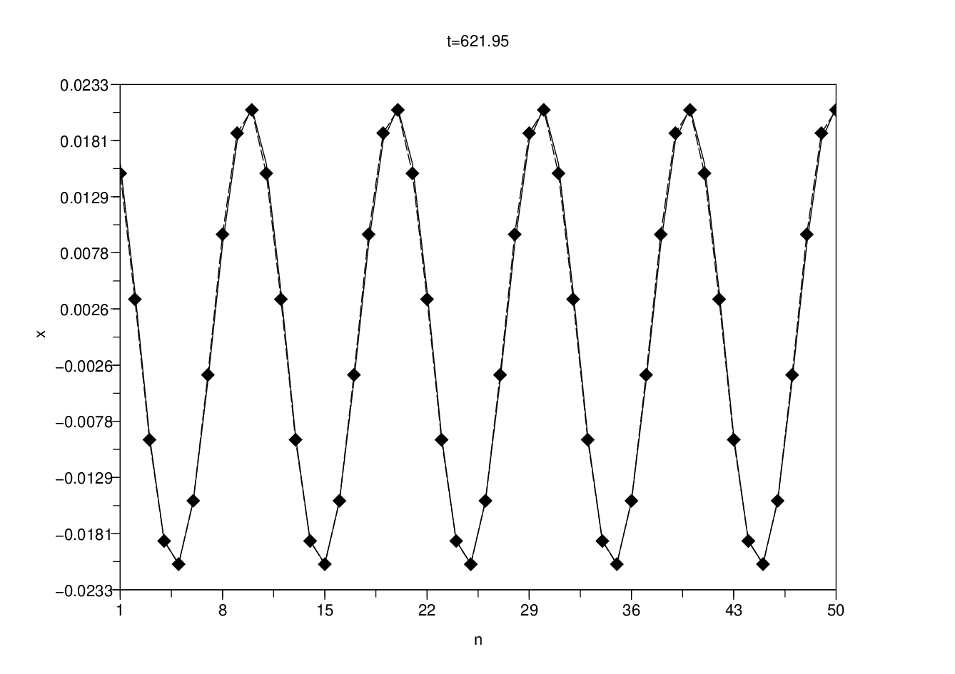
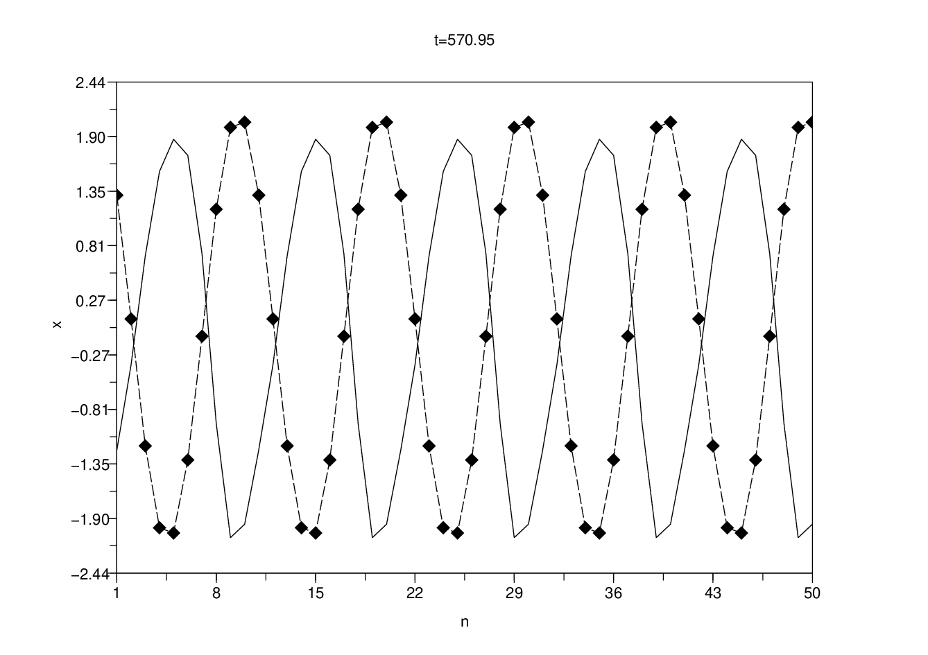
We begin by computing periodic travelling waves in the small amplitude regime in which the weakly nonlinear analysis of section 2.1 has been performed. We normalize the travelling wave solution (28) by fixing $R=1$ , so that $a=2\epsilon$ in ansatz (31). For the first numerical run, we choose (31) as an initial condition, with $\phi=0$ , $q=\pi/5$ and $\omega_{\rm{tw}}=1.01$ , which yields $a\approx 2.10^{-2}$ in the nonlinear dispersion relation (32). These parameter values correspond to a weakly-nonlinear regime, since the maximal value of the nonlinear interaction forces $|V_{0}^{\prime}(x_{n+1}^{\rm{tw}}-x_{n}^{\rm{tw}})|$ estimated with (31) is close to $a^{3/2}/2$ , which corresponds to seven percent of the maximal linear restoring force $a$ . As shown by figure 5 (left plot), the agreement between the exact and approximate solutions is excellent, even over long times corresponding to $100$ multiples of the wave period $T_{\rm{tw}}=2\pi/\omega_{\rm{tw}}$ . More precisely, the relative error between exact and approximate solutions (measured with the supremum norm) is less than five percent at the final time of computation (figure 5, right plot). These results show that the wave profile remains almost sinusoidal. However, nonlinear effects cannot be neglected on the timescales we have considered, because they still affect the wave velocities. This appears clearly in the right plot of figure 6, which compares the exact and approximate solutions to the linear wave with same amplitude $a$ and frequency $\omega=1<\omega_{\rm{tw}}$ . This wave has a lower velocity than the exact solution, so that it becomes approximately out of phase at time $t_{0}=333.7$ . Nonlinear selection of the wave velocity is correctly captured by the DpS equation, since the graphs of the exact and approximate solutions are almost superposed.

In a second numerical run, we modify the previous initial condition by setting

A_{n}(0)=(1+\rho_{n}^{(1)})\,\cos{(qn)}-i\,(1+\rho_{n}^{(2)})\,\sin{(qn)},

(75)

where $\rho_{n}^{(1)},\rho_{n}^{(2)}\in[-1/2,1/2]$ are uniformly distributed random variables. The mismatch between exact and approximate solutions increases significantly compared to figure 5 (see figure 6, left plot), but the approximation remains very satisfactory given the large time interval considered. A better agreement between the exact and approximate solutions could probably be achieved by taking into account the higher order correction $R_{n}$ to (11) provided by (18). Besides the comparison between exact and approximate solutions, this numerical experiment reveals the stability of the corresponding travelling waves of equations (1) and (10), at least over $100$ periods of the linear oscillators (however instabilities might occur on longer timescales). As we shall see later, fast modulational instabilities can show up for other choices of wavenumbers $q$ .

Next we again choose ansatz (31) with $q=\pi/5$ as an initial condition, but increase the frequency up to $\omega_{\rm{tw}}=1.1$ , which yields $a\approx 2.11$ in (32). In that case, the maximal values of the nonlinear interaction force and the linear restoring force estimated with (31) are of the same order, i.e. this initial condition should correspond to a fully nonlinear regime. As shown by figure 7, the initial condition still generates a periodic travelling wave that is qualitatively well described by the DpS equation. Quite surprisingly, the waveform remains nearly sinusoidal and close to the ansatz (31) (see figure 8). However the ansatz doesn’t accurately describe the wave velocity, as revealed by the shift between the exact and approximate solutions.

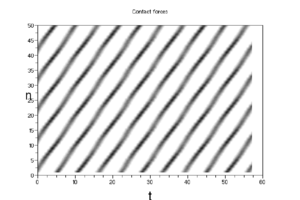
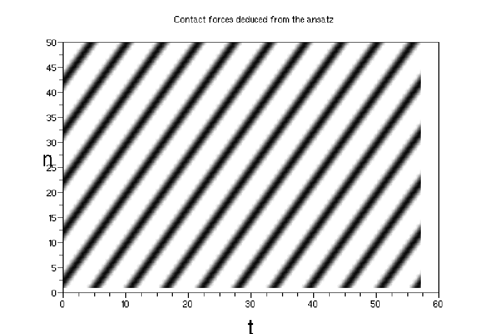
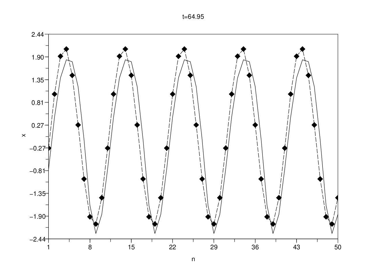
In the next computation we keep the same parameter values except we increase the frequency up to $\omega_{\rm{tw}}=1.5$ , so that $a\approx 52.9$ . This correspond to a highly nonlinear regime, where one can expect that the DpS equation will not properly describe the dynamics of (1). The two plots of figure 9 reveal indeed notable differences between the travelling wave patterns of the exact and approximate solutions. The initial condition generates in fact a pulsating travelling wave, showing internal oscillations that appear as spots along the wavefronts of figures 9 and 10. This internal breathing appears at the beginning of the simulation (around $t=1$ ) and releases some energy in the form of small amplitude travelling waves with lower velocity. These waves subsequently collide with the main travelling wave, generating travelling waves with negative velocities. These phenomena are absent in the DpS equation as shown by the right plot of figure 9. In addition the wave profile is not any more sinusoidal (see figure 10, right plot).

As a conclusion, we have seen that the initial condition obtained with ansatz (31) and $q=\pi/5$ generates a stable travelling wave that is qualitatively well described by the DpS equation if one avoids the highly nonlinear regime. Moreover, in the weakly nonlinear regime the DpS equation describes the travelling wave with excellent precision.

4.2. Modulational instability and breathers

In what follows we perform the same kind of simulations but increase the wavenumber $q$ above $\pi/2$ , which yields a completely different dynamical behaviour corresponding to modulational instability. We first determine an unperturbed initial condition using ansatz (31)-(32) with $q=4\pi/5$ and $\omega_{\rm{tw}}=1.1$ , which corresponds to a small amplitude $\epsilon\approx 3,\!8.10^{-3}$ in (30) (as above the travelling wave solution (28) is normalized by fixing $R=1$ ). Then we perturb this initial condition as indicated in (75), where $\rho_{n}^{(1)},\rho_{n}^{(2)}\in[-0.1,0.1]$ denote uniformly distributed random variables. The phenomenon of modulational instability is illustrated by figures 11 and 12. The envelope of the initial condition (figure 11, left plot) localizes after some transcient time, yielding larger oscillations of some beads corresponding to discrete breathers (figure 11, right plot). The modulational instability yields a disordered train of travelling breathers that propagate along the lattice as shown by figure 12. The DpS equation describes this modulational instability quite well (compare the two plots of figure 12), and even reproduces fine details like the crossing of two breathers at $t\approx 330$ .

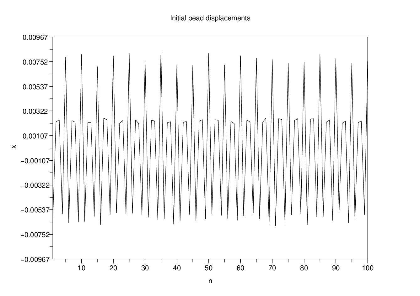
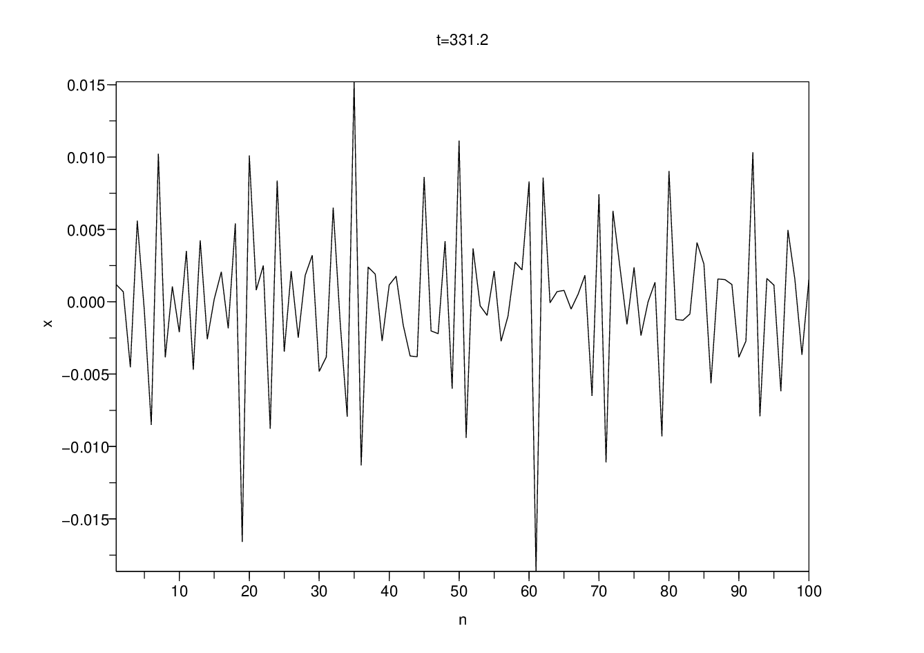
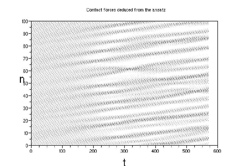
The average velocity of the travelling breathers generated near the onset of instability depends on the wavenumber of the unstable travelling wave. When $q$ is equal or close to $\pi$ ( $q=\pi$ corresponding to binary oscillations), one typically observes static breathers that remain pinned to some lattice sites over long times. This phenomenon is illustrated by figures 13 and 14, which correspond to the case $q=\pi$ , $\omega_{\rm{tw}}=1.1$ and $\rho_{n}^{(1)},\rho_{n}^{(2)}\in[-0.5,0.5]$ . The DpS equation provides a good qualitative picture of the instability (compare the two plots of figure 14). It is able to reproduce some complex phenomena like the interaction and subsequent merging of two close static breathers, at $t\approx 223$ . However the local dynamics after the two breathers have merged is not well described by the DpS equation, since more energy is released at the collision site for the exact solution than with the approximate solution. This may be the sign that higher harmonics neglected by ansatz (11) come into play during the merging phase, or may simply originate from sensitiveness of the collision result to relative phases and breather positions.

In the above space-time diagrams, travelling and static breathers appear as grey lines due to their internal breathing motion. These oscillations are more visible on figure 15, where static breathers with different amplitudes and spatial extentions are shown.

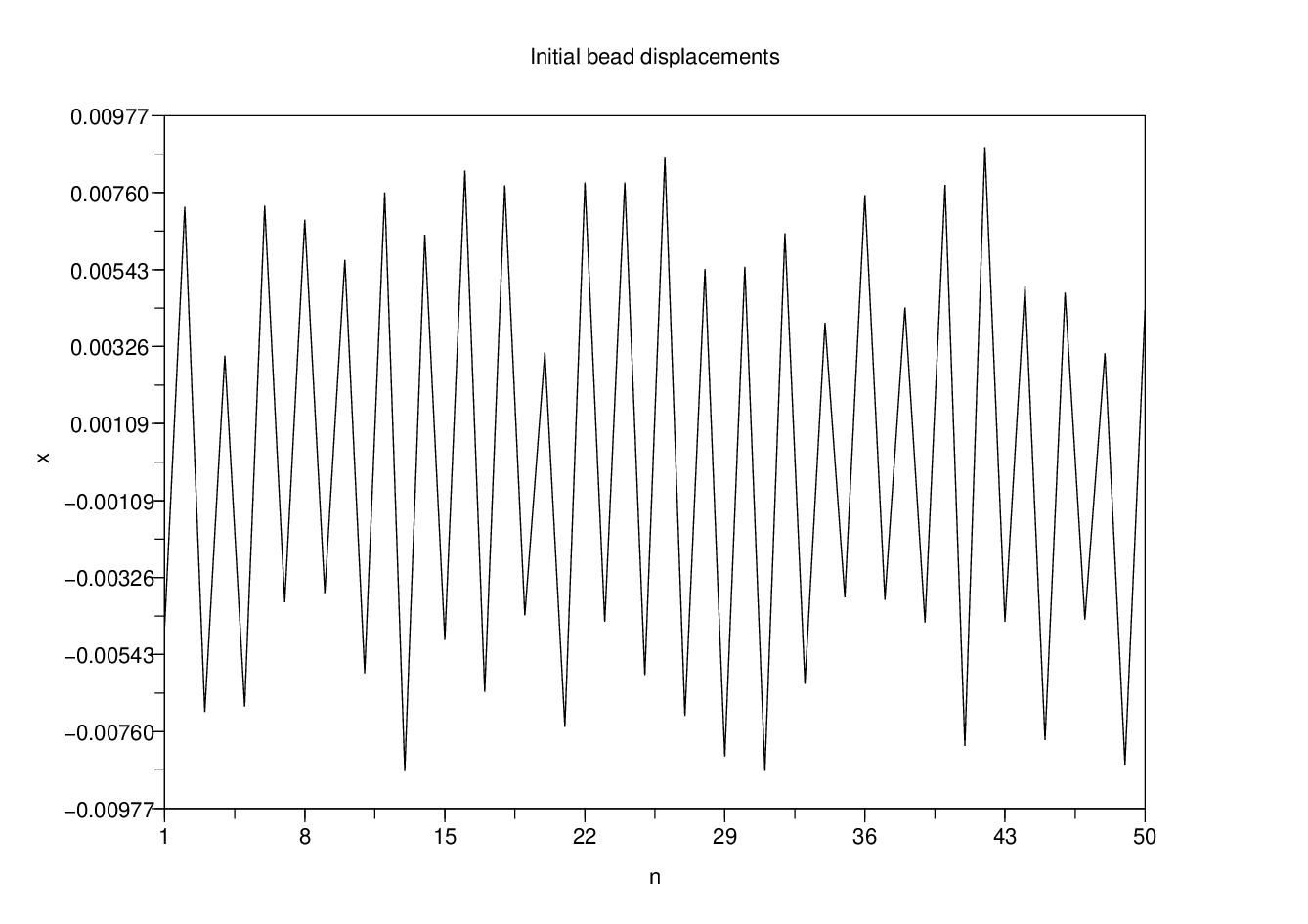
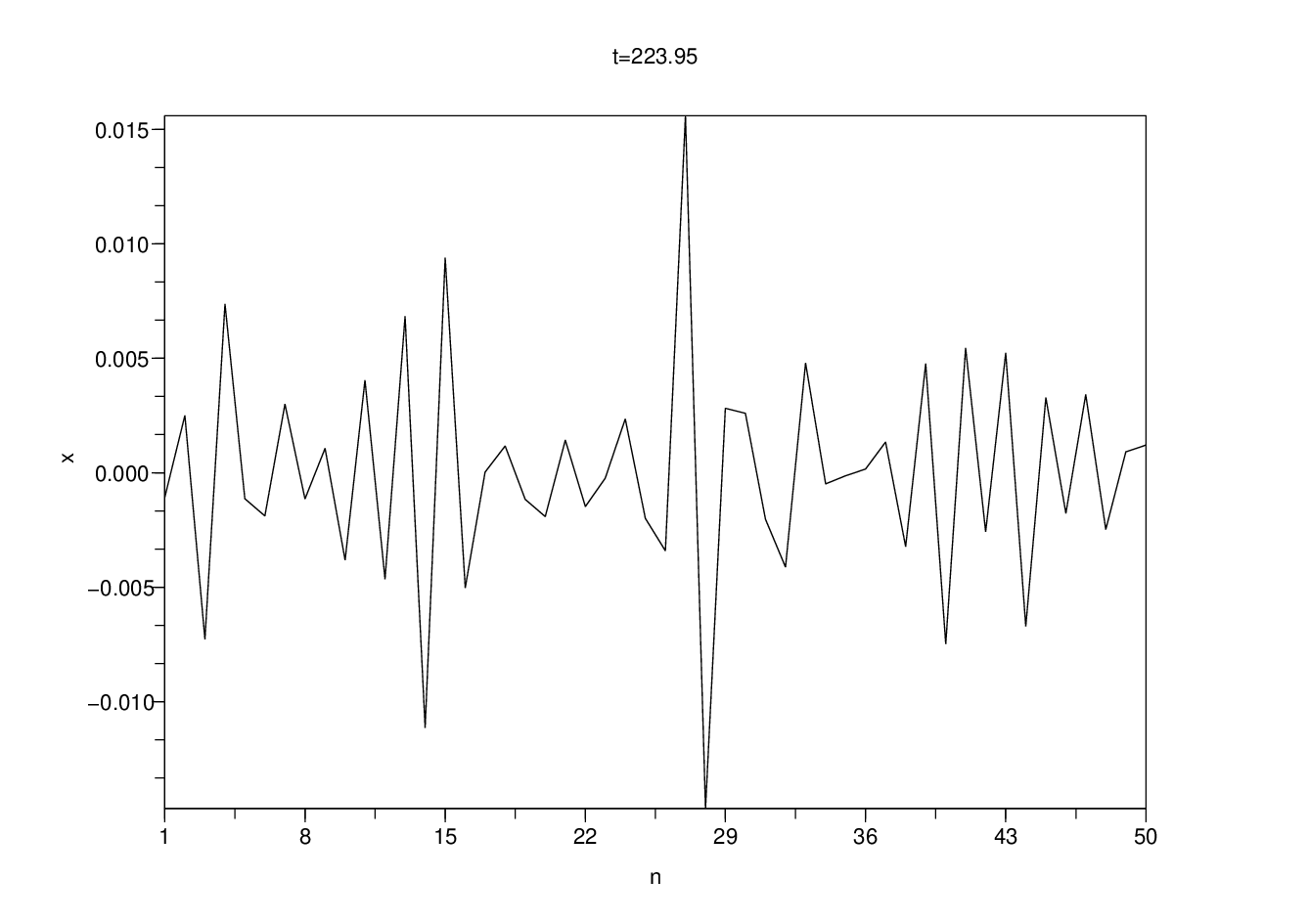
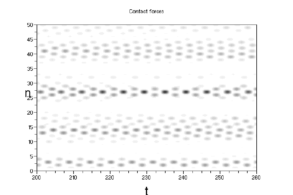
During the modulational instability, only a part of the modes are initially amplified. In order to analyze how the DpS equation is able to reproduce this phenomenon, we now study the time evolution of the spatial Fourier transform of $\{x_{n}(t)\}$ . As previously we consider periodic boundary conditions $x_{n+N}(t)=x_{n}(t)$ , but increase the number of particles to $N=200$ in order to achieve a better spectral resolution. Considering the discretization of the spectral band $[-\pi,\pi]$ given by $\Gamma_{\ast}=\frac{2\pi}{N}\cdot\{-\frac{N}{2}+1,\ldots,\frac{N}{2}\}$ and defining the discrete Fourier transform

\hat{x}_{k}(t)=\sum_{n=0}^{N-1}{x_{n}(t)\,e^{-i\,n\,k}},\ \ \ k\in\Gamma_{\ast},

we have

x_{n}(t)=\frac{1}{N}\,\sum_{k\in\Gamma_{\ast}}{\hat{x}_{k}(t)\,e^{i\,n\,k}}.

We compare the time evolution of the magnitude of the Fourier transform $|\hat{x}_{k}(t)|$ for the exact and approximate solutions, for initial travelling wave profiles perturbed by random noise. The unperturbed initial condition is determined using ansatz (31)-(32), for $\omega_{\rm{tw}}=1.1$ and different wavenumbers $q$ that determine the amplitude $\epsilon=a/2$ in (30). We perturb this initial condition as indicated in (75), where $\rho_{n}^{(1)},\rho_{n}^{(2)}$ are random variables generated from the Gaussian distribution with mean $0$ and standard deviation $0,\!5.10^{-2}$ .

Figure 16 compares the spectra of the exact and approximate solutions for $q=4\pi/5$ . At $t=106.7$ (first row), the two peaks at $k=\pm q$ correspond to the periodic travelling wave generated by the initial condition. Two second harmonics at $k=\pm 2(q-\pi)$ are visible for the exact solution and are absent for the approximate one (these harmonics are generated at early times of the simulation even in the absence of noise). As time further increases, a band of unstable modes grows in amplitude at both sides of $k=\pm q$ . The unstable bandwidths and most unstable wavenumbers of the exact and approximate solutions are quite close (compare the plots at $t=399.95$ , third row), but the approximate solution overestimates the initial growth rate (compare the plots at $t=253.45$ , second row). Both for the exact and approximate solutions, a breathing of the spectrum near $k=\pm\pi$ settles progressively. The plots at the fourth row show quite similar spectral distributions of the exact solution at $t=541.95$ and of the approximate one at $t=543.7$ (we have slightly shifted time to compensate a phase-shift in the spectral breathing). As a conclusion, the DpS equation describes quite accurately the modulational instability of the travelling wave with $q=4\pi/5$ in the weakly nonlinear regime.

In contrast with the above results, we describe below two situations in which the DpS equation gives incorrect results on the stability or dynamical properties of travelling waves.

The first one corresponds to a simple instability threshold effect. For $q=\pi/2$ and below, we haven’t observed modulational instabilities both for the DpS equation and system (1) in the weakly nonlinear regime. However, in both models we have found thresholds for the modulational instability at slightly different critical values of $q$ near $\pi/2$ . This is illustrated by figure 17, where the magnitudes of the spatial Fourier transforms of the exact and approximate solutions are plotted at $t=913.7$ ( $160$ time periods of the initial periodic travelling wave) for different values of $q$ near $\pi/2$ . As shown by the two plots at the first row, small amplitude travelling waves with $q=52\pi/100$ are unstable both for system (1) and the DpS approximation. When $q$ decreases to $q=51\pi/100$ , the modulational instability persists for the DpS approximation, but it does not occur (or may occur extremely slowly) for system (1) (see plots at the second row). The third row of figure 17 provides the spectra for $q=\pi/2$ , showing no trace of modulational instability. In addition to the main peaks, one can see second harmonics at $k=\pm\pi$ in the exact solution spectrum, and a small noisy background (more important for the exact solution) that follows from an energy cascade between modes. As a conclusion, these computations reveal that system (1) and the DpS approximation yield slightly different instability thresholds for the wavenumber $q$ , and consequently the DpS approximation does not correctly describe the dynamics when $q$ is chosen between the two critical values.

As second situation in which the DpS approximation breaks down is described in figure 18. For $q=57\pi/100$ , the travelling wave develops a modulational instability both in system (1) and the DpS equation, but the two models display different transitory dynamical behaviours. This originates from two small harmonics appearing in the spectrum of the exact solution at early times of the simulation, more precisely a second harmonic at $k=\pm 2(q-\pi)$ and a third harmonic at $k=\pm(3q-2\pi)$ . As previously these peaks are absent in the spectrum of the approximate solution. Here the difference with respect to figures 16 and 17 is that these small peaks fall inside the bands of modes amplified by modulational instability, and their amplitude grows with time (the second harmonic dominates the third one at the beginning of the simulation, but their amplitudes become comparable arount $t=150$ ). This results in the spectra shown in figure 18, where two additional large amplitude oscillating peaks are present in the spectrum of the exact solution at $t=344.95$ (upper left plot) and absent for the approximate solution (upper right plot). The two middle plots show the bead displacements for the exact solution at two different times, revealing a large scale standing wave that strongly modulates the basic pattern. The lower plot corresponds to the approximate solution given by the DpS equation, which is very weakly modulated and fails to reproduce the correct transitory dynamics of (1) in the present situation. However, in both models broad bands of unstable modes become slowly amplified at larger times by modulational instability (this appears clearly after $t=600$ for system (1) and $t=700$ for the DpS equation), and around $t=900$ the bead displacements show rather similar features in both cases.

4.3. Localized initial conditions

In section 4.2 we have seen that the modulational instability of certain travelling waves generates travelling or static breathers, a phenomenon which can be captured by the DpS equation. In what follows we illustrate with a few examples how the DpS equation approximates the evolution and interaction of these localized structures.

We start by generating single breathers similar to the ones that result from the modulational instability of the $q=\pi$ mode. For this purpose, we consider the spatially antisymmetric homoclinic solution $\{a_{n}\}$ of (37) represented in figure 4 (bottom left plot), the associated breather solution of (24)

A_{n}(\tau)=\frac{1}{2}\,{\mu}^{\frac{1}{\alpha-1}}\,{a}_{n}\,e^{i\,(\omega_{\rm{sw}}-1)\,\tau},\ \ \ \mu=(\omega_{\rm{sw}}-1)\,2^{\alpha}\tau_{0}>0,

(76)

and the corresponding breather ansatz (41). Using the initial condition determined by (41), we integrate (1) numerically. Computations are performed for a chain of $N=50$ particles with periodic boundary conditions.

The results are shown in figure 19 for different amplitudes of the initial breather profile obtained by varying $\mu$ . The first case corresponds to $|x_{N/2+1}(0)|\approx 9,\!7.10^{-3}$ , i.e. $\omega_{\rm{sw}}\approx 1.1$ (initial condition shown in the top left plot). By construction, the profile of the approximate solution given by the DpS equation remains similar to the top left plot for all times, just oscillating periodically in time. One observes the same qualitative behaviour for the exact solution. As shown by the top right plot, the profiles of the exact solution at $t=569.4$ (continuous line) and the approximate solution at $t=565.95$ (dots) are very close (we compare both profiles with a small time-shift, because the exact and approximate solutions develop a half-period phase-shift after approximately $83$ breather periods). These results show the efficiency of approximation (41) on large time intervals of the order of $100$ multiples of the breather period. As shown by the bottom left plot, this localized $3$ -sites breather solution qualitatively corresponds to the central breather forming in figure 15. In the second case, the initial profile has a larger amplitude $|x_{N/2+1}(0)|\approx 0.34$ , which corresponds to $\omega_{\rm{sw}}\approx 1.6$ . The bottom right plot (bead displacements at $t=293.2$ ) show that small dispersive waves are emitted by the exact solution. On the contrary, the DpS equation does not yield any dispersion in that case, only time-periodic oscillations of the profile given by the initial condition.

Remark 6.

We obtain qualitatively similar results with the spatially symmetric homoclinic solution $\{a_{n}\}$ of (37) (figure 4, top left plot), except the exact solution rapidly develops a slight asymmetry which is absent in the approximate solution. This is due to the fact that (1) does not possess the invariance $x_{n}\rightarrow x_{-n}$ , whereas (10) has the invariance $A_{n}\rightarrow A_{-n}$ . The asymmetry of the approximate solution could be recovered by taking into account the higher order term $R_{n}$ present in (18).

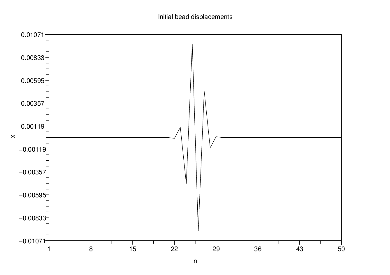
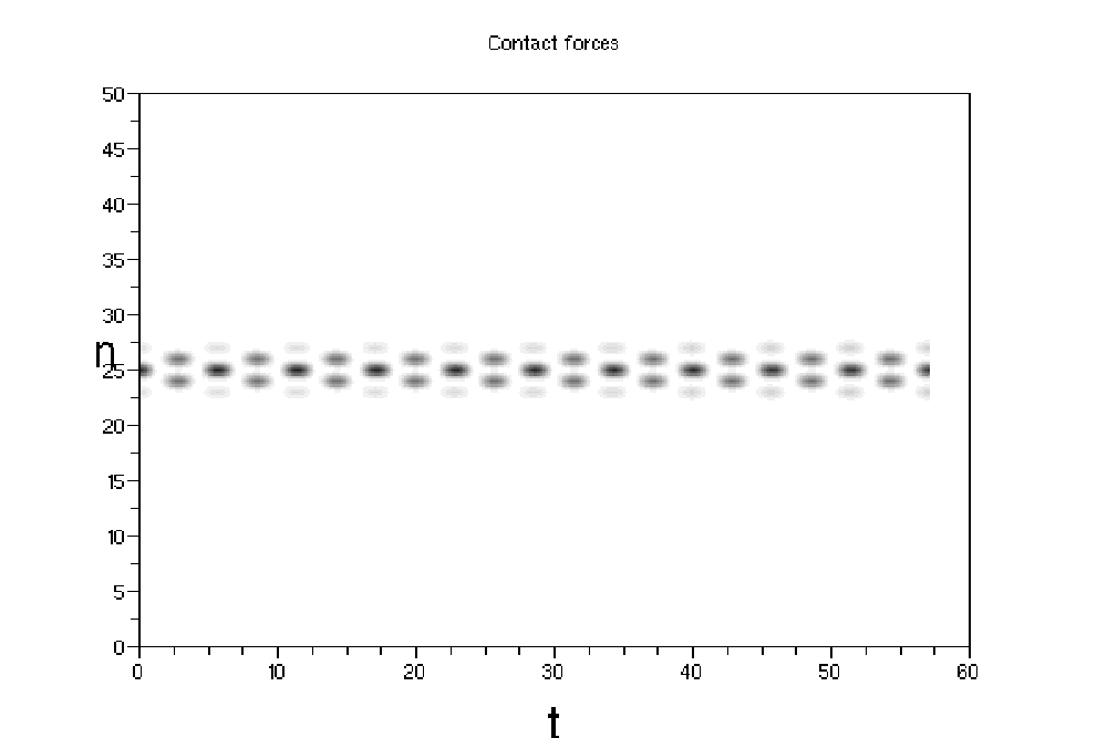
The above computation shows that the DpS equation can approximate single breather solutions of (1) provided their amplitude is sufficiently small, i.e. their frequency sufficiently close to $1$ . Now let us illustrate how the DpS equation accounts for the interaction of small amplitude breathers, on long times scales up to $600$ breather periods. Initial conditions for (1) are generated using the ansatz (41) with $\omega_{\rm{sw}}\approx 1.1$ , for initial envelopes $\{a_{n}\}$ that do not correspond to exact solutions of equation (37). The DpS equation is initialized by setting $\tau=0$ in (76).

The left side plots of figure 20 correspond to initial displacements almost compactly supported on $12$ lattice sites, modulating binary oscillation with amplitude close to $0.016$ (top plot). Initial velocities are set to $0$ . The spatiotemporal evolution of the interaction forces is shown for equation (1) (middle plot) and the DpS approximation deduced from ansatz (11) (bottom plot). In both cases, the initial packet splits into a static breather and two pairs of breathers travelling slowly in opposite directions. Further crossings of the pulses occur, with some interactions resulting in small phase shifts or velocity changes. The global sequence of collisions is different for the exact and approximate solutions (because collisions result in differences that accumulate with time), but these computations show nevertheless a good qualitative agreement between the exact and approximate dynamics.

The right side plots of figure 20 are obtained for initial displacements corresponding to two small amplitude static breathers initially separated by one lattice site (top plot), with amplitude close to $0.01$ and zero initial velocities. Merging of the two breathers occurs after a long transcient, both for the exact (middle plot) and approximate (bottom plot) solutions. However this occurs at largely different times, around $175$ multiples of the breather period for the exact solution, and twice more for the approximate solution. In that case, the DpS approximation gives consequently a good qualitative picture of the slow interaction of the two breathers, but is quantitatively not satisfactory to predict the finite lifetime of the two-breather bound state.

Let us end this section with some remarks concerning boundary conditions. So far we have computed discrete breathers in chains of $N$ beads with $N\geq 50$ and periodic boundary conditions. From an experimental point of view, system (1) corresponds in that case to a closed ring of $N$ beads, where $N$ must be large enough in order to avoid curvature effects. However most experiments with Newton’s cradles have been performed with a small number of beads arranged linearly, which corresponds to system (1) with free end boundary conditions. It is important to stress that discrete breathers can be also generated in this context, as shown by figure 21. The left plots show displacements in a chain of $10$ beads at different times, obtained by numerical integration of system (1) with free end boundary conditions. The results show the existence of a spatially antisymmetric breather involving mainly $4$ beads. The initial condition is generated using the same method and parameter values as for the small amplitude breather of figure 19 (top left plot), except we use free end boundary conditions in the stationary DpS equation (37) to compute the breather ansatz (41). The right plots show the approximate solution (41) deduced from the DpS equation. The latter agrees very well with the exact solution, except both differ by a phase-shift that is increasing with time.

5. Conclusion

Although Newton’s cradle has a long history which dates back to the $17$ th century [40], it is still considered as a benchmark in recent research at the cutting edge of impact mechanics [52, 53]. Moreover, this system turns out to be very interesting from the modern perspective of nonlinear science. It allows a simple experimental realization of three nontrivial nonlinear effects, namely fully nonlinear dispersion [64], a limited smoothness of nonlinear interactions and their unilaterality. The last two aspects are still rather unexplored in the context of nonlinear waves. As we have seen in this paper, these different features require to revisit several classical topics, i.e. local bifurcations of periodic waves, modulation equations with fully nonlinear dispersion described by discrete $p$ -Laplacians, modulational instability and the bifurcation and interaction of discrete breathers. These topics are obviously very broad, and our work is only a first step towards a better understanding of these questions in a new context.

From an analytical point of view, we know by theorem 1 the existence of exact periodic travelling waves of (1) close to small amplitude approximate solutions given by the DpS equation. The above numerical simulations have revealed that the DpS equation has in fact a much wider applicability. Indeed, it captures other important features of the dynamics of (1) in the weakly nonlinear regime, namely modulational instabilities, the existence of static and travelling breathers, and several types of interactions of these localized structures. An interesting open question is to justify mathematically this close relation between the dynamics of (1) and the DpS equation, for well-prepared initial conditions close to (11) at $t=0$ and large finite time intervals. Interestingly, such results have been proved in a different context for the DNLS equation (12), where this system is used to approximate solutions of the Gross-Pitaevskii equation with a periodic potential (see [62] and references therein).

In the same spirit, it has been shown recently [33, 34, 8, 66] that the continuum cubic nonlinear Schrödinger (NLS) equation (which can be derived in continuum limits of the DNLS equation) approximates the evolution of well-prepared initial data in many nonlinear lattices. It would be interesting to know if the above results extend to equation (27) or its generalizations to finite-wavelength continuum limits of the DpS equation. Our situation is more complex than in the NLS case, due to the limited smoothness of (1) at the origin, and because the Cauchy problem for (27) seems delicate to analyze. In addition, the analysis of continuum limits of the DpS equation may provide interesting informations on the nonlinear waves of (1), e.g. additional explicit approximate solutions. In particular, explicit compactly supported travelling or standing waves have been found recently in some variants of equation (27) that were formally introduced in [74, 75] and in a continuum limit of the D-QLS equation [64] (see remark 1 p.1). Such solutions may also exist for continuum limits of the DpS equation, and may accurately approximate the almost compactly supported breathers computed in section 2.2 and 4.3.

Interesting open problems related to discrete breathers in Newton’s cradle (1) and the DpS equation concern the analytical proof of their existence, their numerical continuation, as well as their stability, movability and interaction properties. It will be interesting to compare their collision properties in both models, a problem which requires a statistical treatment due to its sensitiveness to relative phases and breather positions [9]. In the context of impact mechanics, discrete breathers may be used for stringent numerical tests of multiple impact laws in model (1). They may be also useful for practical purposes, since granular chains are interesting devices for the design of shock absorbers (see [69, 25] and references therein), and the possibility might exist to trap a part of the energy of an incident wave into static breathers in an efficient way. However, before comparing our theoretical results to experiments it will be necessary to evaluate the impact of dissipation [12] and spatial inhomogeneities on the nonlinear waves we have considered.

Another interesting question is the study of the modulational instability of travelling waves in the DpS equation and its more exhaustive comparison with modulational instabilities in system (1). One of the great interests of the DpS equation stems from the fact that the first part of the problem can be worked out analytically, as done in reference [15] for the DNLS equation. In addition a more precise numerical study of modulational instabilities in Newton’s cradle and the DpS equation (comparing e.g. the most unstable modes in both models) will require statistics on power spectra of perturbations.

More generally, one can wonder if the DpS equation or higher-dimensional extensions could capture some general features of nonlinear waves in more general granular media. Interesting questions related to nonlinear waves arise in this context, e.g. the possibility of earthquake triggering by travelling or standing waves in granular fault gouges [47].

Acknowledgements: The author acknowledges stimulating discussions with V. Acary, B. Brogliato, P. Kevrekidis and M. Peyrard.

References

[1] M. Abramowitz and I.A. Stegun, eds. Handbook of Mathematical Functions, National Bureau of Standards, 1964 (10th corrected printing, 1970), www.nr.com.
[2] V. Acary and B. Brogliato. Concurrent multiple impacts modelling: Case study of a 3-ball chain, Proc. of the MIT Conference on Computational Fluid and Solid Mechanics, 2003 (K.J. Bathe, Ed.), Elsevier Science, 1836-1841.
[3] K. Ahnert and A. Pikovsky. Compactons and chaos in strongly nonlinear lattices, Phys. Rev. E 79 (2009), 026209.
[4] G.L. Alfimov, V.A. Brazhnyi and V.V. Konotop. On classification of intrinsic localized modes for the discrete nonlinear Schrödinger equation, Physica D 194 (2004), 127-150.
[5] S. Aubry. Anti-integrability in dynamical and variational problems, Physica D 86 (1995), 284-296.
[6] S. Aubry, G. Kopidakis and V. Kadelburg. Variational proof for hard discrete breathers in some classes of Hamiltonian dynamical systems, Discrete Contin. Dyn. Syst. Ser. B 1 (2001), 271-298.
[7] D. Bambusi and A. Ponno. On metastability in FPU, Comm. Math. Phys. 264 (2006), 539-561.
[8] D. Bambusi, A. Carati and T. Penati. Boundary effects on the dynamics of chains of coupled oscillators, Nonlinearity 22 (2009), 923-945.
[9] O. Bang and M. Peyrard. Generation of high-energy localized vibrational modes in nonlinear Klein-Gordon lattices, Phys. Rev. E 53 (1996), 4143-4152.
[10] N. Boechler, G. Theocharis, S. Job, P.G. Kevrekidis, M.A. Porter and C. Daraio. Discrete breathers in one-dimensional diatomic granular crystals, Phys. Rev. Lett. 104 (2010), 244302.
[11] D.K. Campbell et al, editors. The Fermi-Pasta-Ulam problem : the first $50$ years, Chaos 15 (2005).
[12] R. Carretero-González, D. Khatri, M.A. Porter, P.G. Kevrekidis and C. Daraio. Dissipative solitary waves in granular crystals, Phys. Rev. Lett. 102 (2009), 024102.
[13] V. Ceanga and Y. Hurmuzlu. A new look at an old problem : Newton’s cradle, J. Appl. Mech. 68 (2001) 575-584.
[14] A. Chatterjee. Asymptotic solutions for solitary waves in a chain of elastic spheres, Phys. Rev. E 59 (1999), 5912-5918.
[15] I. Daumont, T. Dauxois and M. Peyrard. Modulational instability : first step towards energy localization in nonlinear lattices, Nonlinearity 10 (1997), 617-630.
[16] W. Dreyer, M. Herrmann and A. Mielke. Micro-macro transition in the atomic chain via Whitham’s modulation equation, Nonlinearity 19 (2006), 471-500.
[17] W. Dreyer and M. Herrmann. Numerical experiments on the modulation theory for the nonlinear atomic chain, Physica D 237 (2008), 255-282.
[18] J.C. Eilbeck and M. Johansson. The discrete nonlinear Schrödinger equation - $20$ years on. In : L. Vazquez, R.S. MacKay, M-P. Zorzano, editors, Conference on Localization and Energy Transfer in Nonlinear Systems, p.44, World Scientific (2003).
[19] J.M. English and R.L. Pego. On the solitary wave pulse in a chain of beads, Proc. Amer. Math. Soc. 133, n. 6 (2005), 1763-1768.
[20] A.M. Filip and S. Venakides. Existence and modulation of traveling waves in particle chains, Comm. Pure Appl. Math. 52 (1999), 693-735.
[21] S. Flach. Conditions of the existence of localized excitations in nonlinear discrete systems, Phys. Rev. E 50 (1994), 3134-3142.
[22] S. Flach. Existence of localized excitations in nonlinear Hamiltonian lattices, Phys. Rev. E 51 (1995), 1503-1507.
[23] S. Flach, J. Dorignac, A.E. Miroshnichenko and V. Fleurov. Discrete breathers close to the anticontinuum limit : existence and wave scattering, Int. J. Mod. Phys. B 17 (2003), 3996-4002.
[24] S. Flach and A. Gorbach. Discrete breathers : advances in theory and applications, Physics Reports 467 (2008), 1-116.
[25] F. Fraternali, M. A. Porter, and C. Daraio. Optimal design of composite granular protectors, Mech. Adv. Mat. Struct. 17 (2010), 1-19.
[26] G. Friesecke and R.L. Pego. Solitary waves on FPU lattices : I. Qualitative properties, renormalization and continuum limit, Nonlinearity 12 (1999), 1601-1627.
[27] G. Friesecke and R.L. Pego. Solitary waves on FPU lattices : II. Linear implies nonlinear stability, Nonlinearity 15 (2002), 1343-1359.
[28] G. Friesecke and R.L. Pego. Solitary waves on FPU lattices : III. Howland-type Floquet theory, Nonlinearity 17 (2004), 207-227.
[29] G. Friesecke and R.L. Pego. Solitary waves on FPU lattices : IV. Proof of stability at low energy, Nonlinearity 17 (2004), 229-251.
[30] G. Friesecke and J.A Wattis. Existence theorem for solitary waves on lattices, Commun. Math. Phys. 161 (1994), 391-418.
[31] G. Fu. An extension of Hertz’s theory in contact mechanics, J. Appl. Mech. 74 (2007), 373-375.
[32] G. Gallavotti, editor. The Fermi-Pasta-Ulam Problem. A Status Report, Lecture Notes in Physics 728 (2008), Springer.
[33] J. Giannoulis and A. Mielke. The nonlinear Schrödinger equation as a macroscopic limit for an oscillator chain with cubic nonlinearities, Nonlinearity 17 (2004), 551-565.
[34] J. Giannoulis and A. Mielke. Dispersive evolution of pulses in oscillator chains with general interaction potentials, Discrete Contin. Dyn. Syst. Ser. B 6 (2006), 493-523.
[35] M. Herrmann. Unimodal wave trains and solitons in convex FPU chains, arXiv:0901.3736v1 (2009). To appear in Proc. Roy. Soc. Edinburgh A.
[36] E. J. Hinch and S. Saint-Jean. The fragmentation of a line of ball by an impact, Proc. R. Soc. London, Ser. A 455 (1999), 3201-3220.
[37] A. Hoffman and C.E. Wayne. Counter-propagating two-soliton solutions in the Fermi-Pasta-Ulam lattice, Nonlinearity 21 (2008), 2911-2947.
[38] A. Hoffman and C.E. Wayne. A simple proof of the stability of solitary waves in the Fermi-Pasta-Ulam model near the KdV limit (2008), arXiv:0811.2406v1.
[39] A. Hoffman and C.E. Wayne. Asymptotic two-soliton solutions in the Fermi-Pasta-Ulam model, J. Dyn. Diff. Equat. 21 (2009), 343-351.
[40] S. Hutzler, G. Delaney, D. Weaire and F. MacLeod. Rocking Newton’s cradle, Am. J. Phys. 72, n.12 (2004), 1508-1516.
[41] G. Iooss. Travelling waves in the Fermi-Pasta-Ulam lattice, Nonlinearity 13 (2000), 849-866.
[42] G. Iooss and G. James. Localized waves in nonlinear oscillator chains, Chaos 15 (2005), 015113.
[43] G. James. Existence of breathers on FPU lattices, C. R. Acad. Sci. Paris, Ser. I 332 (2001), 581-586.
[44] G. James. Centre manifold reduction for quasilinear discrete systems, J. Nonlinear Sci. 13 (2003), 27-63.
[45] J.-Y. Ji and J. Hong. Existence criterion of solitary waves in a chain of grains, Phys. Lett. A 260 (1999), 60-61.
[46] K.L. Johnson. Contact mechanics, Cambridge Univ. Press, 1985.
[47] P.A. Johnson and X. Jia. Nonlinear dynamics, granular media and dynamic earthquake triggering, Nature 437 (2005), 871-874.
[48] L.A. Kalyakin. Long wave asymptotics. Integrable equations as asymptotic limits of non-linear systems., Russian Math. Surveys 44 (1989), 3-42.
[49] Yu. S. Kivshar and M. Peyrard. Modulational instabilities in discrete lattices, Phys. Rev. A 46 (1992), 3198-3205.
[50] Yu. S. Kivshar. Intrinsic localized modes as solitons with a compact support, Phys. Rev. E 48 (1993), R43-R45.
[51] L.D. Landau, E.M. Lifshitz, A.M. Kosevich and L.P. Pitaevskii. Theory of Elasticity, Third Edition (Theoretical Physics, Vol 7), Butterworth-Heinemann (1986).
[52] C. Liu, Z. Zhao and B. Brogliato. Frictionless multiple impacts in multibody systems. I. Theoretical framework. Proc. R. Soc. A-Math. Phys. Eng. Sci., 464 (2008), 3193-3211.
[53] C. Liu, Z. Zhao and B. Brogliato. Frictionless multiple impacts in multibody systems. II. Numerical algorithm and simulation results, Proc. R. Soc. A-Math. Phys. Eng. Sci., 465 (2009), 1-23.
[54] W. Ma, C. Liu, B. Chen and L. Huang. Theoretical model for the pulse dynamics in a long granular chain, Phys. Rev. E 74 (2006), 046602.
[55] R.S. MacKay and S. Aubry. Proof of existence of breathers for time-reversible or Hamiltonian networks of weakly coupled oscillators, Nonlinearity 7 (1994), 1623-1643.
[56] R.S. MacKay. Solitary waves in a chain of beads under Hertz contact, Phys. Lett. A 251 (1999), 191-192.
[57] A.M. Morgante, M. Johansson, G. Kopidakis and S. Aubry. Standing wave instabilities in a chain of nonlinear coupled oscillators, Physica D 162 (2002), 53-94.
[58] V.F. Nesterenko. Propagation of nonlinear compression pulses in granular media, J. Appl. Mech. Tech. Phys. 24 (1983), 733-743.
[59] V.F. Nesterenko, Dynamics of heterogeneous materials, Springer Verlag, 2001.
[60] A. Pankov and K. Pflüger. Travelling waves in lattice dynamical systems, Math. Meth. Appl. Sci. 23 (2000), 1223-1235.
[61] A. Pankov. Travelling waves and periodic oscillations in Fermi-Pasta-Ulam lattices, Imperial College Press, London, 2005.
[62] D. Pelinovsky and G. Schneider. Bounds on the tight-binding approximation for the Gross-Pitaevski equation with a periodic potential, J. Differential equations 248 (2010), 837-849.
[63] M. Porter, C. Daraio, I. Szelengowicz, E.B. Herbold and P.G. Kevrekidis, Highly nonlinear solitary waves in heterogeneous periodic granular media, Physica D 238 (2009), 666-676.
[64] P. Rosenau and S. Schochet. Compact and almost compact breathers: a bridge between an anharmonic lattice and its continuum limit, Chaos 15 (2005), 015111.
[65] G. Schneider and C.E. Wayne. Counter-propagating waves on fluid surfaces and the continuum limit of the Fermi-Pasta-Ulam model. In : B. Fiedler, K. Gröger and J. Sprekels, editors, International Conference on Differential Equations Appl. 5 (1998), n.1, 69-82.
[66] G. Schneider. Bounds for the nonlinear Schrödinger approximation of the Fermi-Pasta-Ulam system, Appl. Anal. 89 (2010), 1523-1539.
[67] H. Schwetlick and J. Zimmer. Solitary waves for nonconvex FPU lattices, J. Nonlinear Sci. 17 (2007), 1-12.
[68] K. Sekimoto. Newton’s cradle versus nonbinary collisions, Phys. Rev. Lett. 104 (2010), 124302.
[69] S. Sen, J. Hong, J. Bang, E. Avalos and R. Doney. Solitary waves in the granular chain, Physics Reports 462 (2008), 21-66.
[70] A.J. Sievers and J.B. Page. Unusual anharmonic local mode systems. In : G.K. Norton and A.A. Maradudin, editors, Dynamical Properties of Solids 7, Ch. 3, North-Holland, Amsterdam (1995).
[71] D. Smets and M. Willem. Solitary waves with prescribed speed on infinite lattices, J. Funct. Anal. 149 (1997), 266-275.
[72] D.A. Spence, Self-similar solutions to adhesive contact problems with incremental loading, Proc. Roy. Soc. Lond. Ser. A 305 (1968), 55-80.
[73] G. Theocharis, M. Kavousanakis, P.G. Kevrekidis, C. Daraio, M.A. Porter and I.G. Kevrekidis. Localized breathing modes in granular crystals with defects, Phys. Rev. E 80 (2009), 066601.
[74] Z. Yan. Envelope compactons and solitary patterns, Phys. Lett. A 355 (2006), 212-215.
[75] Z. Yan. Envelope compact and solitary pattern structures for the GNLS(m,n,p,q) equation, Phys. Lett. A 357 (2006), 196-203.

Nonlinear waves in Newton’s cradle and the discrete pp-Schrödinger equation

Abstract.

Key words and phrases:

2000 Mathematics Subject Classification

1. Introduction and main results

Theorem 1.

2. The DpS equation for modulated waves

2.1. Formal derivation and elementary properties

Remark 1.

2.2. Time-periodic travelling and standing waves

Remark 2.

Remark 3.

3. Proof of theorem 1

3.1. Fixed point problem for periodic travelling waves

3.2. Solution of the fixed point problem

Lemma 1.

Proof.

Theorem 2.

Proof.

Remark 4.

Remark 5.

3.3. Symmetries

4. Numerical comparison of the DpS model and Newton’s cradle

4.1. Approximation of stable travelling waves

4.2. Modulational instability and breathers

4.3. Localized initial conditions

Remark 6.

5. Conclusion

References

Nonlinear waves in Newton’s cradle and the discrete $p$ -Schrödinger equation