August 24, 2026
Fivebranes and resolved deformed manifolds
Jérôme Gaillard1 and Dario Martelli2
1Swansea University,
Singleton Park, Swansea SA2 8PP, United Kingdom
2 Department of Mathematics, King’s College, London
The Strand, London WC2R 2LS, United Kingdom
We study supergravity solutions corresponding to fivebranes wrapped on a three-sphere inside a holonomy manifold. By changing a parameter the solutions interpolate between a manifold with flux on a three-sphere and a distinct manifold with branes on another three-sphere. Therefore, these realise a geometric transition purely in the supergravity context. We can add D2 brane charge by applying a simple transformation to the initial solution and we obtain one-parameter deformations of warped holonomy backgrounds. These solutions suggest a connection between the Chern-Simons theory on the fivebranes and the field theory dual to D2 branes and fractional NS5 branes, transverse to the manifold .
1 Introduction
Calabi-Yau manifolds have played an important role in string theory for many years. For example, string theory compactified on a Calabi-Yau manifold gives rise to an effective four-dimensional theory with unbroken supersymmetry. In the context of the AdS/CFT correspondence [1], conical Calabi-Yau three-fold singularities equipped with a Ricci flat metric give rise to supersymmetric solutions of Type IIB string theory with an AdS5 factor [2, 3, 4, 5], thus providing precise gravity duals to a large class of supersymmetric field theories.
The simplest and most studied Calabi-Yau singularity in string theory is the conifold [6]. There are two distinct desingularisations of this, in which the singularity at the tip is replaced by a three-sphere or a two-sphere. These are referred to as deformation and resolution, respectively. The relevance of the transition between the resolved and deformed conifold in string theory was emphasised in [7]. The deformed conifold geometry underlies the Klebanov-Strassler solution [8], which is dual to a four-dimensional field theory displaying confinement. A different supergravity solution dual to a closely related field theory was discussed by Maldacena-Nuñez [9, 10]. This arises as the decoupling limit of a configuration of fivebranes wrapped on the two-sphere of the resolved conifold.
A solution of Type IIB supergravity that contains as special cases the Klebanov-Strassler and the Maldacena-Nuñez solutions was constructed in [11]. This was interpreted as the gravity dual to the baryonic branch of the Klebanov-Strassler theory, with a non-trivial parameter related to the VEV of the baryonic operators [12, 13]. It was later pointed out in [14] that the solution of [11] is related to a simpler solution [15] corresponding to fivebranes wrapped on the two-sphere of the resolved conifold, without taking any near-brane limit. In this context, the non-trivial parameter can roughly be viewed as the size of the two-sphere wrapped by the branes. When this is very large, the solution looks like the resolved conifold with branes on the two-sphere and when this is very small, it looks like the deformed conifold with flux on the three-sphere. Therefore, it displays an explicit realisation of the geometric transition described in [16]. The key fact that allows the connection of the resolved and deformed conifold at the classical level is that the solution is an example of non-Kähler, or torsional, geometry [17, 18]. For related work see [19].
In this paper we will present a version of the picture advocated in [14]. In particular, we will discuss supergravity solutions which correspond to fivebranes wrapped on the three-sphere inside the holonomy manifold [20, 21], without taking any near-brane limit. Solutions of this type were previously discussed in [22]. If we take the near-brane limit, we find the solutions discussed by Maldacena-Nastase in [23], based on [24]. These were argued in [23] to be the gravity dual of supersymmetric Chern-Simons theories in three dimensions, with Chern-Simons level .
The (classical) moduli space of asymptotically conical holonomy metrics on comprises three branches, that we will denote [25], intersecting on the singular cone. These three branches are related to the three branches of the conifold moduli space, namely the deformation, the resolution and the flopped resolution [26, 25]. One therefore expects close analogies with the discussion in [14]. Indeed, by working in the context of torsional manifolds [27], we will find a set of one-parameter families of solutions that pairwise interpolate between the three classical branches of holonomy. The non-trivial parameter in these solutions can roughly be viewed as the size of the three-sphere wrapped by the fivebranes. When this is very large, the solution looks like a manifold with branes on a three-sphere and when this is very small, it looks like a distinct manifold () with flux on a different three-sphere. This then realises a geometric transition. However, we will not attempt to relate this to a “large duality” as in the original discussion in [16]. More concretely, we find six distinct solutions connecting the three classical branches , that we will denote . In contrast to the conifold case, we can go from with branes to with flux or, conversely, from with branes to with flux, hence . A rather different connection of the three classical branches was discussed in [25], where it was related to quantum effects in M-theory. Our discussion, on the other hand, is purely classical and ten-dimensional.
Starting from these relatively simple solutions, we will construct Type IIA solutions with D2 brane charge and RR field. This can be done by applying a simple transformation analogous to the one discussed in [14] and further studied in [29, 30]. The solutions that we obtain in this way have a warp factor (in the string frame metric) that becomes constant at infinity, thus the geometry merges into an ordinary holonomy manifold. By taking a scaling limit we obtain solutions that become asymptotically AdS, albeit only in the string frame. If we further tune the non-trivial parameter, we recover the backgrounds of [31], corresponding to D2 branes and fractional NS5 branes transverse to the manifold . Thus, our solutions may be thought of as one-parameter deformations of the latter and are analogous to the baryonic branch deformation [11] of the Klebanov-Strassler geometry [8]. It is therefore very tempting to think that there should be a close relation between the supersymmetric Chern-Simons theory discussed in [23] and the three-dimensional field theory on the D2 branes. We will make some speculative considerations in the final section, but we will leave the field theory dual interpretation of our solutions for future work.
2 Review of the holonomy manifold
In this section we review some aspects of the holonomy manifold that will be relevant for our discussion. We follow closely the presentation in [25].
2.1 The manifold and its topology
The non-compact seven-dimensional manifold defined by
| (2.1) |
is the spin bundle over and is topologically equivalent to the manifold . For the corresponds to the locus and the coordinates parameterise the normal directions. This manifold admits a Ricci-flat metric with holonomy, that at infinity approaches the cone metric
| (2.2) |
where . The Einstein metric is not the product of round metrics on the two three-spheres. It is in fact a nearly Kähler metric, which may be described in terms of group elements as follows [25]. Consider three elements obeying the constraint
| (2.3) |
There is an action preserving this relation given by , with , where the index is defined mod . There is also an action by a “triality” group , which is isomorphic to the group of permutations of three elements. This is an outer automorphism of the group and may be generated by11 1 In the notation of [25] the generators of the group are denoted as and .
| (2.4) | ||||
The full list of group elements is given by , with actions on following from (2.4).
There are three different seven-manifolds , , , all homeomorphic to , which can be obtained smoothing out the cone singularity by blowing up three different three-spheres inside . These are permuted among each other by the action of . This can be seen from the description of the base in terms of triples of group elements subject to an equivalence relation with , and is related to the previous description by setting . We can consider three different compact seven-manifolds , bounded by , obtained in each case by allowing to take values in the four-ball . The non-compact seven-manifolds obtained after omitting the boundary are precisely the . By setting , we see that each has topology , where and are parameterised by and , respectively. We will review explicit metrics with holonomy in the three different cases in the next subsection.
We can define three sub-manifolds of as
| (2.5) |
which also extend to sub-manifolds in , defined at some constant . These are topologically three-spheres, but as cycles in and they are not independent since the third Betti numbers of these manifolds are and , respectively. In fact, we have the following homology relation
| (2.6) |
As cycles in , the must obey an additional relation, which in view of their construction above is simply given by in . Therefore the third homology group is generated by or , with .
2.2 A triality of holonomy metrics
A seven-dimensional manifold is said to be a holonomy manifold if the holonomy group of the Levi-Civita connection is contained in . It is well-known that these are characterised by the existence of a invariant three-form (associative three-form), together with its Hodge dual , which are both closed:
| (2.7) |
The metric compatible with these is Ricci-flat and there exists a covariantly constant spinor, . The invariant forms can be constructed from the constant spinor as bi-linears , , and the metric is then uniquely determined by these. More generally, the two invariant forms define a structure on the seven-dimensional manifold. See for example [27].
An explicit holonomy metric on the spin bundle over was constructed in [20, 21]. In [32] were presented holonomy metrics on each , characterised by three distinct values of a parameter . We will re-derive those results in a way that will be suitable for a generalisation to be discussed in the next section. We define the following left-invariant -valued one-forms22 2 The one-form should not be confused with the triality group . on
| (2.8) |
where are the Pauli matrices. We can “solve” the constraint (2.3) by introducing two sets of angular variables parameterising the first two factors. Then more explicitly we have
| (2.9) | ||||
obeying and cyclic permutations. We also have , where is an matrix. See Appendix A for more details. Introducing the notation
| (2.10) |
we can write a metric ansatz in a manifestly covariant form as
| (2.11) |
where are three functions. In order to write the forms compatible with this metric, it is convenient to pass to a different set of functions , defined by
| (2.12) |
In terms of these the metric then reads
| (2.13) |
and we can introduce an orthonormal frame defined as
| (2.14) |
where is a tangent space index. The associative three-form may be conveniently written in terms of an auxiliary structure as follows
| (2.15) |
Here is a phase that needs not be constant and the differential forms define the structure. In terms of the local frame they read
| (2.16) |
We can also rewrite
| (2.17) | ||||
Imposing gives the following system of first order differential equations
| (2.18) | ||||
where the prime denotes derivative with respect to and
| (2.19) |
This system can be integrated explicitly in terms of three constants defined as
| (2.20) |
and obtained by cyclic permutations of this expression. Although a priori there are three independent integration constants, at least one of them must vanish, and the other two are then equal. For example, assuming that , then and
| (2.21) |
After a change of radial coordinate the metric can be written in the form [25]
| (2.22) |
This is a holonomy metric on the manifold , where the three-sphere shrinks to zero at the origin and the three-sphere “at the centre” is homologous to or . In the notation of [32] this corresponds to the metric with . This metric is invariant under , or equivalently, under the interchange of . In fact, we can re-define the triality symmetry as acting on the functions in the obvious way33 3 For the elements of order two, we must also reverse the orientation of the seven-dimensional space.. The other two solutions may be obtained for example by acting with the cyclic permutation . In the notation of [32] the metric on corresponds to and the metric on to . Notice that the phase that enters in the definition of the structure in (2.15) is not constant, and in particular we have
| (2.23) |
with , respectively. The conical metric
| (2.24) |
may be obtained from any of these by setting and is invariant under . The parameter space of these metrics is depicted in Figure 1.

In the figure, moving along an axis corresponds to changing the radius of the three-sphere at the centre of one of the spaces, whose volume is . Hence, in analogy with the deformed conifold, measures the amount of “deformation” of the conical singularity. However, in analogy with the resolved conifold, we can also define a parameter measuring the amount of “resolution” of a space . Recall that in the resolved conifold the resolution parameter may be defined as the difference of volumes of two two-spheres at large distances [14]. In particular, this parameter measures the breaking of a symmetry of the singular (and deformed) conifold, consisting in swapping these two-spheres. Here we can define a triplet of resolution parameters, each measuring the breaking of the symmetry given by reflection about the three axis in Figure 1. Following [25], we first consider the “volume defects” of the sub-manifolds defined at a large constant value of . In terms of the radial coordinate we have the following asymptotic form of the metrics
| (2.25) |
where and the constants take the values: for , for , and for . Then for the “volume defects” we have
| (2.26) |
and we may define the th resolution parameter as
| (2.27) |
To see that this is a sensible definition, let us evaluate in the three cases . We have
| (2.28) |
The interpretation is that the manifold preserves the reflection about the axis 1, hence from this point of view, is a “deformation” parameter. On the other hand, the manifolds and break this symmetry in opposite directions. From the point of view of , is a “resolution” and its flopped version. Notice in particular that we cannot have “resolution” and “deformation” at the same time, exactly as it happens for the conifold in six dimensions. Indeed, the relation to the conifold may be made very precise by considering the different holonomy metrics (times ) as solutions of M-theory. Then there exist three different reductions to Type IIA that give rise to manifolds with topologies of the deformed, resolved, and flopped resolved conifold, respectively [25, 26].
Finally, let us recall some facts about the cohomologies of these spaces. For each the third cohomology group is , so there is only one generator, that can be chosen to integrate to one on the non-trivial three-cycle. However, it is convenient to introduce the following set of three-forms
| (2.29) |
which are exchanged by the action of . We also have that
| (2.30) |
Integrating the over the sub-manifolds we have the relation
| (2.31) |
and by Poincaré duality the intersection numbers . Notice that having fixed the orientation so that , we then have that , which gives so that the orientation of is opposite to that of .
3 Fivebranes wrapped on a three-sphere in
In this section we will discuss solutions describing fivebranes wrapped on a three-sphere inside a holonomy manifold . The backreaction of the fivebranes modifies the geometry, making the internal space a smooth torsional manifold. As we will see, the topology is again , although we will be careful about which . Since we are interested in solutions arising from NS fivebranes, we may work in Type I supergravity, and allow for a non-trivial three-form and dilaton profile. By applying an S-duality to the NS5 branes in Type IIB, these solutions may also be interseted as arising from D5 branes.
3.1 Torsional solutions
General classes of supersymmetric solutions of Type I and heterotic supergravities have been studied in [27], extending the works of [17] and [18]. Here we are interested in solutions where the non-trivial geometry is seven-dimensional and is characterised by a structure. We will therefore refer to this class as torsional solutions. The ten-dimensional metric in string frame is unwarped
| (3.1) |
The supersymmetry equations are equivalent to exterior differential equations obeyed by the structure on the seven-dimensional space with metric and read [27, 28]:
| (3.2) | ||||
where is the dilaton field and denotes the Hodge star operator with respect to the metric . The Bianchi identity implies that all remaining equations of motion are satisfied. See [27] for a more detailed discussion of this type of structure. Examples of solutions to these equations were discussed in [33, 23, 27, 22] and we shall return to some of these later.
3.2 Ansatz and BPS equations
We will now specify ansatze for the metric, structure and field. Although the structure determines the metric uniquely, and the field is then derived from the third equation in (3.2), we find more convenient to start with an ansatz for that is manifestly closed . Specifically, we use the ansatz for the metric and associative three-form discussed earlier
| (3.3) | ||||
where we inserted a factor of in front of the metric. For the three-form flux we take
| (3.4) |
where the factor of is again for convenience. Imposing implies
| (3.5) |
where is a function and are three integration constants. The ansatz then depends on four functions and three constants , although we will see that the homology relation among the implies that only two of these are significant, and are fixed by flux quantisation and regularity of the metric.
The action of the symmetry on the functions in the ansatz is given by
| (3.6) | |||||
with the rest following from group multiplication rules. The minus signs in the action of the order two elements on the arise because the orientation of the seven-dimensional space is reversed, hence the Hodge operator in (3.2) changes sign.
Inserting the ansatz into the equations (3.2), after some computations, we arrive at a system of first order ODEs. We relegated some details in Appendix B. We have four coupled ODEs for the functions , while an additional decoupled equation determines the dilaton profile in terms of the other functions. Although the explicit form of the equations is rather complicated, its presentation can be simplified slightly by organising it in terms of the symmetry. We have
| (3.7) | ||||
where, defining , the functions , and are given by
| (3.8) | ||||
and
| (3.9) | ||||
The decoupled equation for the dilaton reads
| (3.10) |
where
| (3.11) | ||||
Once a solution for is determined (for example numerically), then the dilaton can be obtained integrating (3.10). Notice that and are invariant under and is invariant up to an overall change of sign under transformations of order two elements. It follows that is invariant under . The phase in the associative three-form is a non-trivial function of , whose explicit form can be found in Appendix B.
From the BPS system it is clear that generically, for any given solution we have in fact six different solutions, obtained acting with . To study the system we can therefore focus on one particular case. Notice that if we formally set in (3.7), then we recover the holonomy BPS equations (2.18). Solutions to this system were presented in [33], [23, 24] and [22]. In particular, the solution of [23] corresponds to the near brane limit of a configuration of NS fivebranes wrapped on an inside the manifold . Below we will be more precise about which manifold is relevant for a particular solution of the type discussed in [23].
Maldacena-Nastase solutions
The basic solution of [23] may be recovered from our general ansatz by setting
| (3.12) | ||||
For consistency these conditions impose also . Then we are left with two unknown functions, and . To make contact with the variables in [23] one has to set
| (3.13) |
and then passing to the variables we have
| (3.14) |
so that the metric reduces to the ansatz44 4 Our one-forms are related to those in [23] as: and . in [23], namely
| (3.15) |
Similarly, the reduces to that in [23]. In terms of the functions and , the system (3.7) reduces to the system in the Appendix of [23]. As discussed in [23, 24] there exists a unique non-singular solution to the differential equations. In the interior55 5 Asymptotically the geometry is a linear dilaton background. the topology of the solution is , where the three-sphere66 6 Notice that as we have: , and [23, 24]. smoothly shrinks to zero and the three-cycle is represented by or . Then, more precisely, the topology of this solution is that of the manifold . The authors of [23] discussed also a second solution which can be obtained from the basic solution by acting with . Hence the topology of this solution is that of manifold . It is clear that there are four more different solutions, obtained by acting with elements of .
3.3 One-parameter families of solutions
Finding analytic solutions to the BPS system (3.7) seems very difficult. As usual in these cases, we will then turn to a combination of numerical methods and asymptotic expansions. We are interested in non-singular solutions to the system, giving rise to spaces with topology . As for the holonomy manifolds and the Maldacena-Nastase solutions, we then require that two functions go to zero in the interior, while the third function approaches a constant value, parameterising the size of the non-trivial inside . We can restrict our attention to one particular case, for example we may require that and go to zero in the IR (at ) while approaches a constant value . This then has the topology of , where shrinks to zero. This solution was studied in [22].
More generally, we impose boundary conditions such that the topology of the solution is that of one of the manifolds . This fixes the values of the integration constants . Using the relation (2.31) we can evaluate the flux of the three-form (3.4) on the sub-manifolds , defined exactly like in (2.5), and at some constant . We have
| (3.16) |
where the result does not depend on . The then obey the relation , reflecting the homology relation . Hence we can parameterise the constants by taking for example
| (3.17) |
so that
| (3.18) |
The constants are determined for a given solution as follows. Suppose that we require the manifold to have the topology of . Then the flux of through is minus the flux through , namely . In terms of the constants , then we must have and can be reabsorbed in the definition of . There are then essentially two choices for , namely , corresponding to two different solutions, both with topology of . We denote these two solutions as and , respectively. More generally, there are six different solutions and we denote the corresponding spaces as . The topology of the spaces is the same as the holonomy manifolds .
In each case the flux through the non-trivial cycle must be quantised, thus we require that
| (3.19) |
The signs have been chosen to give always a positive number and are consistent with the action of . In conclusion, flux quantisation, together with the condition that the flux through the vanishing three-sphere vanishes, fixes the integration constants in all cases. We summarise the values of the and the in each of the six solutions in Table 1.
3.3.1 Expansions in the IR
For definiteness, let us concentrate on the case of . To discuss the expansions it is convenient to first rescale the radial coordinate by a constant factor as . The boundary conditions that we impose at determine the expansions77 7 If we had left the constants arbitrary, the IR expansions of the functions in power series, would impose , that is . of the functions and around as follows
| (3.20) | ||||
The corresponding expansion for the dilaton reads
| (3.21) |
where is an (IR) integration constant. We therefore have a family of non-singular solutions, parameterised by the constant , measuring the size of the non-trivial . Using numerical methods one can then check that, for any value of , there exists a non-singular solution approaching (3.20) as . The special value corresponds precisely to the Maldacena-Nastase solution. Hence we have a one-parameter family of solutions with topology of (in the interior), generalising the solution discussed in [23].
3.3.2 Expansions in the UV
Towards infinity we find two different types of asymptotic expansions of the functions. In one expansion the functions have the following behaviour for large :
| (3.22) | ||||
where is an (UV) integration constant. Notice that the constant appears here trivially because of the rescaling we made, therefore at this order we don’t see a genuine UV integration constant. After this particular order the expansion in inverse powers of is not valid anymore and one would need to use other types of series to gain more precision. This expansion can be matched numerically to the IR expansions for all values of .
Already from these few orders we can extract some useful information. The functions all have the same leading behaviour in towards infinity, corresponding to the holonomy cone. From the sub-leading terms we can also read off an effective “resolution parameter”, measuring the amount of symmetry breaking in each case. The asymptotic form of the metric here is
| (3.23) |
where for and the remaining ones are determined by the action. The “volume defects” are given by
| (3.24) |
Notice that even after subtracting the leading divergent part these volumes are now “running”. This running is analogous to the running volume of the two-sphere at infinity in the resolved deformed conifold, although here the running is linear, rather than logarithmic. Then the th effective resolution parameter may be defined as
| (3.25) |
In Section 2.2 we saw that in the holonomy manifold the resolution parameter was vanishing, reflecting a symmetry of the geometry. Hence, the relevant88 8 Of course and are also non-zero, since the solutions do not preserve any symmetry. However these are less interesting parameters, since they are non-zero also in the holonomy manifold . resolution parameter to consider for the manifolds is . For example, we find that
| (3.26) |
which is again running. Notice that keeping fixed, a non-zero value of the parameter may then be interpreted as turning on a “resolution” in the manifold . Indeed, we will show below that the limit gives the holonomy manifold .
We also find a second type of expansion at large , in which the behaviour of the functions is different and we have
| (3.27) | ||||
In this case the expansions remain valid at high orders, hence presumably they don’t break down. These expansions may be matched numerically to the IR expansions for the particular case , thus they correspond to the Maldacena-Nastase solution99 9 The factor of difference with respect to the UV behaviour of the functions in [23] is due to the rescaling .. Despite the fact that seems a free constant, it can be determined numerically to be .
3.3.3 Numerical solutions
As can be seen from the expansions, while the behaviour of the functions in the IR changes smoothly as we vary the parameter , the behaviour in the UV changes discontinuously if we choose the extremal1010 10 This behaviour is analogous to that of the one-parameter family of solutions discussed in [11, 14]. In that case, for the special value of the integration constant , one obtains the solution of [9], which has linear dilaton asymptotics. value for the parameter .
 |
 |
 |
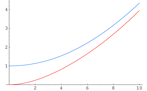 |
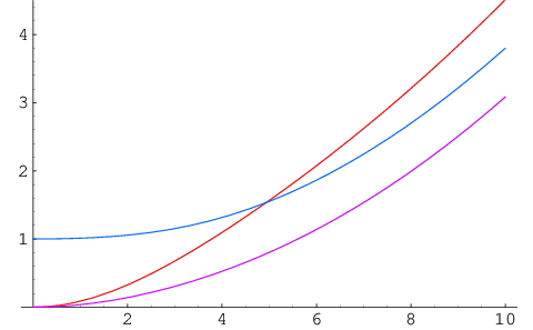
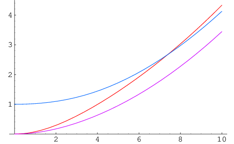
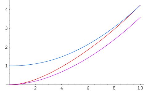
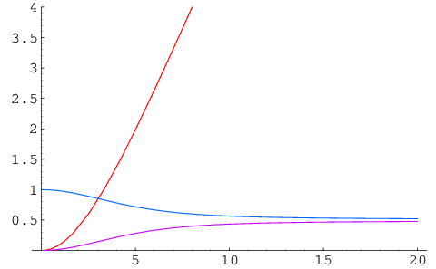
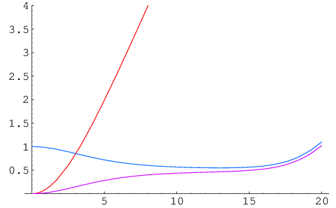
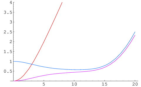
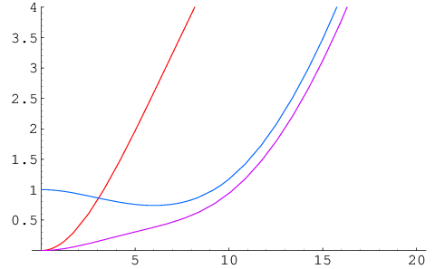
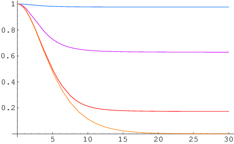
Here we present some plots of the numerical solutions to illustrate the qualitative behaviour of the metric functions for various values of .
In Figure 2 we show plots of the functions for large values of . We see that in the IR the behaviour is that of the space . However, despite starting below (at zero), the function eventually crosses , in agreement with the UV expansions. The crossing point moves further and further along the radial direction as is increased. In Figure 3 we plot the functions for values of close to the minimum.
 |
 |
 |
 |
We see that in the IR the functions are all very close to the special case . However, when is not exactly equal to its minimum value, the functions start to deviate at some point. For values of closer and closer to the special one, there is a larger and larger region where the functions are well approximated by the profiles of the Maldacena-Nastase solution.
 |
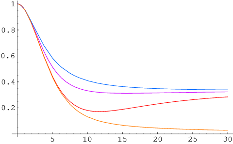 |
Finally, in Figure 4, we plotted the dilaton and the function for various values of the constant . We see that the generically goes to a constant at infinity, while in the particular case of Maldacena-Nastase vanishes in the UV.
3.4 Limits
In this subsection we analyse two special limits of the one-parameter solutions, namely and , respectively.
The solution for holonomy with flux
The numerical solutions show that by increasing the value of the solution looks more and more like the manifold . To see this more precisely, we will consider an expansion of the functions and in inverse powers1111 11 From (3.29) it can be checked a posteriori that the first few terms reproduce the UV expansions (3.22). Therefore the series (3.28) is certainly not valid for . In any case, we only need this for large here. of of the form:
| (3.28) | ||||
For small it can be checked that this agrees with the IR expansions (3.20). Then one can solve the system (3.7) order by order in powers of . There are of course different solutions depending on the boundary conditions and here we will concentrate on the boundary conditions already treated in Section 3.3. For our purpose, we only need the first few orders of the expansion (3.28). These read
| (3.29) | ||||
where is a function of the radial coordinate defined as in Section 2.2, namely
| (3.30) |
The functions at the lowest order in the expansion solve a simplified version of (3.7) where , which are simply the differential equations for the holonomy metric . The metric in terms of the expansion (3.28) reads
| (3.31) |
thus, at leading order in , the solution looks like the manifold with a very large , and units of flux through it. One could of course take while keeping fixed, by taking at the same time. This is an exact solution, where the flux vanishes.
The solution for : holonomy with branes
Here we show that when is very close to the minimum value , there is a region where the solution looks like a holonomy manifold with fivebranes wrapped on the non-trivial three-sphere. The calculation is analogous to that appearing in Section A.2 of [14].
The solution stays close to the Maldacena-Nastase solution up to large values of . To analyse the behaviour of the solution where it starts departing from this, we consider the following ansatz for an approximate solution
| (3.32) | ||||||
The leading terms are those of the Maldacena-Nastase solution and we require that , . Anticipating the form of the metric that we are after, we change coordinates as follows
| (3.33) |
We could also have taken in front, but since we will find that , this does not matter. Then we plug the ansatz (3.32) into the BPS equations (3.7) and expand to first order in the . The equation for is satisfied automatically at leading order. Working at large , we can solve the equations for and we find
| (3.34) | ||||
where are two integration constants. We can determine the dilaton with the same precision by considering the ansatz
| (3.35) |
where . Then we find
| (3.36) |
where is another integration constant. Inserting these back into the metric and changing coordinates as we find
| (3.37) | ||||
This is the approximate solution for fivebranes in flat space, wrapped on the three-sphere parameterised by . More precisely, we see that the topology is that of , where the three-sphere transverse to the branes (defined by ) vanishes smoothly. Hence this is the same topology of the holonomy manifold . The fivebranes then can be wrapping or .
This approximation however requires that is large, but at the same time , where is defined by . Presumably around the solution looks more accurately like [14], but this seems difficult to analyse in the linearised approximation. We can also estimate the relation between and by extrapolating to zero the value of . This gives
| (3.38) |
3.5 Summary
In this section we have discussed a set of gravity solutions characterised by a non-trivial parameter . The additional parameters of the solutions are the integral units of NS three-form flux and the asymptotic value of the dilaton . The constant is a function of and , that may be determined numerically. There are six different solutions, exchanged by the action of the triality group . In each case the internal seven-dimensional manifold is an asymptotically conical space, with topology , that we have denoted , with . The base of the asymptotic cone is the nearly Kähler manifold with metric [25]. More precisely, the topology of the space is that of the holonomy manifold , that we reviewed in Section 2.
In each case the parameter gives the size of the non-trivial at the origin, hence this is analogous to the deformation in the deformed conifold. On the other hand, one can also define a resolution parameter by looking at how the metric breaks a symmetry at large distances. In particular, we have argued that the parameter gives a measure of how much the space deviates from the geometry. Hence, from this point of view, can be interpreted as an effective resolution parameter. In the case of holonomy the moduli space of metrics on has three different branches, meeting at the origin. With an abuse of language1212 12 In particular, we do not use these words here in the sense of complex or symplectic geometry., we can say that the singular cone over may be deformed, resolved or flopped-resolved, with the three possibilities mutually exclusive. The six solutions that we discussed may be said to be deformed and resolved, analogously to the resolved deformed conifold geometry [11, 14].
When is very large the solution approaches a holonomy manifold with flux on a large three-sphere. When hits the lower bound , the geometry becomes a solution of the type discussed by [23], corresponding to the near-brane limit of a large number of fivebranes wrapped on the inside a manifold with topology . These have a finite size three-sphere at the origin, but are asymptotically linear dilaton backgrounds. When is very close to the critical value the solution stays close to the near-brane Maldacena-Nastase one up to large values of (see the plots in Figure 3) and when it starts deviating from this behaviour the geometry becomes approximately that of the manifold with fivebranes wrapping the non-trivial three-sphere inside this.
 |
 |
For each solution the parameter interpolates between the holonomy manifold with units of flux on a large three-sphere, and the holonomy manifold with fivebranes wrapped on a (different) three-sphere. Hence, this may be interpreted as a realisation of a geometric transition, purely in the context of supergravity. Notice that this is different from the closely related setup in [26, 25], where the relevant geometric transition involved D6 branes wrapped in the conifold, although this was embedded in the holonomy context by uplifting to M-theory.
From the point of view of the holonomy manifold (say) with units of flux through the three-sphere , the two solutions and break the symmetry under in two opposite directions. These look like a “resolution” of the manifold and its flopped version. The breaking of this symmetry is analogous to the breaking of the symmetry in the resolved deformed conifold. On the other hand, from the point of view of the branes wrapped on the three-sphere in , the two solutions and break the symmetry generated by by “deforming” the original manifold in two different ways. In other words, the geometric transition may proceed from branes in to flux in or from branes in to flux in . There is no analogue of this in the conifold case.
Moreover, depending on which three-sphere of the branes wrap, in the geometry after the backreaction this three-sphere may become contractible or not. For example, if the fivebranes were wrapped on and after the geometric transition we have the manifold (with flux), the sphere wrapped by the branes is contractible. Whereas if the fivebranes were wrapped on and after the geometric transition we have the manifold (with flux), the sphere wrapped by the branes is not contractible. This phenomenon has no analogue in the conifold case, where the two-sphere wrapped by the branes always becomes contractible in the backreacted geometry. In the context of the discussion in [23] these two possibilities led to two different values of the quantity denoted , defined as the flux of through the three-sphere wrapped by the branes. In particular, for the basic solution of [23] (with topology) it was assumed that the three-sphere wrapped by the branes is and therefore . The second solution of [23] (with topology) was interpreted as arising from fivebranes still wrapped on and therefore here . Cf. Table 1. This ambiguity may also be understood as related to different gauge choices for the connection on the normal bundle to the wrapped three-sphere. In [23] it was explained how this corresponds to changing the number of fermionic zero modes on the brane worldvolume with all choices leading to equivalent results for the physical Chern-Simons level of the dual gauge theory, namely .
4 Type IIA solutions with interpolating structures
In this section we will discuss solutions of Type IIA supergravity of the type , where the internal seven-dimensional manifold has a structure and there are various fluxes. We will then show that starting from a torsional geometry one can obtain a more general solution, interpolating between the original solution and a warped holonomy solution. The method that we use is quite general and can be applied to supergravity solutions different from the ones of the previous section.
4.1 Supersymmetry conditions
We write the metric ansatz in string frame as
| (4.1) |
The solutions are characterised by a structure on the internal space, namely an associative three-form (and its Hodge dual) and a non-trivial phase . The non-zero fluxes are the RR four-form and the NS three-form . The equations characterising the geometry may be written in the form of generalised calibration conditions [34], and can be obtained straightforwardly by reducing the equations presented in [35] from eleven to ten dimensions. Some details of this reduction are presented in Appendix C. The equations read
| (4.2) | ||||
In addition, the fluxes are determined as follows
| (4.3) | ||||
Notice the relation
| (4.4) |
From the results of [35] we have that any solution to these conditions, supplemented by the Bianchi identities , solves also the equations of motion. This geometry is the analogue of the interpolating structure geometry discussed in [29, 30]. Notice that this case is not contained in the equations presented in [36], which instead describe an structure in seven dimensions. Although the ansatz for the bosonic fields in the latter reference is equivalent to ours, the ansatz for the Killing spinors does not allow the structure that we are discussing here. The interested reader can find a discussion of spinor ansatze in Appendix C.
The conditions (4.2), (4.3) include the Type I torsional geometries as a special case, which are obtained simply setting . The warp factor is related1313 13 An integration constant can always be reabsorbed in a scaling of the coordinates. to the dilaton as so that the ten-dimensional metric in string frame is unwarped. The limit is slightly singular, since in this case the structure in eleven dimensions from which our equations have been obtained breaks down1414 14 In particular, the one-form does not exist. See Appendix C and [35].. However, going back to the equations in [35], one can see that in this limit the internal eight-dimensional geometry becomes a warped Spin(7) manifold with self-dual flux [37]. A careful analysis then shows that in the limit we obtain the warped holonomy solutions derived in [31]. The warp factor is again related to the dilaton
| (4.5) |
and rescaling the internal metric as the full metric becomes
| (4.6) |
where the rescaled metric now has holonomy, namely . Taking directly the limit on the relation (4.4) gives . Hence the four-form flux can be written as
| (4.7) |
The equation of motion for implies that the warp factor is harmonic with respect to the metric, namely
| (4.8) |
4.2 Solution generating method
We now discuss two different methods to generate solutions of the equations presented above, starting from a solution of the Type I torsional system. One method, analogous to the procedure discussed in [14], involves a simple chain of dualities. Another method exploits the form of the supersymmetry conditions. We will refer to this second method as “rotation” [29, 30].
Dualities
We start with a solution of (3.2). The non-trivial fields are the dilaton , the three-form flux and the metric . First we uplift to eleven dimensions. We rescale the new eleventh dimension by a constant factor , boost along with parameter , and finally undo the rescaling of . This gives the transformation
| (4.9) |
Then we reduce back to Type IIA along the transformed and we perform two T-dualities along the two spatial directions of the part. At the level of brane charges, the steps in the transformation may be summarised as
NS5 M5 M5, NS5, D0 NS5, D2
Notice that a non-zero magnetic field will be generated in the process. The dualities above result in the following Type IIA solution
| (4.10) | ||||
where here the hatted quantities denote the new solution while the unhatted ones denote the initial solution. Notice that in contrast to the case in [14] the dilaton is changed in the transformation. This can be understood because here the procedure introduces D2 branes, to which the dilaton couples. Notice also that we need , which imposes . Thus the transformation may be applied only if in the initial solution the dilaton is a bounded function. We can write the transformed fluxes as
| (4.11) | ||||
from which we can read off the internal field in terms of the associative three-form , namely
| (4.12) |
From these expressions it is clear that the Bianchi identities of the initial solution imply the ones of the transformed solution. In principle this method may be applied also to non-supersymmetric solutions.
Rotation
The same transformation can be done directly on the supersymmetry equations, without doing any dualities. One advantage of this method is for example that it is applicable to configurations with sources [30]. Suppose that and a three-form are a solution of the system (3.2). Then one can define
| (4.13) | ||||
and a new seven-dimensional metric . It is easy to check that the new quantities , and are a solution of the first three equations of the general system (4.2). The fourth one can be solved and it gives a relation between and the dilaton of the original solution:
| (4.14) |
Here and are integration constants. The rotated background in terms of unrotated quantities reads
| (4.15) | ||||
In order to match the result of this method to the previous one, one has to identify
| (4.16) |
As before, the Bianchi identities of the general solution follow immediately from the ones of the unrotated solution.
4.3 Deformations of the warped holonomy solutions
We can now apply the transformation above to the solutions of Section 3. Notice that indeed in those solutions the dilaton was bounded from below. For each solution of Section 3 we then obtain a one-parameter family of solutions of Type IIA supergravity, with D2 brane charge and an internal field. The background is simply obtained by plugging the solutions of Section 3 into the equations (4.10) or (4.15). Notice that the warp factor in (4.10) goes to one at infinity. However, for AdS/CFT applications, one would like to take a decoupling limit in which the warp factor goes to zero at infinity. In this way the asymptotically Minkowski region is removed and replaced by a boundary. We will be more precise about the asymptotics momentarily. To proceed, first recall that one should quantise the transformed three-form as
| (4.17) |
where is the appropriate non-trivial three-sphere in each case. Then rescaling the Minkowski coordinates as
| (4.18) |
in the limit , keeping fixed, the metric is finite and reads
| (4.19) |
Here does not have a factor of and the new warp factor goes to zero at infinity. The factor of makes sure that the asymptotic form of the metric is independent of and in addition will allow us to take the further limit . From the expressions in (4.10) we see that this limit is problematic for the transformed and dilaton . To obtain a finite limit we also send , while keeping fixed
| (4.20) |
The factor on the right-hand side is again inserted to allow to take a further limit in the solution. Now taking the solution is then completed with1515 15 In the expressions below enters only in the combination , which is finite in the limit.
| (4.21) | ||||
Here tildes on and indicate that the expressions are computed with the metric . We can now show that in this solution the limit gives a solution of the type found in [31]. Firstly, as we saw in Section 3.4, for large the metric for each solution reads
| (4.22) |
From the differential equation for the dilaton we find that
| (4.23) |
where is the warp factor of the solution found in [31], which reads
| (4.24) | ||||
is an integration constant and taking we have that when . Solving for the dilaton in an expansion in we find
| (4.25) |
Notice that although this was obtained in [31] for the holonomy metric on , it follows from our discussion in Section 3.4, that this expression is invariant under and hence the same function in (4.24) appears for any . Thus taking the limit on a solution, gives the following solution
| (4.26) | ||||
where is a harmonic three-form1616 16 This can be extracted from the limit of . on . This is precisely the warped solution presented in [31]. Notice that asymptotically the string frame metric goes to AdS, where , however the dilaton vanishes like . In fact, by setting we have the exact solution with metric
| (4.27) |
and non-trivial and fluxes. However, the solution does not have conformal symmetry because the dilaton depends on the radial coordinate . In (4.27) we can replace with another nearly Kähler metric, provided there exists the appropriate harmonic three-form on the cone, thus obtaining a solution generically preserving the same amount of supersymmetry. These metrics are in fact solutions of massive Type IIA supergravity [38]. This is a curious fact that might be relevant for AdS/CFT applications [39].
In conclusion, for any solution of the type of [31], arising from configurations of D2 branes and fractional NS5 branes transverse to a manifold , we have constructed a one-parameter family of deformations, with the same AdS asymptotics. These are analogous to the baryonic branch deformations [11] of the Klebanov-Strassler solution [8]. In particular, they break the symmetry of a holonomy manifold .
5 Discussion
In this paper we have discussed various supergravity solutions related to configurations of fivebranes wrapping a three-sphere in a holonomy manifold . Our basic solutions are examples of torsional manifolds [27] and comprise some cases previously studied in [33, 23, 22]. There are six solutions characterised by a non-trivial parameter. As we change this parameter, each solution interpolates between a manifold with (NS5 or D5) branes on a three-sphere and a distinct manifold with (NS or RR) flux on a different three-sphere. This is then an explicit realisation of a geometric transition between a pair of manifolds, analogous to the version of the conifold transition described in [14]. The six solutions pairwise connect the three branches of the classical moduli space of holonomy metrics on [25]. It would be interesting to see if the picture that we discussed, which is purely classical, may be related to a “large duality” similar to [16].
From each of the basic solutions we constructed new Type IIA backgrounds with D2 brane charge by employing a simple generating method applicable to a class of geometries with interpolating structure. The solutions constructed in this way are one-parameter deformations of the solutions presented in [31], corresponding to D2 branes and fractional NS5 branes transverse to the manifold . Therefore, they are analogous to the baryonic branch deformation [11] of the Klebanov-Strassler solution [8].
Based purely on supergravity considerations, it is natural to expect a close relation between the Chern-Simons theory discussed in [23] and the three-dimensional field theory dual to the solutions above. Let us conclude with some speculations about the field theory duals. First of all, the existence of a finite size in the geometry suggests that the IR field theory should be confining, as in [23]. A standard computation of the number of D2 branes shows that this is running, and vanishes in the IR, as1717 17 Here the running is not logarithmic, but we have at large . the number of D3 branes in [8]. This suggests that the three-dimensional field theory may be a quiver with gauge group . Moreover, we expect that the three-form flux will induce Chern-Simons terms, like in [23]. We also have a running field on a three-sphere at infinity, analogous to the field in [8], with , suggesting the relation . A possible scenario is therefore that the solution of [31] describes a “cascading” three-dimensional quiver, which in the “last step” becomes the theory of [23]. However, an important caveat is that our solutions are related to NS5 branes in Type IIA, while the discussion in [23] applies to configurations of Type IIB NS5 branes. Nevertheless, the relation between the various solutions based on the conifold and the solutions we discussed here indicates that a precise connection between the four-dimensional “parent” field theories and the three-dimensional field theories should exist, along the lines of [40, 41]. In particular, we can uplift our solutions to M-theory and subsequently reduce along a inside the non-trivial geometry, thus obtaining solutions with the topology of the deformed or resolved conifold [26] (times ).
Another relationship between the Chern-Simons theory and the putative field theory dual to [31] is suggested by the one-parameter deformations of [31] that we described. In particular, we saw how in a certain regime of the parameter () the solution becomes close to the fivebrane geometry. The presence of a large field on the three-sphere wrapped by these branes suggests that perhaps the relevant field theory is the theory on fivebranes wrapped on a fuzzy three-sphere [14].
We leave the investigation of these ideas for future work.
Acknowledgements
We are very grateful to Juan Maldacena, Carlos Núñez, Johannes Schmude and James Sparks for discussions and useful comments. We also thank Diego Rodriguez-Gomez for comments and collaboration on related topics. D. M. is partially supported by an EPSRC Advanced Fellowship EP/D07150X/3.
Appendix A invariant one-forms
Consider three elements obeying the constraint . We define the following Lie-algebra valued one-forms
| (A.1) | ||||
where are Pauli matrices. We can invert these obtaining
| (A.2) | ||||
Parameterising the group elements explicitly in terms of angular variables as
| (A.3) | ||||
after some computation we get
| (A.4) | ||||
Notice and are left-invariant one-forms, obeying
| (A.5) |
and cyclic permutations. We can also define the following Lie-algebra valued one-forms
| (A.6) | ||||
A similar computation gives
| (A.7) | ||||
These are right-invariant one-forms, obeying
| (A.8) |
and cyclic permutations. Computing the we obtain
| (A.9) |
where is the following matrix
| (A.10) |
We note the following identities
| (A.11) |
and
| (A.12) |
To prove the latter we have to use and . We identify the above with the (left-invariant) one-forms and used in the main text
| (A.13) | ||||
where the minus signs have been included in order to match with our conventions on the Lie-algebra relations , etcetera. Notice that
| (A.14) |
We also define
| (A.15) | ||||
Appendix B Derivation of the BPS equations
In the following we derive the BPS system (3.7) from the structure equations (3.2). Recall the metric ansatz is
| (B.1) |
In this section we define the orthonormal frame with an extra factor of with respect to the definition (2.14), namely here
| (B.2) |
so that the associative three form in the following is defined as
| (B.3) |
and we use the definitions in (2.16). Let us look at the first equation in (3.2). We first compute some useful intermediate results:
| (B.4) | |||||
| (B.5) | |||||
| (B.6) | |||||
| (B.7) | |||||
where we used the identity
| (B.8) |
After some more algebra we find
| (B.9) | |||||
Thus the first equation in (3.2) implies
| (B.10) |
Let us now look at the second equation in (3.2). We first calculate
| (B.11) | |||||
The equation may be written as
| (B.12) |
and after writing , it may be regarded as giving the derivative of the dilaton in terms of the remaining functions. In particular
| (B.13) |
Finally we analyse the last equation in (3.2). This can be rewritten as
| (B.14) |
Then we compute :
| (B.15) | |||||
We now need to compute . First, starting from the ansatz (3.4) and using the relations (3.17) we obtain:
| (B.16) | |||||
Then the Hodge dual is:
| (B.17) | |||||
Putting everything together we find:
| (B.18) | ||||
where the angle is fixed in terms of the other functions and reads:
| (B.19) |
Finally, substituting the functions , and with the functions , and using a computer program to simplify the expressions, we find the BPS system (3.7).
Appendix C Supersymmetry conditions in Type IIA
C.1 Reduction from
General conditions characterising solutions of eleven-dimensional supergravity of the warped product type where is either or AdS3, were presented in [35]. Here we are interested in the case that . The eleven-dimensional metric is written as
| (C.1) |
and the four-form flux reads
| (C.2) |
Thus is a four-form and is a one-form. Upon setting , the equations (3.11) - (3.16) of [35] become
| (C.3) | ||||
Here is a three-form, is a one-form and is a function, defined as spinor bilinears, that characterise the structure in eight dimensions. The seven-dimensional Hodge star operator is defined as and . The electric and magnetic fluxes are the determined in terms of the structure as
| (C.4) | ||||
The latter equation obeyed by the magnetic flux may be inverted giving
| (C.5) |
The one-form in general does not correspond to a Killing vector. However, in order to reduce to Type IIA, we will assume that the dual vector is Killing. In particular, writing , the eleven-dimensional metric takes the form
| (C.6) |
and its reduction to ten dimensions then can be simply read off:
| (C.7) |
Then we write
| (C.8) |
Looking first at the fluxes we find
| (C.9) | ||||
Using these equations, from (C.3) we obtain
| (C.10) | ||||
Finally, the reduction of the four-form gives the NS three-form and the RR four-form :
| (C.11) | ||||
C.2 Killing spinor ansatze
In this Appendix we discuss ansatze for the Killing spinors in eleven and ten dimensions. Although in the main text we have not derived the equations from the Killing spinors directly, it may be useful to spell out some details about spinors and representations of gamma matrices. The general spinor ansatz in eleven dimensions reads [35]
| (C.12) |
We use the following explicit representation of gamma matrices
| (C.13) | ||||
The are gamma-matrices and is the chirality matrix in , with . The denote gamma-matrices in . In an explicit representation these may be taken [35] as follows
| (C.14) |
where are Pauli matrices. The Majorana condition in eleven dimensions , with implies that and . Hence is a Majorana spinor in and are Majorana-Weyl spinors in .
To make the reduction to ten dimensions it is convenient to chose the following representation of gamma-matrices:
| (C.15) |
These are real and symmetric, taking to be purely imaginary and anti-symmetric. Then the chirality matrix is
| (C.16) |
and is again real and symmetric. We then write the Majorana-Weyl spinors as
| (C.17) |
where are two-component spinors and are eight-component spinors, which can all be taken to be real. Imposing the chirality conditions then implies
| (C.18) |
Thus, up to an overall real function, we can take
| (C.19) |
Upon reducing to Type IIA, the complexified Killing spinor is simply related to the Killing spinor in eleven dimension as , hence the ansatz may be written as
| (C.20) |
The ten-dimensional gamma matrices are the same as the eleven-dimensional ones up to a warp factor, where the eleventh one becomes the ten-dimensional chirality matrix. Namely
| (C.21) | ||||
and the ten-dimensional chirality matrix is
| (C.22) |
where we have used the convention that1818 18 Taking gives .
| (C.23) |
The Majorana condition on the complexified ten-dimensional spinor is , where we can take . Therefore we have
| (C.24) | ||||
which can be solved for example taking
| (C.25) |
The ten-dimensional chirality conditions give
| (C.26) | ||||
Therefore, up to overall factors (not necessarily constant) that we can reabsorb in , we can take
| (C.27) |
Comparing (C.12) with (C.20) we find
| (C.28) | ||||
Now using
| (C.29) | ||||
from [35], we compute
| (C.30) | ||||
Since we are interested in a strict structure, we must have . In fact, if and were not parallel, we could construct a vector , reducing the structure to . Then we have that
where we normalised the spinor as and . In conclusion, we have shown that the ten-dimensional Killing spinor takes the form
| (C.31) |
Note that this possibility is excluded in the spinor ansatz in [36]. See e.g. equation (A.3) of this reference.
References
- [1] J. M. Maldacena, “The large N limit of superconformal field theories and supergravity,” Adv. Theor. Math. Phys. 2, 231 (1998) [Int. J. Theor. Phys. 38, 1113 (1999)] [arXiv:hep-th/9711200].
- [2] A. Kehagias, “New type IIB vacua and their F-theory interpretation,” Phys. Lett. B 435, 337 (1998) [arXiv:hep-th/9805131].
- [3] I. R. Klebanov and E. Witten, “Superconformal field theory on threebranes at a Calabi-Yau singularity,” Nucl. Phys. B 536, 199 (1998) [arXiv:hep-th/9807080].
- [4] B. S. Acharya, J. M. Figueroa-O’Farrill, C. M. Hull and B. J. Spence, “Branes at conical singularities and holography,” Adv. Theor. Math. Phys. 2, 1249 (1999) [arXiv:hep-th/9808014].
- [5] D. R. Morrison and M. R. Plesser, “Non-spherical horizons. I,” Adv. Theor. Math. Phys. 3, 1 (1999) [arXiv:hep-th/9810201].
- [6] P. Candelas and X. C. de la Ossa, “Comments on Conifolds,” Nucl. Phys. B 342, 246 (1990).
- [7] A. Strominger, “Massless black holes and conifolds in string theory,” Nucl. Phys. B 451, 96 (1995) [arXiv:hep-th/9504090].
- [8] I. R. Klebanov and M. J. Strassler, “Supergravity and a confining gauge theory: Duality cascades and -resolution of naked singularities,” JHEP 0008, 052 (2000) [arXiv:hep-th/0007191].
- [9] J. M. Maldacena and C. Nunez, “Towards the large N limit of pure N = 1 super Yang Mills,” Phys. Rev. Lett. 86, 588 (2001) [arXiv:hep-th/0008001].
- [10] A. H. Chamseddine and M. S. Volkov, “Non-Abelian solitons in N = 4 gauged supergravity and leading order string theory,” Phys. Rev. D 57, 6242 (1998) [arXiv:hep-th/9711181].
- [11] A. Butti, M. Grana, R. Minasian, M. Petrini and A. Zaffaroni, “The baryonic branch of Klebanov-Strassler solution: A supersymmetric family of SU(3) structure backgrounds,” JHEP 0503, 069 (2005) [arXiv:hep-th/0412187].
- [12] S. S. Gubser, C. P. Herzog and I. R. Klebanov, “Symmetry breaking and axionic strings in the warped deformed conifold,” JHEP 0409, 036 (2004) [arXiv:hep-th/0405282].
- [13] A. Dymarsky, I. R. Klebanov and N. Seiberg, “On the moduli space of the cascading SU(M+p) x SU(p) gauge theory,” JHEP 0601, 155 (2006) [arXiv:hep-th/0511254].
- [14] J. Maldacena and D. Martelli, “The unwarped, resolved, deformed conifold: fivebranes and the baryonic branch of the Klebanov-Strassler theory,” JHEP 1001, 104 (2010) [arXiv:0906.0591 [hep-th]].
- [15] R. Casero, C. Nunez and A. Paredes, “Towards the string dual of N = 1 SQCD-like theories,” Phys. Rev. D 73, 086005 (2006) [arXiv:hep-th/0602027].
- [16] C. Vafa, “Superstrings and topological strings at large N,” J. Math. Phys. 42, 2798 (2001) [arXiv:hep-th/0008142].
- [17] A. Strominger, “Superstrings with Torsion,” Nucl. Phys. B 274, 253 (1986).
- [18] C. M. Hull, “Compactifications of the Heterotic Superstring,” Phys. Lett. B 178, 357 (1986).
- [19] N. Halmagyi, “Missing Mirrors: Type IIA Supergravity on the Resolved Conifold,” arXiv:1003.2121 [hep-th]. F. Chen, K. Dasgupta, P. Franche, S. Katz and R. Tatar, “Supersymmetric Configurations, Geometric Transitions and New Non-Kahler Manifolds,” arXiv:1007.5316 [hep-th].
- [20] R. Bryand and S. Salamon, “On the construction of some complete metrics with exceptional holonomy,” Duke Math. J. 58, 829 (1989).
- [21] G. W. Gibbons, D. N. Page and C. N. Pope, “Einstein Metrics on , and Bundles,” Commun. Math. Phys. 127, 529 (1990).
- [22] F. Canoura, P. Merlatti and A. V. Ramallo, “The supergravity dual of 3d supersymmetric gauge theories with unquenched flavors,” JHEP 0805, 011 (2008) [arXiv:0803.1475 [hep-th]].
- [23] J. M. Maldacena and H. S. Nastase, “The supergravity dual of a theory with dynamical supersymmetry breaking,” JHEP 0109, 024 (2001) [arXiv:hep-th/0105049].
- [24] A. H. Chamseddine and M. S. Volkov, “Non-Abelian vacua in D = 5, N = 4 gauged supergravity,” JHEP 0104, 023 (2001) [arXiv:hep-th/0101202].
- [25] M. Atiyah and E. Witten, “M-theory dynamics on a manifold of holonomy,” Adv. Theor. Math. Phys. 6, 1 (2003) [arXiv:hep-th/0107177].
- [26] M. Atiyah, J. M. Maldacena and C. Vafa, “An M-theory flop as a large N duality,” J. Math. Phys. 42, 3209 (2001) [arXiv:hep-th/0011256].
- [27] J. P. Gauntlett, D. Martelli, S. Pakis and D. Waldram, “-structures and wrapped NS5-branes,” Commun. Math. Phys. 247, 421 (2004) [arXiv:hep-th/0205050].
- [28] T. Friedrich and S. Ivanov, “Killing spinor equations in dimension 7 and geometry of integrable -manifolds,” arXiv:math/0112201.
- [29] R. Minasian, M. Petrini and A. Zaffaroni, “New families of interpolating type IIB backgrounds,” JHEP 1004, 080 (2010) [arXiv:0907.5147 [hep-th]].
- [30] J. Gaillard, D. Martelli, C. Nunez and I. Papadimitriou, “The warped, resolved, deformed conifold gets flavoured,” Nucl. Phys. B 843, 1 (2011) [arXiv:1004.4638 [hep-th]].
- [31] M. Cvetic, H. Lu and C. N. Pope, “Brane resolution through transgression,” Nucl. Phys. B 600, 103 (2001) [arXiv:hep-th/0011023].
- [32] M. Cvetic, G. W. Gibbons, H. Lu and C. N. Pope, “Supersymmetric M3-branes and Manifolds,” Nucl. Phys. B 620 (2002) 3 [arXiv:hep-th/0106026].
- [33] B. S. Acharya, J. P. Gauntlett and N. Kim, “Fivebranes wrapped on associative three-cycles,” Phys. Rev. D 63, 106003 (2001) [arXiv:hep-th/0011190].
- [34] J. Gutowski, G. Papadopoulos and P. K. Townsend, “Supersymmetry and generalized calibrations,” Phys. Rev. D 60, 106006 (1999) [arXiv:hep-th/9905156].
- [35] D. Martelli and J. Sparks, “-structures, fluxes and calibrations in M-theory,” Phys. Rev. D 68, 085014 (2003) [arXiv:hep-th/0306225].
- [36] M. Haack, D. Lust, L. Martucci and A. Tomasiello, “Domain walls from ten dimensions,” JHEP 0910, 089 (2009) [arXiv:0905.1582 [hep-th]].
- [37] K. Becker, “A note on compactifications on Spin(7)-holonomy manifolds,” JHEP 0105, 003 (2001) [arXiv:hep-th/0011114].
- [38] K. Behrndt and M. Cvetic, “General N = 1 Supersymmetric Flux Vacua of (Massive) Type IIA String Theory,” Phys. Rev. Lett. 95, 021601 (2005) [arXiv:hep-th/0403049].
- [39] D. Gaiotto and A. Tomasiello, “The gauge dual of Romans mass,” JHEP 1001, 015 (2010) [arXiv:0901.0969 [hep-th]].
- [40] M. Aganagic, “A Stringy Origin of M2 Brane Chern-Simons Theories,” Nucl. Phys. B 835, 1 (2010) [arXiv:0905.3415 [hep-th]].
- [41] D. Martelli and J. Sparks, “AdS4/CFT3 duals from M2-branes at hypersurface singularities and their deformations,” JHEP 0912, 017 (2009) [arXiv:0909.2036 [hep-th]].