Magnetic phases of spin-$\frac{3}{2}$ fermions on a spatially anisotropic square lattice

Extraordinary controllability of ultracold gases allows highly accurate modeling and study of problems originated in condensed matter physics. Frustrated magnetic systems occupy an important position on the list of intriguing problems that could be studied in multicomponent ultracold gases. Recently, multicomponent ultracold Fermi gases have attracted much attention [1, 2] motivated by the growing availability of hyperfine-degenerate fermionic atoms, such as ⁶Li, [3, 4, 5] ⁴⁰K, [6] ¹³⁵Ba and ¹³⁷Ba, [7] and ¹⁷³Yb. [8] Realization of unconventional phases of $SU(N)$ internally frustrated antiferromagnets[9] have been recently suggested[10, 11] in alkaline earth atoms with nuclear spin as large as $\frac{9}{2}$ in ⁸⁷Sr.

Among multicomponent ultracold gases, spin-$\frac{3}{2}$ alkaline fermions stand out by their rich physics characterized by an enlarged $Sp(4)$ symmetry, which is naturally present in the system without fine-tuning of any parameters. [12] By tuning the ratio of scattering lengths in the two allowed spin-$0$ and spin-$2$ channels, even the larger $SU(4)$ symmetry may be achieved.[12, 13, 14, 15]

Experiments with ultracold atoms are usually done in the presence of magnetic fields. For atoms with hyperfine spins $F\geq 1$, the spin-changing collisions redistribute the populations of the components with different spin projection $F^{z}$ while keeping the total magnetization $M=\sum_{j}F^{z}_{j}$ fixed. Therefore, the usual linear Zeeman effect induced by an external magnetic field does not play any role for a state with a fixed initially prepared $M$, and the main influence of an external magnetic field (except the change of scattering lengths due to the Feshbach resonance phenomenon) is contained in the quadratic Zeeman effect (QZE). The quadratic Zeeman field $q$ couples to $\sum_{j}(F_{j}^{z})^{2}$ and thus introduces a difference in chemical potentials for components with different $|F^{z}|$. A peculiar property of spin-$\frac{3}{2}$ fermions is the fact that even in presence of the quadratic Zeeman field, the high $Sp(4)$ symmetry is lowered to $SU(2)\times SU(2)$ and thus remains quite high. [16]

In this work, we study the magnetic phase diagram of spin-$\frac{3}{2}$ fermions at quarter filling, in the limit of a strong on-site repulsion, on an anisotropic square lattice with hopping amplitudes in two spatial directions differing by the factor $\lambda\in[0,1]$, as depicted in Fig. 1. We construct the effective field theory describing the low-energy properties of the system which has the form of a $Sp(N)$ extension of the $CP^{N-1}$ model, with the generically broken Lorentz invariance. For this field theory, the analysis of the one-loop renormalization group equations shows that the $Sp(N)$ terms are dangerously irrelevant: their presence leads to a considerable renormalization of the $CP^{N-1}$ part of the action. As the result, by changing the ratio of the scattering lengths or the lattice anisotropy parameter $\lambda$ one can drive the phase transition between the long range ordered Néel state and the valence-bond-solid (VBS) state.

We also include into consideration the quadratic Zeeman coupling and study the evolution of the ground state under QZE. Since the QZE preserves the $SU(2)$ symmetry,[16] the ground state at large values of the quadratic Zeeman field $q$ corresponds to the long-range ordered (Néel) phase of the isotropic spin-1/2 Heisenberg antiferromagnet (HAFM), for any nonzero value of the lattice anisotropy parameter $\lambda\neq 0$. We show that, depending on the value of the anisotropy $\lambda$, when the field $q$ is decreased, this state either adiabatically evolves into the Néel phase of 4-component fermions or undergoes a phase transition into the VBS state.

The structure of the paper is as follows: in Sect. II we present the derivation of the low-energy effective field theory for a system spin-$\frac{3}{2}$ fermions at quarter filling in the regime of a Mott insulator (in other words, in the regime of the $Sp(4)$ Heisenberg model). In Sect. III we analyze the renormalization group flow of the derived model and sketch the phase diagram of the system in dimensions one and two. In Sect. IV we study the effect of an external quadratic Zeeman field; finally, Sect. V contains the summary and discussion of the results.

Consider a system of spin-$\frac{3}{2}$ fermions on a two-dimensional anisotropic square lattice. In the $s$-wave scattering approximation, this system can be described by the following Hamiltonian: [12]

where $c_{\sigma,i}$ are the spin-$\frac{3}{2}$ fermionic operators at the lattice site $i$, $t_{ij}$ are the effective hopping amplitudes between two neighboring sites, $P_{Fm,i}=\sum_{\sigma\sigma^{\prime}}\langle Fm|\frac{3}{2}\sigma,\frac{3}{2}\sigma^{\prime}\rangle c_{\sigma,i}c_{\sigma^{\prime},i}$ are the operators describing an on-site pair with the total spin $F$, and the positive interaction constants $U_{0}$, $U_{2}$ are proportional to the scattering lengths in the $F=0$ and $F=2$ channels, respectively. The hopping is assumed to be generally anisotropic in two spatial directions, i.e.,

Although our main interest will be in the behavior of the two-dimensional model, we will also make a few comments about the one-dimensional case which formally corresponds to $\lambda=0$.

We will be also interested in the effect of the external magnetic field. Since the total magnetization in cold atom experiments has very long relaxation time, the primary effect of the external field is given by the quadratic Zeeman term:

At quarter filling (one particle per site), and in the limit of strong on-site repulsion $t_{ij}\ll U_{0},U_{2}$ the charge degrees of freedom are strongly gapped and the system can be approximately described by an effective spin Hamiltonian, which can be conveniently written in the following form:[12, 13, 14, 15]

where the $4\times 4$ matrices $\Gamma^{a}$ and $\Gamma^{ab}=\frac{1}{2i}[\Gamma^{a},\Gamma^{b}]$ are the generators of the $SU(4)$ Lie algebra. The operators $\widehat{\Gamma}^{a}$ form a vector representation of the $Sp(4)$ group, and $\widehat{\Gamma}^{ab}$ form an adjoint representation of $Sp(4)$, so the Hamiltonian (4) is explicitly $Sp(4)$-invariant.

In the second order of the perturbation theory in $t$, the exchange constants $J_{1,2}$ are given by:

The operators $\widehat{\Gamma}^{a}$, $\widehat{\Gamma}^{ab}$ can be expressed in terms of four Schwinger bosons $b_{\alpha}$, $1\leq\alpha\leq 4$, satisfying the constraint $b^{{\dagger}}_{\alpha}b_{\alpha}=1$ at each site: effectively one can just replace the operators $c_{\sigma,i}$ by $b_{\alpha,i}$ in the definition of $\widehat{\Gamma}$ in (4). Doing so, one arrives at the Hamiltonian of the form[17]

where $\mathcal{J}$ is the antisymmetric matrix that has the following properties:

One specific representation of the matrices introduced above is given by: [17]

where $\sigma^{a}$ are the Pauli matrices. The $Sp(4)$ group may be viewed as a group of unitary $4\times 4$ matrices $U$ that satisfy the condition $U^{T}\mathcal{J}U=\mathcal{J}$.

The couplings $J$, $J^{\prime}$ in (6) are given by:

and are assumed to be positive; in terms of the atomic spin-$\frac{3}{2}$ system this corresponds to the assumption

The Hamiltonian in the form (6) can be easily generalized to the case of an even number $N$ of bosonic flavors $b_{\alpha}$, $\alpha\in[1,N]$ and the local hardcore constraint for the Schwinger bosons is generalized by

with the number $n_{c}$ playing the role of the “spin magnitude”.[18]

The $Sp(N)$ symmetry of the Hamiltonian is enlarged to $SU(N)$ at the point $J=0$, where the two-site Hamiltonian becomes a permutation operator of two $N$-component objects. Since the lattice is bipartite, the enlargement of symmetry to $SU(N)$ happens also at $J^{\prime}=0$ point.[12, 13, 14, 15, 17] The latter point $J^{\prime}=0$ corresponds to a $SU(N)$ antiferromagnet where spins transform according to the fundamental representations of $SU(N)$ on sublattice A and according to the conjugate representation on sublattice B. In the following we will refer to this point as the staggered $SU(N)$ antiferromagnetic point. The other $SU(N)$ point $J=0$, where spins are in the fundamental representations of $SU(N)$ on each site, corresponds to the exactly solvable Uimin-Lai-Sutherland model in one dimension[19] and we will call it the uniform $SU(N)$ antiferromagnetic point.

Our strategy will be to use the staggered $SU(N)$ antiferromagnetic point $J^{\prime}=0$ (i.e., $U_{2}\to\infty$) as the starting point to construct the effective low-energy field theory. First of all, we make a unitary transformation[15, 17] on one sublattice,

that effectively interchanges the operators $\widehat{Q}$ and $\widehat{K}$ in the Hamiltonian (6). Further, we use the usual coherent state path integral formalism, passing from the bosonic operators $\widehat{b}_{\alpha,n}$ to the corresponding $c$-number lattice variables $\bm{b}_{n}$. It is easy to see that at the mean-field level both terms in the Hamiltonian (6) are simultaneously minimized for a uniform distribution of $\bm{b}_{n}$, provided that $J,J^{\prime}>0$. Thus, in the parameter region $J,J^{\prime}>0$ in (6) one may expect the physics to be rather different from that found in $Sp(N)$ models describing geometrically frustrated systems.[20]

In terms of $\bm{b}_{n}$, the Euclidean action on the lattice takes the form $\mathcal{A}_{\rm lat}=\int d\tau\mathcal{L}_{\rm lat}$, with the Lagrangian:

In a standard manner, we then split the field $\bm{b}$ into the smooth and staggered components $\bm{z}_{n}$, $\bm{\psi}_{n}$ :

where $\eta_{n}$ takes values of $\pm 1$ on $A$ and $B$ sublattices, respectively, and the constraints

are implied. One can expect that the magnitude of the staggered component $\bm{\psi}$ that corresponds to ferromagnetic fluctuations, will be much smaller than that of $\bm{z}$.

The unitary transformation (9) is a necessary step: for positive $J^{\prime}$ one cannot start from the uniform $SU(N)$ antiferromagnetic point $J=0$, since no reasonable choice of smooth fields is possible. It has to be remarked, however, that our choice of smooth fields becomes poor in the vicinity of the point $J=0$ that has a much higher degeneracy of the mean-field ground state. One may thus expect that the resulting effective field theory is not reliable close to the uniform $SU(N)$ antiferromagnetic point.

Passing to the continuum and making the gradient expansion, while retaining only up to quadratic terms in $\bm{\psi}$ and neglecting its derivatives, one readily obtains the Euclidean action in the form $\mathcal{A}=\mathcal{A}_{0}+\mathcal{A}_{\rm int}+\mathcal{A}_{\rm top}$, where $\mathcal{A}_{0}$ corresponds to $J^{\prime}=0$:

The term $\mathcal{A}_{\rm top}$ contains the topological phase contribution, [21, 22, 18]

and the perturbation $\mathcal{A}_{\rm int}$ is determined by the deviation $J^{\prime}$ from the staggered antiferromagnetic $SU(4)$ point:

Here and throughout the paper we use the notation

In the above expressions, $d=1$ or $2$ is the spatial dimension, the index $k=1,\ldots,d$ labels spatial coordinates, and the lattice constant $a$ and the Planck constant has been set to unity for convenience. The factor $\sqrt{\lambda}$ comes from rescaling one of the coordinates to compensate for the anisotropy of interactions (for $d=1$ one has to set effectively $\lambda=1$), and $\mu_{1,2}$ are the Lagrange multipliers ensuring the constraints.

Integrating out the staggered component $\bm{\psi}$ can be easily performed (see Appendix A for details), and one arrives at the following effective action for the complex unit vector field $\bm{z}$:

Here $\Lambda$ is the ultraviolet momentum cutoff, $x^{0}=2J\tau\sqrt{d-1+\lambda}$ is the rescaled imaginary time coordinate, $\mathcal{D}_{\mu}=\partial_{\mu}-i\mathcal{A}_{\mu}$ is the gauge covariant derivative, and $\mathcal{A}_{\mu}=-i(\bm{z}^{*}\cdot\partial_{\mu}\bm{z})$ is the gauge field. It is worth noting that $\widetilde{\bm{z}}\cdot\mathcal{D}_{\mu}\bm{z}\equiv\widetilde{\bm{z}}\cdot\partial_{\mu}\bm{z}$ since $\widetilde{\bm{z}}\cdot\bm{z}=0$. The bare values of the coupling constants in (17) are given by the following expressions:

In particular, note the different signs of $\widetilde{g_{1}}$ and $\widetilde{g_{2}}$. The first two terms in the action (17) constitute the familiar action of the $CP^{N-1}$ model,[23, 24, 25, 26, 27] that has been extensively studied as an effective theory for $SU(N)$ antiferromagnets [22, 18]. The third and fourth terms are proportional to $J^{\prime}$ and thus represent perturbation caused by the deviation from the $SU(N)$ staggered antiferromagnetic point. The presence of those terms has been noticed by Qi and Xu,[17] but they have been neglected since they seem to be irrelevant. In the next section, we will show that those $Sp(N)$ terms are generally only marginally irrelevant, and can drive a phase transition.

Here a remark is in order: in the action above, for the 2d case we have effectively removed the lattice anisotropy by rescaling one of the coordinates. Due to the $Sp(4)$ symmetry of the problem, the remaining perturbations that break the 90 degree rotation symmetry of the lattice appear only in higher orders in field derivatives: the lowest-order terms of this type have the form $f_{\mu}|\bm{z}^{*}\mathcal{D}^{2}_{\mu}\bm{z}|^{2}$ and $f_{\mu}(\widetilde{\bm{z}}\mathcal{D}_{\mu}\bm{z})(\widetilde{\bm{z}}^{*}D^{2}_{\mu}\bm{z}^{*})+\text{c.c.}$, with $f_{x}\not=f_{y}$. Such terms are less relevant than those taken into account in the action (17) and thus will be neglected.

The properties of the $CP^{N-1}$ model are well understood: in the absence of the topological term $\mathcal{A}_{\rm top}$ given by (14), it is always disordered in $d=1$, and in $d=2$ the long range order appears below a certain critical value of the effective coupling.[25, 26] This critical value depends on $N$, and from the numerical work [28, 29, 30] it is known that the two-dimensional $CP^{N-1}$ model on a square lattice is disordered for $N/n_{c}\geq 5$.

In the disordered phase the field $\bm{z}$ acquires a finite mass, and a kinetic term for the gauge field is dynamically generated. [26] It is also well known that the topological term becomes crucially important in the disordered phase; [21, 22, 18] particularly, it leads to a spontaneous dimerization in $d=1$ for odd $n_{c}$ (except for $N=2$ which is special: in that case the system remains gapless and translationally invariant in a wide $g$ range[31, 32, 33, 34]), and in $d=2$ the disordered phase gets spontaneously dimerized in different patterns depending on the value of $(n_{c}\mod 4)$. The “disordered” phase thus acquires valence bond solid (VBS) order connected to the broken translational invariance. For the $Sp(4)$ case, parent Hamiltonians with exact ground states of the VBS type have been constructed recently.[35]

An effective theory for the $Sp(N)$ Heisenberg model in a form similar to (17) has been obtained by Kataoka et al.[36] However, our result differs from that of Ref. 36 in one important respect: the last two terms in (17), proportional to the “perturbation” $J^{\prime}$, explicitly break the Lorentz invariance, while in the theory of Ref. 36 the Lorentz invariance is retained even in the presence of the “perturbation”. By a simple classical linear excitation analysis of the initial lattice action (10) one can obtain $(N-1)$ Goldstone modes (“spin waves”), having the velocities $v_{1}=v_{2}=\ldots=v_{N-2}=1$ and $v_{N-1}=1+J^{\prime}/J$ (in units of $2J\sqrt{d}$), see Appendix B for details. Our effective theory (17) yields $(N-2)$ modes with the velocity $u_{1}=\sqrt{\gamma}$ and one mode with the velocity $u_{2}=u_{1}\sqrt{(1+\rho)/(1-\kappa)}$, where $\gamma=g_{1}/g_{2}$, $\rho=g_{2}/\widetilde{g_{2}}$, and $\kappa=-g_{1}/\widetilde{g_{1}}$. After substituting the bare values of Eq. (18), this is in a perfect agreement with the spin wave calculation, while the theory of Ref. 36 yields the same velocity $v=1$ for all three modes.

For $N=4$, the contribution of the quadratic Zeeman field (3) takes the following form:

with the bare “mass” value given by

For any finite $q$, the symmetry of the model is reduced from $Sp(4)$ to $SU(2)\times SU(2)$[16]. If $q$ is large enough, the effective theory reduces to that of a two-component complex field, i.e., to the $CP^{1}$ model.

Consider first the case when the external field is absent. To understand the role of the $Sp(N)$ terms in the action (17), we have to analyze their behavior under renormalization. Renormalization group (RG) equations for spin liquids described by a Lorentz-invariant low-energy field theory with $SU(N)$ and $Sp(N)$ symmetries have been studied recently[37] by means of the fermionic large-$N$ formulation. Our effective theory (17) does not possess the Lorentz invariance. We write down one-loop RG equations for the model (17), using Polyakov’s background field method.[38] The details of the derivation can be found in Appendix C. It is convenient to define the following parameters:

where $C_{d}=\pi S_{d}/(2\pi)^{d+1}$ and $S_{d}=2\pi^{d/2}/\Gamma(d/2)$ is the surface of a $d$-dimensional sphere. The minus sign has been introduced in $\kappa$, to compensate for the negative initial value of $\widetilde{g_{1}}$ in (18). The physical meaning of the couplings (21) will be clarified below. Their bare values are:

The resulting RG equations can be conveniently written down in the following form:

where a dot denotes the derivative $d/dl=-\Lambda(d/d\Lambda)$ with respect to the scale variable.

For the staggered antiferromagnetic $SU(N)$ point $J^{\prime}=0$ we have $\kappa^{(0)}=0$, $\rho^{(0)}=0$, and the above equations reduce to the single equation for the coupling $g=y/(2C_{d})$ of the $CP^{N-1}$ model in $d$ spatial dimensions. For $d=2$ this model is ordered ($g$ renormalizes to zero), if the ratio $n_{c}/N$ is above a certain critical value;[18] equations (23) estimate this critical value as follows:

On the isotropic ($\lambda=1$) square lattice, this yields $(n_{c}/N)_{\rm cr}=(2\pi^{2})^{-1/2}\simeq 0.225$, which agrees qualitatively with the value of $0.19$ obtained by a mean-field large-$N$ solution,[39] and with the numerical studies[28, 29, 30] suggesting that the system has no Néel order for $N/n_{c}\geq 5$.

For nonzero $J^{\prime}$, we have studied the equations (23) numerically for different values of the lattice anisotropy $\lambda$ and the $Sp(4)$ perturbation $J^{\prime}$. In the two-dimensional case ($d=2$), they exhibit two different characteristic flow patterns: In type I, $y$ flows to zero as $l\to\infty$, while the other couplings flow to some constant values. This type of flow corresponds to the Néel-ordered phase, and the Lorentz invariance remains broken: there are two different velocities $u_{1}=\sqrt{\gamma}$ and $u_{2}=u_{1}\sqrt{(1+\rho)/(1-\kappa)}$.

In type II, $y$ flows to infinity at a certain scale $l=l_{0}$ as $y\sim 1/(l_{0}-l)$, while $\gamma$ flows to a constant, and both $\rho$ and $\kappa$ flow to zero as $\rho,\kappa\sim(l_{0}-l)^{1-3/2N}$. This behavior corresponds to a disordered phase, the Lorentz invariance is restored (the perturbation terms in (17) flow to zero), so in the disordered phase the system is again effectively described by the $CP^{N-1}$ model, albeit with a renormalized velocity $u=\sqrt{\gamma}$ and the effective coupling $g=y/(2C_{d=2})$. In this phase, the presence of a topological term induces dimerization,[18] so this regime in fact corresponds to a valence bond solid (VBS) state.

It is worth noting that when $y$ flows to infinity in $d=2$, it exhibits a two-stage “U-turn” behavior as shown in Fig. 2: at the initial stage of the flow, up to a certain scale $l=l^{*}$, $g$ decreases and only later starts growing till it explodes at $l=l_{0}$. The scale $l^{*}$ increases in the vicinity of the phase transition line (see below). This behavior is reminiscent of a double-scale behavior observed in the $\rm SO(3)$ model [40] as well as in the $CP^{N-1}$ model with a massive gauge field. [41]

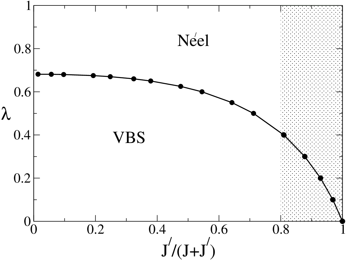
If at $J^{\prime}=0$ we are in the VBS phase (i.e., $n_{c}/N$ is below the critical value (24)), then increasing $\kappa^{(0)}\propto J^{\prime}$ beyond some threshold $\kappa_{c}$ leads to a transition to the Néel phase. On the anisotropic (rectangular) lattice, with the increasing anisotropy (deviation of $\lambda$ from $1$) the transition point $\kappa_{c}$ shifts towards higher values. The resulting phase diagram is shown in Fig. 3. Thus, in two dimensions the $Sp(N)$ perturbation terms in (17) are dangerously irrelevant and can drive the phase transition between the disordered (VBS) and Néel phase.

In one dimension, $y$ always flows to infinity indicating that the system is dimerized in the entire range of $0\leq\kappa<1$, in line with the numerical results. [16] Curiously, in the close vicinity of the uniform $SU(N)$ point $\kappa=1$ ($J^{\prime}\gg J$), the coupling $y$ again exhibits the “U-turn” behavior as described above, and the intermediate scale $l^{*}$ seems to diverge as $J/J^{\prime}\to 0$. This agrees with the fact the uniform $SU(N)$ antiferromagnet $\kappa=1$ is gapless in $d=1$ (it corresponds to the exactly solvable Uimin-Lai-Sutherland (ULS) model[19]).

With the present approach, we are not able to detect any tendency towards a transition to the VBS phase with increasing $J^{\prime}/J$ for the case of isotropic square lattice (line $\lambda=1$). One has to keep in mind that our construction of smooth fields becomes increasingly inadequate as $J\to 0$; however, one can argue that the theory still remains valid at the energy scales of less than order $J$. Several numerical results using exact diagonalization on small 2d clusters, [42] series expansions,[43] and density matrix renormalization group (DMRG) on a ladder [44] suggest that the uniform $SU(4)$ antiferromagnet ($J=0$, $\lambda=1$) is in a VBS phase with the plaquette-type dimerization order. At the same time, theoretical studies advocate different scenarios for the uniform $SU(N)$ antiferromagnetic point: in a recent work based on the Majorana fermion representation of spin-orbital operators,[45] the existence of a $Z_{2}$ spin-orbital liquid state with emergent nodal fermions has been proposed for $N=4$; other studies based on Schwinger-boson representations [46, 47] and exact diagonalization for the $SU(3)$ case[47] suggest that at this point the ground state has the Néel-type $N$-sublattice order, which may be viewed as order at the wavevector $(2\pi/N,2\pi/N)$. The question about the correct ground state around the point $\lambda=1$, $J=0$ is thus still open. Further, our result shown in Fig. 3 indicates that the VBS phase present at small $\lambda$ has the tendency to shrink with increasing $J^{\prime}/J$. This makes plausible to assume that, even if the point $\lambda=1$, $J=0$ is in the VBS state, this phase should be different from the VBS phase at small $\lambda$. Another argument in favor of this scenario is the following: consider the point $J=0$, $\lambda=0$ which describes uncoupled ULS chains. Each chain is gapless, with zero gap at wave vectors $k=2\pi m/N$, $-N/2<m\leq N/2$. Switching on weak interaction $\lambda$ between the chains may be expected to lead to an immediate ordering at those wave vectors, while switching on weak $J$ leads to a VBS state.

Let us now add the quadratic Zeeman field term (19) to the effective model (17) with $N=4$. Now the first and the fourth field components become massive and can be integrated out at once. We decompose the field into the background part $\bm{\varphi}$ and the “fast” massive part $\bm{\chi}$ as follows:

where $\bm{\varphi}^{*}\cdot\bm{\varphi}=1$. One can straightforwardly show that for the two-component unit complex vector field the following identity holds:

Thus, integrating out $\bm{\chi}$, one obtains the familiar $CP^{1}$ model that is equivalent to the $\rm O(3)$ nonlinear sigma model (NLSM) and has been extensively used for a description of Heisenberg spin systems. The topological term (14) is retained. The resulting action takes the form:

The renormalized couplings $g_{1,2}^{*}$ are given by the formulas:

where:

In one and two dimensions one has respectively:

The $CP^{1}$ model with the topological phase angle $\theta=\pi$ has a disordering transition into a gapped dimerized (VBS) phase above a certain critical value $g_{c}$ of the effective coupling $g_{\rm eff}=\sqrt{g_{1}^{*}g_{2}^{*}}$, both in one and two spatial dimensions. For $g_{\rm eff}<g_{c}$, the model is gapless, is long-range ordered in $d=2$ and has quasi-long-range order in $d=1$. Thus, the line of phase transition between the Néel and VBS phases is given by:

Although the exact value of $g_{c}$ is not known, one may expect that Eq. (31) will qualitatively reproduce the transition line.

Fig. 4 shows the result for the case of two dimensions, where we have used $g_{c}=\pi$ (which is just the extrapolation of the large-$N$ result $g_{c}=\frac{2\pi}{N}$ down to the case $N=2$). One can see that the curvature of the phase boundary agrees with the results of the previous section obtained in absence of the field. Again, we cannot see any tendency toward the VBS order at the uniform $SU(N)$ antiferromagnetic point on a square lattice ($J=0$, $\lambda=1$).

In the one-dimensional case, one can do better and extract the value of $g_{c}$ from the comparison with the transition in an antiferromagnetic spin-$\frac{1}{2}$ zigzag chain. Rodriguez et al.[16] have used a direct mapping of the original fermionic model (1) onto an effective spin-$\frac{1}{2}$ chain with nearest- and next-nearest-neighbor exchange couplings $j_{1}$ and $j_{2}$, respectively. The constants $j_{1,2}$ were obtained as series in the perturbation parameter $1/Q$, defined as follows:

Further, by using the value $j_{2}/j_{1}\simeq 0.24$ for the transition point into the dimerized phase, which is known from numerical studies,[48] in Ref. 16 an estimate for the transition line in the $(1-\kappa,Q)$ plane has been obtained that compared very well with the numerical results for the original spin-$\frac{3}{2}$ fermionic model.

In our approach, we can try and fix the value of $g_{c}$ (which is a sole fitting parameter in our theory, for the entire line of transition points in the $(\kappa,q)$ space) by comparing the output of our Eq. (31) to the results of Ref. 16. Fig. 5 shows the transition line obtained from Eq. (31) for $d=1$ with $g_{c}=8.5$ in comparison to the curve obtained in Ref. 16. One can see that the above value of $g_{c}$ yields a good agreement close to the $SU(N)$ antiferromagnetic point $\kappa=0$. So, as a byproduct of our studies of the $Sp(4)$ Heisenberg model, we obtain an independent estimate of the critical coupling value for the 1d $\rm CP^{1}$ model (or, alternatively, the $\rm O(3)$ NLSM) at the topological angle $\theta=\pi$:

In the vicinity of the Sutherland point $J=0$ our description breaks down; this can be seen already from the fact that the transition line goes to a finite value of $q_{0}=2q/J$ at $J\to 0$ (see the inset of Fig. 5), while the main scale in this limit is $J^{\prime}\gg J$, so the critical value of $q_{0}$ should diverge as $(1-\kappa)^{-1}$ in this limit.

We have considered the model (1) describing spin-$\frac{3}{2}$ fermions in a spatially anisotropic optical lattice shown in Fig. 1 at quarter filling in the Mott limit of the on-site repulsion constants $U_{0,2}$ being much larger than the hopping amplitudes $t$. In this limit the charge degrees of freedom have a large gap, and the system can be mapped to the so-called $Sp(4)$ Heisenberg spin model.

We have studied its large-$N$ generalization, the $Sp(N)$ spin model, with the help of the field-theoretical approach constructed in the vicinity of the staggered $SU(N)$ antiferromagnetic point. It is shown that the effective field theory corresponds to the $Sp(N)$ extension of the $CP^{N-1}$ model, with the Lorentz invariance generically broken by the $Sp(N)$ terms that break the $SU(N)$ symmetry. For this effective field theory, we have obtained the renormalization group equations to one-loop order and have shown that although in the vicinity of the staggered $SU(N)$ antiferromagnetic point the $Sp(N)$ terms are seemingly irrelevant, their presence leads to a considerable renormalization of the $SU(N)$ part of the action, thus driving the transition between the phase with a long-range Néel-type order and the magnetically disordered valence bond solid (VBS) phase. We would like to note that solutions of the renormalization group equations in the disordered phase exhibit a characteristic double-scale behavior close to the Néel-VBS transition boundary. Such a behavior is reminiscent to that encountered in other frustrated models,[40, 41] and is also expected[49, 50] in the framework of the deconfined criticality conjecture.[51]

In addition to the $Sp(N)$ perturbation, we have also analyzed the effect of the external magnetic field (quadratic Zeeman effect) and established the qualitative form of the phase diagrams in one and two spatial dimensions. For the physical case $N=4$, at large values of the quadratic Zeeman field the effective theory reduces to $CP^{1}$ model describing an isotropic Heisenberg antiferromagnet with a pseudospin $\frac{1}{2}$. Its ground state in two dimensions is always in the long-range ordered (Néel) phase for the pseudospin-$\frac{1}{2}$, and when the field is decreased, this state either adiabatically evolves into the Néel phase of spin-$\frac{3}{2}$ fermions (with the reduced Néel order[29]) or undergoes a phase transition into the VBS state. In one dimension, there is a phase transition of the Berezinskii-Kosterlitz-Thouless type that corresponds to the spontaneous dimerization transition in a frustrated spin-$\frac{1}{2}$ chain with next-nearest neighbor exchange.[16] As a byproduct, by fitting our results to the available numerical data,[16] we have obtained an estimate for the critical coupling of the $CP^{1}$ model with the $\theta=\pi$ topological term in $(1+1)$ dimensions.

One last word of caution is in order: since our effective theory is constructed around the staggered $SU(N)$ antiferromagnetic point $J^{\prime}=0$, it is not expected to work well close to the other, uniform antiferromagnetic $SU(N)$ point $J=0$. For that reason, we cannot exclude the presence of another phase transition to the VBS phase in some region around the uniform $SU(N)$ point on the isotropic lattice ($J=0$, $\lambda=1$), as suggested in Ref. 17. Constructing an effective field theory describing the vicinity of the uniform antiferromagnetic $SU(N)$ point remains a challenge for the future work.

References

- [1] M. Lewenstein, A. Sanpera, V. Ahufinger, B. Damski, A. Sen(De), and U. Sen, Adv. Phys. 56, 243 (2007).
- [2] I. Bloch, J. Dalibard, and W. Zwerger, Rev. Mod. Phys. 80, 885 (2008).
- [3] T. B. Ottenstein, T. Lompe, M. Kohnen, A. N. Wenz, and S. Jochim, Phys. Rev. Lett. 101, 203202 (2008).
- [4] J. H. Huckans, J. R. Williams, E. L. Hazlett, R. W. Stites, and K. M. O’Hara, Phys. Rev. Lett. 102, 165302 (2009).
- [5] A. N. Wenz, T. Lompe, T. B. Ottenstein, F. Serwane, G. Zürn, and S. Jochim, Phys. Rev. A 80, 040702(R) (2009).
- [6] G. Modugno, F. Ferlaino, R. Heidemann, G. Roati, and M. Inguscio, Phys. Rev. A 68, 011601(R) (2003).
- [7] L.-W. He, C. E. Burkhardt, M. Ciocca, J. J. Leventhal, and S. T. Manson, Phys. Rev. Lett. 67, 2131 (1991).
- [8] T. Fukuhara, Y. Takasu, M. Kumakura, and Y. Takahashi, Phys. Rev. Lett. 98, 030401 (2007).
- [9] J. B. Marston and I. Affleck, Phys. Rev. B 39, 11538.
- [10] A. V. Gorshkov, M. Hermele, V. Gurarie, C. Xu, P. S. Julienne, J. Ye, P. Zoller, E. Demler, M. D. Lukin, and A. M. Rey, Nature Physics 6, 289, (2010).
- [11] M. Hermele, V. Gurarie, and A.M. Rey, Phys. Rev. Lett. 103, 135301 (2009).
- [12] C. Wu, J.-P. Hu, and S.-C. Zhang, Phys. Rev. Lett. 91 186402 (2003).
- [13] P. Lecheminant, E. Boulat, and P. Azaria, Phys. Rev. Lett. 95, 240402 (2005).
- [14] C. Wu, Phys. Rev. Lett. 95, 266404 (2005).
- [15] C. Wu, Mod. Phys. Lett. B 20, 1707 (2006).
- [16] K. Rodriguez, A. Argüelles, M. Colomé-Tatché, T. Vekua, and L. Santos, Phys. Rev. Lett. 105, 050402 (2010).
- [17] Y. Qi and C. Xu, Phys. Rev. B 78, 014410 (2008).
- [18] N. Read and S. Sachdev, Phys. Rev. B 42, 4568 (1990).
- [19] G. V. Uimin, JETP Lett. 12, 225 (1970); C. K. Lai, J. Math. Phys. 15, 1675 (1974); B. Sutherland, Phys. Rev. B 12, 3795 (1975).
- [20] N. Read and S. Sachdev, Phys. Rev. Lett. 66, 1773 (1991).
- [21] F. D. M. Haldane, Phys. Rev. Lett. 61, 1029 (1988).
- [22] N. Read and S. Sachdev, Nucl. Phys. B316, 609 (1989).
- [23] H. Eichenherr, Nucl. Phys. B146, 215 (1978).
- [24] V. L. Golo and A. M. Perelomov, Phys. Lett. B 79, 112 (1978).
- [25] A. D’Adda, M. Lüscher, and P. Di Vecchia, Nucl. Phys. B146, 63 (1978).
- [26] E. Witten, Nucl. Phys. B149, 285 (1979).
- [27] I. Ya. Aref’eva and S. I. Azakov, Nucl. Phys. B162, 298 (1980).
- [28] F. F. Assaad, Phys. Rev. B 71, 075103 (2005).
- [29] N. Kawashima and Y. Tanabe, Phys. Rev. Lett 98, 057202 (2007).
- [30] K. S. D. Beach, F. Alet, M. Mambrini, and S. Capponi Phys. Rev. B 80, 184401 (2009).
- [31] F. D. M. Haldane: Phys. Lett. A 93, 464 (1983); Phys. Rev. Lett. 50, 1153 (1983).
- [32] R. Shankar and N. Read, Nucl. Phys. B336, 457 (1990).
- [33] I. Affleck, Phys. Rev. Lett. 66, 2429 (1991).
- [34] V. Azcoiti, G. Di Carlo, and A. Galante, Phys. Rev. Lett. 98, 257203 (2007).
- [35] D. Schuricht and S. Rachel, Phys. Rev. B 78, 014430 (2008).
- [36] K. Kataoka, S. Hattori, and I. Ichinose, preprint arXiv:1003.5412v1
- [37] C. Xu, Phys. Rev. B 78, 054432 (2008).
- [38] A. M. Polyakov: Phys. Lett. B 59, 87 (1975)
- [39] D. P. Arovas and A. Auerbach, Phys. Rev. B 38, 316 (1988).
- [40] S. Rao and D. Sen, Nucl. Phys. B 424, 547 (1994).
- [41] P. Azaria, P. Lecheminant, and D. Mouhanna, Nucl. Phys. B 455, 648 (1995)
- [42] M. V. D. Bossche, F. C. Zhang, and F. Mila, Eur. Phys. J. B 17, 367 (2000).
- [43] E. Zasinas, O. P. Sushkov, and J. Oitmaa, Phys. Rev. B 64, 184431 (2001).
- [44] S. Chen, C. Wu, S.-C. Zhang, and Y. Wang, Phys. Rev. B 72, 214428 (2005).
- [45] F. Wang and A. Vishwanath, Phys. Rev. B 80, 064413 (2009).
- [46] Shun-Qing Shen, Phys. Rev. B 66, 214516 (2002).
- [47] T. A. Toth, A. M. Läuchli, F. Mila, and K. Penc, arXiv:1009.1398 (unpublished).
- [48] K. Okamoto and K. Nomura, Phys. Lett. A 169, 433 (1992).
- [49] G. Murthy and S. Sachdev, Nucl. Phys. B 344, 557 (1990).
- [50] O. I. Motrunich and A. Vishwanath, Phys. Rev. B 70, 075104 (2004).
- [51] T. Senthil, A. Vishwanath, L. Balents, S. Sachdev, and M. P. A. Fisher, Science 303, 1490 (2004).