On Optimal Deadlock Detection Scheduling

The distributed deadlock problem [8, 20, 16, 26, 11, 14] arises from resource contention introduced by concurrent processes in distributed computational environments. It has received a great deal of attention in different areas such as distributed computing theory [22, 26, 9], distributed database [17, 14, 8, 10, 11], and parallel and distributed simulation [2, 28, 21]. A deadlock is a persistent and circular-wait condition, where each process involved in a deadlock waits indefinitely for resources held by other processes while holding resources needed by others. As a result, none of the processes waiting for needed resources can continue computation any further without obtaining the waited-for resources. A deadlock has an adverse performance effect that offsets the advantages of resource sharing and processing concurrency.

There are three common strategies of dealing with the deadlock problem: deadlock prevention, deadlock avoidance, and deadlock detection and resolution. It is a long-held consensus that both deadlock prevention and deadlock avoidance strategies are conservative and less feasible in handling the deadlock problem in general, whereas the deadlock detection/resolution strategy is widely accepted as an optimistic and feasible solution to the deadlock problem, because of its exclusion of the unrealistic assumption about resource allocation requirements of the processes [10, 16, 26, 7, 27]. The central idea behind the deadlock detection and resolution strategy is that it does not preclude the possibility of deadlock occurring but leaves the burden of minimizing the adverse impact of deadlock to deadlock detection and resolution mechanisms. Under this scheme, the presence of deadlocks is detected by a periodic initiation of a deadlock detection algorithm and then resolved by a deadlock resolution algorithm [31, 27, 7].

Despite significant performance improvement in the past, deadlock detection remains a costly operation [26, 11, 19]. It requires dynamical maintenance of wait-for-graph (WFG) that reflects the runtime wait-for dependency among distributed processes, and performs a graph analysis to detect the presence of deadlocks. There is a substantial tradeoff between the cost of deadlock detection and that of deadlock resolution [26, 16, 23]. An initiation of deadlock detection consumes runtime system and network resources which are basically pure overheads when no deadlock is present [26, 19]. Excessive initiation of deadlock detection would reduce the deadlock resolution cost but result in system performance degradation in the absence of deadlock, while infrequent deadlock detection would be accompanied by the increased deadlock size, resulting in an increased deadlock resolution cost in the presence of deadlocks [23, 16, 15, 1]. It is evident that deadlock detection scheduling is one of key factors affecting the overall system performance of deadlock handling. Nevertheless, to the best of our knowledge, this subject is generally missing in the literature.

This paper investigates the optimal deadlock detection scheduling. We study how to best schedule deadlock detections so as to minimize the long-run mean average cost of deadlock handling. We formulate this problem by introducing a generic cost model (utility metric) and use this cost model to establish a connection between deadlock detection and deadlock resolution costs, in relation to the rate of deadlock formation. We show that there exists a unique optimal deadlock detection frequency that yields the minimum long-run mean average cost. Moreover, our result indicates that the asymptotically optimal frequency of deadlock detection that minimizes the message overhead is ${\cal O}((\lambda n)^{1/3})$, when the number $n$ of processes in the system is sufficiently large. In addition, we prove that a fully distributed (uncoordinated) detection scheduling can not be performed as efficiently as its centralized counterpart (coordinate scheduling).

The rest of this paper is organized as follows. Section 2 contains a brief summary of the distributed deadlock detection and resolution algorithms. Section 3 gives the notions and definitions. Section 4 provides the detailed mathematical analysis and proves the existence and uniqueness of an optimal detection frequency. The determination of the optimal deadlock detection frequency, its asymptotic relation with the number of processes in a distributed system, and the impact of random detection scheduling upon the long-run mean average cost of deadlock handling, are presented. In Section 5, the main contribution of this paper is highlighted and the possible future work is discussed.

In this section we provide a brief summary of worst-case analysis of existing distributed detection algorithms of generalized deadlocks and deadlock resolution algorithms since some results will be used later on. We also touch on Gray’s simulation model [8] as well as Massey’s formulation [20].

We restrict our discussion to distributed detection and resolution algorithms. The references [10, 12, 13, 11, 14, 16] provide excellent gateways to the state of the art in this area for the generalized resource request model. In the following, we give a brief summary of the worst-case performance of the existing distributed detection algorithms.

Table 1 summarizes the worst-case complexities of distributed deadlock detection algorithms [3, 30, 12, 14], where $n$ is the total number of processes, $e$ the number of edges, $d$ the diameter, and $l$ the number of sink nodes of the WFG. The distributed detection algorithm for generalized deadlocks by Kshemkalyni and Singhal [14] is the clear winner among the algorithms listed in Table 1. Their algorithm has achieved a message complexity of $2e$ and a time complexity of $2d$, which are believed to be optimal. Since $e=n(n-1)$ and $d=n$ in the worst-case analysis, the worst-case message complexity and time complexity thus can be written as $2n^{2}$ and $2n$, respectively.

Although deadlock detection and deadlock resolution are often discussed separately, the latter is as important as the former [10, 26, 12, 7, 27, 32, 16]. The primary issue of deadlock resolution [15, 16, 17] is to selectively abort a subset of processes involved in the deadlock so as to minimize the overall abortion cost [19, 26, 27, 7]. This is often referred to as the minimum abort set problem. These victim (aborted) processes must cancel all pending requests and release all the acquired resources in order to avoid false deadlock detection and resolution [26, 12, 7]. The abortion cost thus includes (1) the sending of cancel messages to those resources, and (2) the sending of reply messages to all the waiting processes that are currently being blocked for the resources held by the aborted processes. One noteworthy point is that these waiting processes could be either transitively blocked or deadlocked processes. To further reduce the abortion cost, checkpointing is sometimes introduced to prevent the victim processes from being rolled back from scratch [18].

By transforming the problem of deadlock resolution into a minimum vertex cut problem, Lin & Chen’s algorithm [5] can identify an optimal set of victim processes to be aborted, with the properly selected abortion cost to avoid the starvation and livelock problems. The main feature of Terekhov & Camp’s algorithm is to take the number of resources into account. The deadlock resolution algorithm proposed by Mendivil et al. [7] uses a probe-based approach, with a focus on the safety aspect of deadlock resolution. The novelty of this algorithm is to use an additional round of message exchanges to gather the information needed for efficient resolution after deadlocks are detected. The algorithm uses special message known as probes to travel in the opposite direction of the edges in AWFG (asynchronous wait-for graph), and then chooses the lowest priority process of each detected cycle as a victim process to be aborted, hence avoiding the livelock and starvation problems. This deadlock resolution algorithm [7] excels in the use of formal methods to prove the correctness and in its fine-granular analysis of the algorithm complexities. In particular, its message complexity is of ${\cal O}(mn^{2}_{D})$. The worst-case message complexity can also be written as ${\cal O}(n^{3})$ because the eventual deadlock size, $n_{D}$, is bounded by the total number of processes in the distributed system, that is, $m={\cal O}(n)$ and $n_{D}={\cal O}(n)$.

The past research has been primarily aimed at minimizing the complexities (costs) of the deadlock detection and resolution algorithms. Although deadlock detection scheduling (particularly how frequently deadlock detection should be performed) has significant impact on the overall performance of deadlock handling in practice, it is not explicitly studied but rather implicitly reflected in the description of deadlock detection algorithms, without a clear guideline. For instance, in [10, 26, 14, 16, 19, 4, 10, 5], the authors stated that a deadlock detection is initiated when a deadlock is suspected. Other works [23, 11] suggested that it would be highly inefficient if deadlock detection is performed whenever a process/transaction becomes blocked.

The performance of deadlock handling not only depends on the per-detection cost of the deadlock detection algorithm, but also on how frequently the deadlock detection algorithm is executed [11, 23, 19]. The choice of deadlock detection frequency presents a tradeoff between deadlock detection cost and deadlock resolution cost [10, 26, 23, 16, 11]. Park et al. [23] pointed out that the reduction of deadlock resolution cost can be achieved at the expense of deadlock detection cost. Krivokapie et al. [11] showed in their simulation study that the path-pushing algorithm (one type of deadlock detection algorithm) is highly sensitive to the frequency of deadlock detection. Gray et al. [8] showed that the probability of a transaction waiting for a lock request is rare. They used a “straw-man analysis” in their simulation model that agreed well with the observation on several data management systems. Massey [20] formulated a probabilistic model that gave an analytic justification for the simulation results reported in [8], showing that the probability of deadlock grows linearly with respect to the number of transactions and grows in the fourth power of the average number of resources required by transactions.

To our best knowledge, only a few papers [8, 16, 27, 5, 26, 19, 6] mentioned about deadlock detection scheduling but under a different context from this paper. The idea of relating deadlock recovery cost to deadlock persistence time, and identifying an optimal deadlock detection frequency that minimizes the long-run mean average cost from the perspective of deadlock handling, has not been considered before.

In this section, we first give the following definitions in order to simplify problem formulation.

The independence of deadlock occurrence can be justified by the wide acceptance of large-scale distributed systems and adoption of fine-granularity locking mechanism such as semantic locking [24, 11] and record-granularity locking [24]. After decades of research and development, large-scale distributed systems allow resource sharing among hundreds or even thousands of sites across a network [24, 11]. The fine-granular locking mechanisms enable a higher degree of parallelism. Large-scale resource distribution and fine-granularity of locking make deadlocks likely to form independently.

The function $t_{p}(t,S_{i})$ represents the time interval between the present time and the time at which the deadlock is initially formed. It grows linearly until the deadlock is resolved. The notion of deadlock persistence time in spirit is similar to that of deadlock latency or deadlock duration in [16, 15].

Once a deadlock is formed, other processes requesting resources currently held by the blocked processes in the deadlock (including deadlocked and transitively blocked processes) will be blocked forever unless the deadlock is resolved. As a result, each deadlock acts as an attractor to trap more processes into it. As the deadlock persistence time increases, the size of the deadlock (the total number of processes involved in the deadlock) keeps growing [26, 9, 16, 15], which in turn increases the deadlock resolution cost.

Throughout this paper, we use $n$ to denote the total number of processes in a distributed system and $n_{D}(.)$ to denote the size of a deadlock. Consider an arbitrary deadlock. Its size is a function of deadlock persistence time $t_{p}$, denoted as $n_{D}(t_{p})$. The deadlock size $n_{D}(t_{p})$ by nature is a discrete staircase function that jumps by one whenever a new process becomes transitively blocked by the deadlocked processes. To facilitate our mathematical analysis, we will treat $n_{D}(t_{p})$ instead as a continuous, increasing function, which is an approximation of the staircase one.

The deadlock size function $n_{D}(t_{p})$ has the following mathematical properties. (1) $n_{D}(0)=0$, (2) monotonicity: $n_{D}^{\prime}(t_{p})>0,\ t_{p}\geq 0$, and (3) bounded: $n_{D}(\infty)\leq n$, where $n^{\prime}_{D}(t_{p})$ is the derivative of $n_{D}(t_{p})$. The first property refers to the initial deadlock size at $t_{p}=0$ is zero. The second property reflects the fact that the number of blocked processes in the deadlock increases monotonically with deadlock persistence time $t_{p}$, and the third property indicates that the eventual deadlock size is bounded by the total number of distributed processes. For the sake of easy presentation, we drop the subscript $p$ hereafter.

Now let’s revisit the message complexity achieved by the deadlock resolution algorithm proposed by Mendivil et al. [7], which is ${\cal O}(mn_{D}^{2})={\cal O}(nn_{D}^{2})$, where $m$ is the number of deadlocked processes having priority values greater than those of the deadlocked processes. Notice that the deadlock size, $n_{D}$, is a function of deadlock persistence time. To make this dependency concrete, the message overhead can be written as $cnn^{2}_{D}(t)$ for some constant $c$. This result will be used later to derive the optimal frequency of deadlock detection scheduling.

In this section, we begin with a generic cost model that accounts for both deadlock detection and deadlock resolution, which is independent of deadlock detection/resolution algorithms being used. We then prove the existence and the uniqueness of an optimal deadlock detection frequency that minimizes the long-run mean average cost in terms of the message complexities of the best known deadlock detection/resolution algorithms.

In this paper we choose the message complexity as the performance metric for measuring the detection/resolution cost. The reason for choosing message complexity is that communication overhead is generally a dominant factor that affects the overall system performance in a distributed system [26, 10, 13, 14], as compared with processing speed and storage space. Note that the worst-case message complexity can normally be expressed as a polynomial of $n$. Per deadlock detection cost is denoted as $C_{D}$. The resolution cost for a deadlock is denoted as $C_{R}(t)$, which is a function of the deadlock persistence time $t$. In general, the resolution cost is a polynomial of $n_{D}(t)$. For example, the deadlock resolution cost for Mendivil’s algorithm [7] is $cnn^{2}_{D}(t)$. Because $n_{D}(t)$ is a monotonically increasing function of deadlock persistence time. $C_{R}(t)$ is also monotonically increasing with deadlock persistence time. We assume that deadlock formation follows a Poisson process for two reasons: First, the Poisson process is widely used to approximate a sequence of events that occur randomly and independently. Second, it is due to mathematical tractability of the Poisson process, which allows us to characterize the essential aspects of complicated processes while making the problem analytically tractable.

The following theorem presents the long-run mean average cost of deadlock handling in connection with the rate of deadlock formation and the frequency of deadlock detection.

Let $N(t)=\sup\{n:~S_{n}\leq t\}$ represent the number of deadlock occurrences within the time interval $(0,t]$. The long-run mean average cost is

$$\lim\limits_{t\to\infty}\frac{E(\hbox{random~cost~in~}(0,t])}{t},$$

(2)

where $E$ is the expectation function. In order to associate this cost with the deadlock detection frequency ($1/T$), we partition the time interval $(0,t]$ into non-overlapping subintervals of length $T$. Let $\xi_{k}(T)$ be the cost of deadlock handling on the subinterval $((k-1)T,kT],\ k>0$. $\xi_{k}(T)$ is a random variable. According to the stationary and independent increments of Poisson process [25], $E(\xi_{i}(T))=E(\xi_{j}(T)),\ i\neq j$. The long-run mean average cost becomes

	$\displaystyle C(T)$	$\displaystyle=\lim\limits_{t\to\infty}\frac{E(\hbox{random~cost~in~}(0,t])}{t}=\lim\limits_{t\to\infty}\frac{E(\sum\limits_{k=0}^{\lfloor\frac{t}{T}\rfloor}\xi_{k}(T))}{t}$
		$\displaystyle=\lim\limits_{t\to\infty}\frac{E(\lfloor\frac{t}{T}\rfloor\xi_{1}(T))}{t}=\frac{E(\xi_{1}(T))}{T},$		(3)

where $\lfloor x\rfloor$ is the floor function in $x$.

The cost $\xi(T)$ on interval $(0,T]$ is the sum of a deadlock detection cost $C_{D}$ and a deadlock resolution cost for those deadlocks independently formed within the interval $(0,T]$. For the ith deadlock formed at time $S_{i}\leq T$, the resolution cost $C_{R}(T-S_{i})$ is a function of the deadlock persistence time $T-S_{i}$. Hence, the accrued total cost over $(0,T]$ is

$\displaystyle\xi(T)=C_{D}+\sum\limits^{N(T)}_{i=1}C_{R}(T-S_{i})I_{\{N(T)>0\}},$

(4)

where $I_{\theta}$ is the indicator function whose value is 1 (or 0) if predicate $\theta$ is true (or false). Among that, the deadlock resolution cost on interval $(0,T]$ is

$\displaystyle\sum\limits^{N(T)}_{i=1}C_{R}(T-S_{i})I_{\{N(T)>0\}}=\sum\limits^{\infty}_{i=1}C_{R}(T-S_{i})I_{\{S_{i}\leq T\}}$

(5)

$\displaystyle E\left(C_{R}(T-S_{i})I_{\{S_{i}\leq T\}}\right)=\int\limits^{T}_{0}C_{R}(T-t)f_{i}(t)dt$

(6)

where $f_{i}(t)$ is the probability density function of $S_{i}$ which follows the gamma distribution given below:

$$f_{i}(t)=\frac{\lambda^{i}}{(i-1)!}t^{i-1}e^{-\lambda t},~t>0.$$

(7)

Substituting Eq(7) into Eq(6) gives rise to

$\displaystyle E\left(C_{R}(T-S_{i})I_{\{S_{i}\leq T\}}\right)=\int^{T}_{0}C_{R}(T-t)\frac{\lambda^{i}}{(i-1)!}t^{i-1}e^{-\lambda t}dt.$

(8)

The expected total resolution cost over the time interval $(0,T]$ is

		$\displaystyle E(\sum\limits^{N(T)}_{i=1}C_{R}(T-S_{i})I_{\{N(T)>0\}})=\sum\limits^{\infty}_{i=1}\int^{T}_{0}C_{R}(T-t)\frac{\lambda^{i}t^{i-1}}{(i-1)!}e^{-\lambda t}dt$
		$\displaystyle=\int^{T}_{0}C_{R}(T-t)\lambda e^{-\lambda t}\left(\sum\limits^{\infty}_{i=1}\frac{(\lambda t)^{i-1}}{(i-1)!}\right)dt=\lambda\int^{T}_{0}C_{R}(T-t)dt=\lambda\int^{T}_{0}C_{R}(t)dt.$		(9)

Combining Eqs(3), (4), and (9) yields

$\displaystyle C(T)=\frac{E(\xi_{1}(T))}{T}=\frac{C_{D}}{T}+\frac{\lambda\int^{T}_{0}C_{R}(T-t)dt}{T}=\frac{C_{D}}{T}+\frac{\lambda\int^{T}_{0}C_{R}(t)dt}{T}.$

(10)

Theorem 1 is thus established. $\blacksquare$

Theorem 1 is mainly concerned with the impact of deadlock detection frequency and deadlock formation rate on the long-run mean average cost of overall deadlock handling. It is independent of the choice of deadlock detection/resolution algorithms. The following corollary is an immediate consequence of Theorem 1.

Proof: the proof is straightforward and thus omitted. $\blacksquare$

Theorem 1 and Corollary 1 state that the overall cost of deadlock handling is closely associated not only with per-deadlock detection cost, and aggregated resolution cost, but also with the rate of deadlock formation, $\lambda$. In the following lemma, we will show the existence and uniqueness of asymptotic optimal frequency of deadlock detection when deadlock resolution is more expensive than a deadlock detection in terms of message complexity.

Proof: Differentiating Eq(1) yields

$$C^{\prime}(T)=-\frac{C_{D}}{T^{2}}+\frac{\lambda C_{R}(T)}{T}-\frac{\lambda\int^{T}_{0}C_{R}(t)dt}{T^{2}}.$$

(11)

Define a function $\varphi(T)$ as follows

$\displaystyle\varphi(T)\equiv T^{2}C^{\prime}(T)=-C_{D}+\lambda TC_{R}(T)-\lambda\int^{T}_{0}C_{R}(t)dt.$

(12)

Notice that $C^{\prime}(T)$ and $\varphi(T)$ share the same sign. Differentiating $\varphi(T)$, we have

$\displaystyle\varphi^{\prime}(T)=\lambda TC_{R}^{\prime}(T)$

(13)

To make the idea behind this derivation concrete, we apply the up-to-date results of deadlock detection/resolution algorithms. As discussed before, the best-known message complexity of a distributed deadlock detection algorithm is $2n^{2}$ [14] when it is written as a polynomial of $n$. The best-known message complexity of a deadlock resolution algorithm is ${\cal O}(nn_{D}^{2})$ [7]. Therefore, $C_{D}=n^{2}$, and $C_{R}(t)=cnn^{2}_{D}(t)$, where $c$ is a positive constant. Because the deadlock size $n_{D}(t)$ is always bounded by $n$, from (15) we have

$\displaystyle\varphi(\infty)=\lim\limits_{T\to\infty}\varphi(T)>-C_{D}+\lambda\xi(C_{R}(\infty)-C_{R}(\xi))\approx-2n^{2}+\lambda c\xi n^{3}.$

(18)

Note that $\xi$ is a fixed value that can be arbitrarily chosen. For a sufficiently large $n$, Eq(18) becomes

$\displaystyle\varphi(\infty)\approx\lambda c\xi n^{3}>0$

(19)

$\varphi(0)=-C_{D}=-2n^{2}$. Because $\varphi(T)$ is monotonically increasing, there exists an optimal deadlock detection frequency $1/T^{*}$ such that $\varphi(T^{*})$ and thus $C^{\prime}(T^{*})$ are zero, which minimizes the long-run mean average cost $C(T)$ for deadlock handling.

The motivation behind the proof is that the cost per deadlock detection is fixed when the total number of processes in the distributed system is given, while the cost of deadlock resolution monotonically increases with deadlock persistence time. The resolution cost will eventually outgrow the detection cost if deadlocks persist. As we set the time interval $T$ between any two consecutive detections longer, the detection cost becomes smaller due to less frequent executions of the detection algorithm, but the resolution cost becomes larger due to the growth in deadlock size. This implies that there exists a unique deadlock detection frequency $1/T^{*}$ that balances the two costs such that their sum is minimized. The condition that the asymptotic deadlock resolution cost, $C_{R}(\infty)$, is greater than the cost of deadlock detection, $C_{D}$, constitutes the natural mathematical basis to justify distributed deadlock detection algorithms.

We are now ready to state the asymptotically optimal frequency for deadlock detection based on the up-to-date results of distributed deadlock detection and resolution algorithms. Recall that the best-known message complexity for distributed deadlock detection algorithms is $2n^{2}$ [14] and that for deadlock resolution algorithms of ${\cal O}(nn_{D}^{2})$ [7].

By the properties of the deadlock size function $n_{D}(t)$, we have $n_{D}(0)=0$ and $n^{\prime}_{D}(0)>0$. It can be easily verified that $c_{0}=0$ and $c_{1}=n^{\prime}_{D}(0)>0$. The resolution cost $C_{R}(t)$ can be written as $cnn^{2}_{D}(t)$ for some constant $c$. By Theorem 1, the long-run mean average cost becomes

$$C(T)=\frac{2n^{2}}{T}+\lambda cn\frac{\int_{0}^{T}n^{2}_{D}(t)dt}{T}.$$

(21)

Inserting Eq(20) into Eq(21), we have

$\displaystyle C(T)=$

$\displaystyle\frac{2n^{2}}{T}+\lambda cn^{3}T^{-1}\int_{0}^{T}(\sum_{i=1}^{\infty}c_{i}t^{i})^{2}dt=\frac{2n^{2}}{T}+\frac{\lambda cn^{3}\int_{0}^{T}(c_{1}t+\sum_{i=2}^{\infty}c_{i}t^{i})^{2}dt}{T}.$

(22)

Through a lengthy calculation, Eq(22) can be simplified as

$\displaystyle C(T)$

$\displaystyle=\frac{2n^{2}}{T}+c\lambda n^{3}(\frac{c_{1}^{2}T^{2}}{3}+\frac{2c_{1}c_{2}T^{3}}{4})+c\lambda n^{3}(\sum_{i=2}^{\infty}\sum_{j=2}^{\infty}\frac{c_{i}c_{j}T^{i+j}}{i+j+1}).$

(23)

Taking derivative of Eq(23) with respect to $T$, we have

$\displaystyle C^{\prime}(T)$

$\displaystyle=-\frac{2n^{2}}{T^{2}}+c\lambda n^{3}(c^{2}_{1}\frac{2T}{3}+\frac{3c_{1}c_{2}T^{2}}{2})+c\lambda n^{3}(\sum_{i=2}^{\infty}\sum_{j=2}^{\infty}\frac{c_{i}c_{j}(i+j)T^{i+j-1}}{i+j+1}).$

(24)

By lemma 1, there exists a unique optimal detection frequency $1/T^{*}$ when $n$ is sufficiently large, such that $C(T^{*})\leq C(T),\ \ T\in(0,\infty)$. We know that $C^{\prime}(T^{*})=0$. Based on (24), we transform $C^{\prime}(T^{*})=0$ to the following equation.

$\displaystyle\frac{1}{n}=\frac{c\lambda}{2}(\frac{2c^{2}_{1}(T^{*})^{3}}{3}+\frac{3c_{1}c_{2}(T^{*})^{4}}{2}+\sum_{i=2}^{\infty}\sum_{j=2}^{\infty}\frac{c_{i}c_{j}(i+j)(T^{*})^{i+j+1}}{i+j+1}).$

(25)

Only $n$, $T^{*}$, and $\lambda$ are free variables and the rest are constants. By performing the Big-O reduction we obtain

$\displaystyle\frac{1}{n}$

$\displaystyle=\Theta(\lambda((T^{*})^{3}+(T^{*})^{4}+(T^{*})^{5}+...))$

(26)

When $n$ is sufficiently large and $T^{*}$ is sufficiently small, we have

		$\displaystyle\frac{1}{n}=\Theta(\lambda\frac{(T^{*})^{3}}{1-T^{*}})={\cal O}(\lambda(T^{*})^{3})$
		$\displaystyle T^{*}=\Omega(\frac{1}{(\lambda n)^{1/3}})$		(27)

Therefore, the asymptotic optimal deadlock detection frequency $1/T^{*}$ is ${\cal O}((\lambda n)^{1/3})$. $\blacksquare$

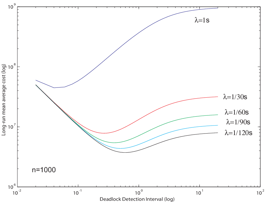
As an illustration, we consider an example as follows. Let $C_{R}(t)=n^{3}(1-\exp(-t))$, $C_{D}=n^{2}$. In accordance with Theorem 1, the long-run mean average cost of deadlock handling thus is written as

$\displaystyle C(T)=\frac{n^{2}+\lambda n^{3}(T+\exp(-T)-1)}{T}.$

(28)

$\#$ of Processes	Optimal Detection Interval ($\lambda=1$)
$50$	$0.214699$(s)
$100$	$0.148555$(s)
$200$	$0.103495$(s)
$500$	$0.064189$(s)
$1000$	$0.045402$(s)
$\#$ of Processes	Optimal Detection Interval ($\lambda=1/30$)
$50$	$2.0223$(s)
$100$	$1.0973$(s)
$200$	$0.6832$(s)
$500$	$0.3942$(s)
$1000$	$0.2675$(s)
Table 1: Optimal Detection Interval vs. $\#$ of Processes

A detailed calculation given in Table 1 shows that as the number of processes in a distributed system increases, the optimal detection interval decreases, which is clearly in line with our theoretical analysis. In the sequel, we study the impact of coordinated vs. random deadlock detection scheduling on the performance of deadlock handling. We consider two strategies of deadlock detection scheduling: (1) centralized, coordinated deadlock detection scheduling, and (2) fully distributed, uncoordinated deadlock detection scheduling.

The centralized scheduling excels in its simplicity in implementation and system maintenance, but undermines the reliability and resilience against failures because one and only one process is elected as the initiator of deadlock detections in a distributed system. In contrast, the fully distributed scheduling excels in the reliability and resilience against failures because every process in the distributed system can independently initiate detections [15], without a single point of failure. However, due to the lack of coordination in deadlock detection initiation among processes, it presents a different mathematical problem from the centralized deadlock detection scheduling.

In the previous discussions we have focused on the derivation of optimal frequency of deadlock detection in connection with the rate of deadlock formation and the message complexities of deadlock detection and resolution algorithms, assuming deadlock detections are centrally scheduled at a fixed rate of $1/T$. To capture the lack of coordination in fully distributed scheduling, we will study the case where processes randomly, independently initiate the detection of deadlocks.

Let $n$ be the number of processes in a distributed system and $T$ be the optimal time interval between any two consecutive deadlock detections in the centralized scheduling. Consider a fully distributed deadlock detection scheduling, where each process initiates deadlock detection at a rate of $1/(nT)$ independently. Although the average interval between deadlock detections in the fully distributed scheduling remains $T$ (the same as its centralized counterpart), the actual occurring times of those detections are likely to be non-uniformly spaced because the initiation of deadlock detection is performed by the processes in a completely uncoordinated fashion.

In the following we will study the fully distributed (random) scheduling and compare it with the centralized scheduling. Consider a sequence of independently and identically distributed iid random variables $\{Y_{i},i\geq 1\}$ defined on $(0,\infty)$ following certain distribution $H$. The sequence $\{Y_{i},i\geq 1\}$ represents the inter-arrival times of deadlock detections initiated by the fully distributed scheduling, and it is assumed to be independent of the arrival of deadlock formations. It is obvious that the centralized scheduling is a special case of the fully distributed scheduling.

Let ${\cal H}$ be the family of all distribution functions on $(0,\infty)$ with finite first moment. Namely,

		$\displaystyle{\cal H}=\left\{H\colon H\hbox{~is~a~CDF~on~$(0,\infty)$,}\int^{\infty}_{0}\bar{H}(t)dt<\infty\right\}$		(29)
		$\displaystyle\hbox{where $\bar{H}(t)\equiv 1-H(t),~\forall t\geq 0$}.$

The following theorem states that the lack of coordination in deadlock detection initiation by fully distributed scheduling will introduce additional overhead in deadlock handling. Therefore the fully distributed scheduling in general cannot perform as efficiently as its centralized counterpart.

Deadlock detection scheduling is an important, yet often overlooked aspect of distributed deadlock detection and resolution. The performance of deadlock handling not only depends upon per-execution complexity of deadlock detection/resolution algorithms, but also depends fundamentally upon deadlock detection scheduling and the rate of deadlock formation. Excessive initiation of deadlock detection results in an increased number of message exchange in the absence of deadlocks, while insufficient initiation of deadlock detection incurs an increased cost of deadlock resolution in the presence of deadlocks. As a result, reducing the per-execution cost of distributed deadlock detection/resolution algorithms alone does not warrant the overall performance improvement on deadlock handling.

The main thrust of this paper is to bring an awareness to the problem of deadlock detection scheduling and its impact on the overall performance of deadlock handling. The key element in our approach is to develop a time-dependent model that associates the deadlock resolution cost with the deadlock persistence time. It assists the study of time-dependent deadlock resolution cost in connection with the rate of deadlock formation and the frequency of deadlock detection initiation, differing significantly from the past research that focuses on minimizing per-detection and per-resolution costs.

Our stochastic analysis, which solidifies the ideas presented in [10, 26, 23, 11], shows that there exists a unique deadlock detection frequency that guarantees a minimum long-run mean average cost for deadlock handling when the total number of processes in a distributed system is sufficiently large, and that the cost of overall deadlock handling grows linearly with the rate of deadlock formation.

In addition, we study the fully distributed (random) deadlock detection scheduling and its impact on the performance of deadlock handling. We prove that in general the lack of coordination in deadlock detection initiation among processes will increase the overall cost of deadlock handling.

Theoretical results obtained in this paper could help system designers/practitioners to better understand the fundamental performance tradeoff between deadlock detection and deadlock resolution costs, as well as the innate dependency of optimal detection frequency upon deadlock formation rate. However, there are still a lot of questions regarding how to use theoretical results to fine-tune the performance of a distributed system. Determination of the actual rate of deadlock formation and verification of the Poisson process are problems of great complexity that can be influenced by many known/unknown factors such as the granularity of locking, actual distribution of resource, process mix, and resource request and release patterns [26]. Tapping into system logging files and inferring the actual deadlock formation rate via data mining could provide an effective and feasible way to translate theoretical insights into actual system performance gain.

We would like to thank Drs. Marek Rusinkiewicz, Wai Chen and Ritu Chadh at Applied Research, Telcordia Technologies for their constructive comments. We are grateful to the anonymous reviewers for critically reviewing the manuscript and for their truly helpful comments. Yibei Ling would like to especially thank Dr. Shu-Chan Hsu in Department of Cell Biology and Neuroscience at Rutgers University for her encouragement and support.

References

- [1] Roberto Baldoni and Silvio Salz. Deadlock Detection in Multidatabase Systems: a Performance Analysis. DIstributed Systems Engineering, 4:244–252, December 1997.
- [2] Azzedine Boukerche and Carl Tropper. A Distributed Graph Algorithm for the Detection of Local Cycles and Knots. IEEE Transactions on Parallel and Distributed Systems, 9(8):748–757, August 1998.
- [3] G. Bracha and S. Toueg. Distributed Deadlock Detection. Distributed Computing, 2:127–138, 1987.
- [4] K.M. Chandy, J. Misra, and L. Hass. Distributed Deadlock. ACM Transaction on Computer Systems, 1(2):144–156, May 1983.
- [5] Shigang Chen, Yi Deng, and Wei Sun. Optimal Dealock Detection in Distributed Systems Based on Locally Constructed Wait-for Graph. In Proceedings of the 16th International Conference on Distributed Computing Systems, pages 613–619, 1996.
- [6] Shigang Chen and Yibei Ling. Stochastic Analysis of Distributed Deadlock Scheduling. In Proceedings of the 24th ACM Symposium on Principles of Distributed Computing, pages 265–273, July 17-20 2005.
- [7] Jose Ramon Gonzales de Mendivil, Jose Ramon Garitagoitia, Carlos F. Alastruey, and J.M. Bernabeu-Auban. A Distributed Deadlock Resolution Algorithm for the AND Model. IEEE Transactions on Parallel and Distributed Systems, 10(5):433–447, May 1999.
- [8] Jim Gray, P. Homan, Ron Obermarck, and Henry Korth. A Straw-man Analysis of the Probability of Waiting and Deadlock in a Database System. IBM Research, RJ3066, February 1981.
- [9] Young M. Kim, Tan H. Lai, and Neelam Soundarajan. Efficient Distributed Deadlock Detection and Resolution Using Probes, Tokens, and Barriers. In Proceedings of the International Conference on Parallel and Distributed Systems, pages 584–591, 1997.
- [10] Edgar Knapp. Deadlock Detection in Distributed Databases. ACM Computing Surveys, 19(4):303–328, 1987.
- [11] Natalija Krivokapic, Alfons Kemper, and Ehud Gudes. Deadlock Detection in Distributed Database Systems: A New Algorithm and a Comparative Performance Analysis. VLDB Journal: Very Large Data Bases, 8(2):79–100, 1999.
- [12] Ajay D. Kshemkalyani and Mukesh Singhal. Efficient Detection and Resolution of Generalized Distributed Deadlocks. IEEE Transactions on Software Engineering, 20(1):43–54, January 1994.
- [13] Ajay D. Kshemkalyani and Mukesh Singhal. Distributed Detection of Generalized Deadlocks. In Proceedings of the 1997 International Conference on Distributed Computing Systems, pages 553–560, 1997.
- [14] Ajay D. Kshemkalyani and Mukesh Singhal. A One-Phase Algorithm to Detect Distributed Deadlocks in Replicated Databases. IEEE Transactions on Knowledge and Data Engineering, 11(6):880–895, 1999.
- [15] Soojung Lee. Fast, Centralized Detection and Resolution of Distributed Deadlocks in the Generalized model. IEEE Transactions on Software Engineering, 30(8):561–573, September 2004.
- [16] Soojung Lee and Junguk L. Kim. Performance Analysis of Distributed Deadlock Dectection Algorithms. IEEE Transactions on Knowledge and Data Engineering, 13(3):623–636, 2001.
- [17] Xuemin Lin and Jian Chen. An Optimal Deadlock Resolution Algorithm in Multidatabase Systems. In Proceedings of the 1996 International Conference on Parallel and Distributed Systems, pages 516–521, 1996.
- [18] Yibei Ling, Jie Mi, and Xiaola Lin. A Variational Calculus Approach to Optimal Checkpoint Placement. IEEE Transactions on Computers, 50(7):699–708, July 2001.
- [19] Philip P. Macri. Deadlock Detection and Resolution in a CODASYL based Data Management System. In Proceedings of the 1976 ACM SIGMOD International Conference on Management of Data, pages 45–49, 1976.
- [20] William A. Massey. A Probabilistic Analysis of a Database System. ACM SIGMETRICS Performance Evaluation Review, 14(1):141–146, 1986.
- [21] Jayadev Misra. Distributed Discrete-Event Simulation. ACM Computing Surveys, 18(1):39–65, March 1986.
- [22] Ron Obermarck. Distributed Deadlock Detection Algorithm. ACM Transactions on Database Systems, 7(2):187–208, June 1982.
- [23] Young Chul Park, Peter Scheuermann, and Snag Ho Lee. A Periodic Deadlock Detection and Resolution Algorithm with a New Graph Model for Sequential Transaction Processing. In Proceedings of the Eighth International Conference of Data Engineering, pages 202–209, February 1992.
- [24] M. Roesler and W. A. Burkhard. Semantic Lock Models in Object-oriented Distributed Systems and Deadlock Resolution. In Proceedings of the 1988 ACM SIGMOD International Conference on Management of Data, pages 361–370, 1988.
- [25] Sheldon M. Ross. Stochastic Processes. John Wiley & Sons, Inc., New York, 1996.
- [26] Mukesh Singhal. Deadlock detection in distributed systems. IEEE Computer Magazine, 40(8):37–48, November 1989.
- [27] Igor Terekhov and Tracy Camp. Time Efficient Deadlock Resolution Algorithms. Information Processing Letters, 69:149–154, 1999.
- [28] Carl Tropper and Azzedine Boukerche. Parallel simulations of communicating finite state machines. In Proceedings of the SCS Multiconf on Parallel and Distributed Simulation, pages 143–150, May 1993.
- [29] Jesus Villadangos, Federico Farina, Jose Ramon Gonzales de Mendivil, Jose Ramon Garitagoitia, and Alberto Cordoba. A Safe Algorithm for Resolving OR Deadlocks. IEEE Transactions on Software Engineering, 29(7):608–622, July 2003.
- [30] J.W. Wang, Shing-Tsaan Huang, and Nian-Shing Chen. A Distributed Algorithm for Detecting Generalized Deadlocks. Technical Report (SF-C-010-1), Computer Science, National Tsing-Hua University, 1990.
- [31] Yi-Min Wang, Michael Merritt, and Alexander B. Romanovsky. Guaranteed Deadlock Recovery: Deadlock Resolution with Rollback Propagation. In Technical Report Number 648, 1998.
- [32] Sugath Warnakulasuriya and Timothy Mark Pinkston. A Formal Model of Message Blocking and Deadlock Resolution in Interconnection Networks. IEEE Transactions on Parallel and Distributed Systems, 11(3):212–229, March 2000.