Modeling Network Coded TCP Throughput:
A Simple Model and its Validation
Abstract
We analyze the performance of TCP and TCP with network coding (TCP/NC) in lossy wireless networks. We build upon the simple framework introduced by Padhye et al. and characterize the throughput behavior of classical TCP as well as TCP/NC as a function of erasure rate, round-trip time, maximum window size, and duration of the connection. Our analytical results show that network coding masks erasures and losses from TCP, thus preventing TCPs performance degradation in lossy networks, such as wireless networks. It is further seen that TCP/NC has significant throughput gains over TCP. In addition, we simulate TCP and TCP/NC to verify our analysis of the average throughput and the window evolution. Our analysis and simulation results show very close concordance and support that TCP/NC is robust against erasures. TCP/NC is not only able to increase its window size faster but also to maintain a large window size despite losses within the network, whereas TCP experiences window closing essentially because losses are mistakenly attributed to congestion.
I Introduction
The Transmission Control Protocol (TCP) is one of the core protocols of today’s Internet Protocol Suite. TCP was designed for reliable transmission over wired networks, in which losses are generally indication of congestion. This is not the case in wireless networks, where losses are often due to fading, interference, and other physical phenomena. In wireless networks, TCP often incorrectly assumes that there is congestion within the network and unnecessarily reduces its transmission rate, when it should have actually transmitted continuously to overcome the lossy links. Consequently, TCP’s performance in wireless networks is poor when compared to the wired counterparts as shown e.g. in [1][2]. There has been extensive research to combat these harmful effects of erasures and failures; however, TCP even with modifications does not achieve significant improvement. References [3][4] give an overview and a comparison of various TCP versions over wireless links.
Some relief may come from network coding [5], which has been introduced as a potential paradigm to operate communication networks, in particular wireless networks. Network coding allows and encourages mixing of data at intermediate nodes, which has been shown to increase throughput and robustness against failures and erasures [6]. There are several practical protocols that take advantage of network coding in wireless networks. For example, opportunistic coding schemes with linear network coding are proposed in [7][8][9][10].
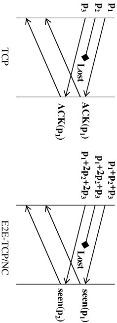
In order to combine the benefits of TCP and network coding, [11] proposes a new protocol called TCP/NC. The key idea is a new network coding layer between the transport layer and the network layer, which incurs minimal changes to the protocol stack. TCP/NC modifies TCP’s acknowledgement (ACK) scheme such that it acknowledges degrees of freedom instead of individual packets, as shown in Figure 1. This is done so by using the concept of “seen” packets – in which the number of degrees of freedom received is translated to the number of consecutive packets received. In [11], the authors present two versions of TCP/NC – one that adheres to the end-to-end philosophy of TCP, in which encoding and decoding operations are only performed at the source and destination, and another one that takes advantage of network coding even further by allowing any subset of intermediate nodes to re-encode. Note that re-encoding at the intermediate nodes is an optional feature of TCP/NC, and is not required for TCP/NC to work.
In this paper, we shall focus on TCP as well as TCP/NC with end-to-end network coding, which we denote E2E-TCP/NC (or in short E2E), in lossy networks. We adopt the same TCP model as in [2] – i.e. we consider standard TCP with Go-Back-N pipelining. Thus, the standard TCP discards packets that are out-of-order. We analytically show the throughput gains of E2E over standard TCP, and present simulations results that support this analysis. We develop upon the model introduced in [2] to characterize the steady state throughput behavior of both TCP and E2E as a function of erasure rate, round-trip time (RTT), and maximum window size. Our work thus extends the work of [2] for E2E-TCP/NC in lossy wireless networks. Furthermore, we use NS-2 (Network Simulator [12]) to verify our analytical results for TCP and E2E. Our analysis and simulations show that E2E is robust against erasures and failures. E2E is not only able to increase its window size faster but also maintain a large window size despite losses within the network. Thus, E2E is well suited for reliable communication in lossy networks. In contrast, standard TCP experiences window closing as losses are mistaken to be congestion.
The paper is organized as follows. In Section II, we introduce our communication model. In Section III, we briefly provide the intuition behind the benefit of using network coding with TCP. Then, we provide throughput analysis for TCP and E2E in Sections IV and V, respectively. In Section VI, we discuss the throughput behavior when the network is experiencing severe congestion, deep fading, and/or adversarial jamming. In Section VII, we provide simulation results to verify our analytical results in Sections IV and V. Finally, we conclude in Section VIII.
II A Model for TCP Congestion Control
We focus on TCP’s congestion avoidance mechanism, where the congestion control window size is incremented by each time an ACK is received. Thus, when every packet in the congestion control window is ACKed, the window size is increased to . On the other hand, the window size is reduced whenever an erasure/congestion is detected.
We model TCP’s behavior in terms of rounds as in [2]. We denote to be the size of TCP’s congestion control window size at the beginning of round . The sender transmit packets in its congestion window at the start of round , and once all packets have been sent, it defers transmitting any other packets until at least one ACK for the packets are received. The ACK reception ends the current round, and starts round .
For simplicity, we assume that the duration of each round is equal to a round trip time (), independent of . This assumes that the time needed to transmit a packet is much smaller than the round trip time. This implies the following sequence of events for each round : first, packets are transmitted. Some packets may be lost. The receiver transmits ACKs for the received packets. (Note that TCP uses cumulative ACKs. Therefore, if the packets arrive at the receiver in sequence, then the receiver ACKs packets . This signals that it has not yet received packet 4.) Some of the ACKs may also be lost. Once the sender receives the ACKs, it updates its window size. Assume that packets are acknowledged in round . Then, .
TCP reduces the window size for congestion control using the following two methods.
- 1.
Triple-duplicate (TD): When the TCP sender receives four ACKs with the same sequence number, then .
- 2.
Time-out (TO): If the Sender does not hear from the receiver for a predefined time period, called the “time-out” period (which is rounds long), then the sender closes its transmission window, . At this point, the sender updates its TO period to rounds, and transmits one packet. For any subsequent TO events, the sender transmits the one packet within its window, and doubles its TO period until is reached, after which the time-out period is fixed to . Once the sender receives an ACK from the receiver, it resets its TO period to and increments its window according to the congestion avoidance mechanism. During time-out, the throughput of both TCP and E2E is zero.
Finally, we note that in practice, the TCP receiver sends a single cumulative ACK after receiving number of packets, where typically. However, we assume that for simplicity. Extending the analysis to is straightforward.
II-A Maximum window size
In general, TCP cannot increase its window size unboundedly; there is a maximum window size . The TCP sender uses a congestion avoidance mechanism to increment the window size until , at which the window size remains until a TD or a TO event.
II-B Erasures
We assume that there are two different states: up-state and down-state. The network is in down-state when the network fails and the sender times-out. This may occur due to severe congestion, adversarial jamming, interference and deep fading, which are especially relevant for wireless networks. We denote to be the probability that the network is in the down-state during any given round. Note that during down-state, both TCP and E2E-TCP/NC have throughput of zero, as the forward and/or the backward paths have failed.
Assuming that the network is in up-state, we denote to be the probability that a packet is lost at any given time. We further assume that packet losses are independent. We note that this erasure model is different from that of [2] where losses are correlated within a round – i.e. bursty erasures. Correlated erasures model well bursty traffic and congestion in wireline networks. In our case, however, we are aiming to model wireless networks, thus we shall use random independent erasures.
II-C Performance metric


We analyze the performance of TCP and E2E in terms of two metrics: the average throughput , and the expected window evolution , where represents the total average throughput while window evolution reflects the perceived throughput at a given time. We define to be the number of packets received by the receiver during the interval . The total average throughput is defined as:
| (1) |
We denote and to be the average throughput for TCP and E2E, respectively.
III Intuition
For traditional TCP, erasures in the network can lead to triple-duplicate ACKs. For example, in Figure 2a, the sender transmits packets in round ; however, only of them arrive at the receiver. As a result, the receiver ACKs the packets and waits for packet . When the sender receives the ACKs, round starts. The sender updates its window (), and starts transmitting the new packets in the window. However, since the receiver is still waiting for packet , any other packets cause the receiver to request for packet . This results in a triple-duplicate ACKs event and the TCP sender closes its window, i.e. .
Notice that this window closing due to TD does not occur when using E2E as illustrated in Figure 2b. This is due to the fact that, with network coding, any linearly independent packet delivers new information. Thus, any subsequent packet (in Figure 2b, the first packet sent in round ) can be viewed as packet . As a result, the receiver is able to increment its ACK and the sender continues transmitting data.
It follows that network coding masks the losses within the network from TCP, and prevents it from closing its window by misjudging link losses as congestion. It is important to note that network coding translates losses as longer RTT, thus slowing down the transmission rate to adjust for losses without closing down the window in a drastic fashion.
IV Throughput Analysis for TCP
In this section, we consider the effect of losses for TCP. The throughput analysis for TCP is similar to that of [2]. However, the model has been modified from that of [2] to account for independent erasures and allow a fair comparison with network coded TCP. Assuming that the network is in its up-state, TCP can experience a TD or a TO event. As in [2], we first consider TD events, and then incorporate TO events.
We note that, despite independent packet erasures, a single packet loss may affect subsequent packet reception. This is due to the fact that TCP requires in-order reception. Thus, a single packet loss within a transmission window forces all subsequent packets in the window to be out of order. Thus, they are discarded by the TCP receiver. As a result, standard TCP’s throughput behavior with independent losses is similar to that of [2], where losses are correlated within one round.

IV-A Triple-duplicate for TCP
We consider the expected throughput between consecutive TD events, as shown in Figure 3. Assume that the TD events occurred at time and , . Assume that round begins immediately after time , and that packet loss occurs in the -th round, i.e. round .
First, we calculate . Note that during the interval , there are no packet losses. Given that the probability of a packet loss is , the expected number of consecutive packets that are successfully sent from sender to receiver is
| (2) |
The packets (in white in Figure 3) sent after the lost packets (in black in Figure 3) are out of order, and will not be accepted by the standard TCP receiver. Thus, Equation (2) does not take into account the packets sent in round or .
We calculate the expected time period between two TD events, . As in Figure 3, after the packet losses in round , there is an additional round for the loss feedback from the receiver to reach the sender. Therefore, there are rounds within the time interval , and . Thus,
| (3) |
To derive , note that and
| (4) |
Equation (4) is due to TCP’s congestion control. TCP interprets the losses in round as congestion, and as a result halves its window. Assuming that, in the long run, and that is uniformly distributed between ,
| (5) |
During these rounds, we expect to successfully transmit packets as noted in Equation (2). This results in the following equations:
| (6) | ||||
| (7) |
Taking the expectation of Equation (7) and using Equation (5),
| (8) |
Note that is assumed to be uniformly distributed across . Thus, by Equation (5). Solving Equation (8) for , we get the following:
| (9) |
This provides an expression of steady state average window size for TCP (using Equations (5) and (9)):
| (10) | ||||
| (11) |
The average throughput can be expressed as
| (12) |
For small , ; for large , . If we only consider TD events, the long-term steady state throughput is equal to that in Equation (12).
The analysis above assumes that the window size can grow unboundedly; however, this is not the case. To take maximum window size into account, we make a following approximation:
| (13) |
For small , this result coincide with the results in [2].
IV-B Time-out for TCP
We note that even when the network is in the up-state, TCP can experience TO events. This happens when enough loss events occur within two consecutive rounds such that there are only two or fewer out of order packets and all others are lost, as shown in Figure 3. Thus, , the probability of a TO event given a window size of , is given by
| (14) |
| (15) | ||||
| (16) |
| (17) |
We approximate in above Equation (14) with the expected window size from Equation (11). The length of the TO event depends on the duration of the loss events. Thus, the expected duration of TO period (in RTTs) is given in Equation (16). Finally, by combining the results in Equations (13), (14), and (16), we get an expression for the average throughput of TCP as shown in Equation (17).
V Throughput Analysis for E2E-TCP/NC
We consider the expected throughput for E2E given that the network is in up-state. It is important to note that erasure patterns that result in TD and/or TO events under TCP may not yield the same result under E2E, as illustrated in Section III. We emphasize again that this is due to the fact that any linearly independent packet conveys a new degree of freedom to the receiver. Figure 4 illustrates this effect – packets (in white) sent after the lost packets (in black) are acknowledged by the receivers, thus allowing E2E to advance its window.
This implies that E2E does not experience window closing often during the network up-state. We shall show that the window size is actually a non-decreasing function in . However, not surprisingly, the rate at which grows depends on as we shall show in the subsequent sections.

V-A E2E-TCP/NC Window Evolution

From Figure 4, we observe that E2E-TCP/NC is able to maintain its window size despite experiencing losses. Furthermore, E2E is able to receive packets that would be considered out of order by TCP. Consequently, E2E can avoid closing its window due to erasures. This is because every packet that is linearly independent of previously received packets is considered to be “innovative” and is therefore acknowledged. As a result, E2E’s window evolves differently from that of TCP, and can be characterized by a simple recursive relationship as
| (18) |
Note that the expected number of packets received in round , . Once we take the maximum window size into account, we have the following expression for E2E’s expected window size:
| (19) |
where is the round number. is the initial window size, and we set . Figure 5 shows an example of the evolution of the E2E window using Equation (19).
V-A1 Markov Chain Model

The above analysis describes the expected behavior of E2E’s window size. We can also describe the window size behavior using a Markov chain as shown in Figure 6. The states of this Markov chain represent the instantaneous window size (not specific to a round). A transition occurs whenever a packet is sent. We denote to be the state representing the window size of . Assume that we are at state . If a transmitted packet is received by the E2E receiver and acknowledged, the window is incremented by ; thus, we end up in state . Note that this occurs with probability . On the other hand, if the packet is lost, then the window stays at . This occurs with probability . Thus, the Markov chain states represent the window size, and the transitions correspond to packet transmissions.
Note that is an absorbing state of the Markov chain. As noted in Section III, E2E does not often experience a window shutdown, which implies that the network is in down-state. Thus, during the network up-state, E2E’s window size is a non-decreasing, as shown in Figure 6. Therefore, given enough time, we will reach state with probability equal to 1. Thus, we analyze the expected number of packet transmissions needed for absorption.
The transition matrix and the fundamental matrix of the Markov chain is given in Figure 7. The entry represents the expected number of visits to state before absorption – i.e. we reach state – when we start from state . Our objective is to find the expected number of packets transmitted to reach starting from state where . Thus, the partial sum of the first row entries of gives the expected number of packets transmitted until we reach the window size . The expression for the first row of can be derived using cofactors:
| (20) |
Therefore, the expected number of packet transmissions to reach a window size of is:
| (21) | ||||
| (22) |
Equation (22) is due to the fact that there are states before state .
Note that is equal to the area under the curve for rounds in Figure 5. This corresponds to the sum of (i.e. the number of packets transmitted every round) as it increases from to .
V-B E2E-TCP/NC Throughput Analysis per Round
Using the results in Section V-A, we derive an expression for the throughput. Once we have the expected value of the window size for any given round , the throughput is straight forward. The throughput of round , is directly proportional to the window size , i.e.
| (23) |
where is the redundancy factor of E2E-TCP/NC, and is the “effective” round trip time. We shall formally define and discuss the effect of and in the subsequent subsections.
We note that . At any given round , we expect to see packets transmitted by the E2E sender, and we expect packets to be lost. Thus, the E2E receiver can only acknowledge packets (or degrees of freedom), which results in the sender incrementing its window by . Thus, coincides with our intuition.
V-B1 Redundancy Factor
The redundancy factor is the ratio between the average rate at which linear combinations are sent to the receiver and the rate at which TCP’s window progresses. For example, if the sender has 10 packets in its window, then TCP/NC transmits linear combinations, unlike TCP which would send just 10 packets. This redundancy is necessary to (a) compensate for the losses within the network, and (b) match TCP’s sending rate to the rate at which data is actually received at the receiver. References [11][13] introduce the redundancy factor with TCP/NC, and show that the optimal value is .
It is important to discuss the effect of in the throughput. As noted in Equation (23), the throughput is inversely proportional to the redundancy factor . For example, for every 10 coded packets transmitted, there are only original data packets from the source. Thus, given any number of coded packets transmitted by the sender, the receiver only needs -fraction of them and the rest -fraction of the packets are redundant. Therefore, the throughput at any given round is inversely proportional to the redundancy factor. Specifically, .
The redundancy factor should be chosen with some care. By Equation (23), it may seem that setting would maximize throughput. However, setting causes significant performance degradation, since network coding can no longer fully compensate for the losses which may lead to window closing for E2E. To maximize throughput, an optimal value of should be chosen. However, need not be set to the optimal value for E2E-TCP/NC to work. Setting means that network coding may over-compensate for the losses within the network; thus, introducing more redundant packets than necessary. Thus, we assume that .
V-B2 Effective Round Trip Time
is the round trip time estimate that TCP maintains by sampling the behavior of packets sent over the connection. It is denoted because it is often referred to as “smoothed” round trip time as it is obtained by averaging the time for a packet to be acknowledged after the packet has been sent. We note that, in Equation (23), we use instead of because is the “effective” round trip time E2E experiences.
For E2E operating in lossy networks, is often greater than . This can be seen in Figure 1. The first coded packet () is received and acknowledged (). Thus, the sender is able to estimate the round trip time correctly; resulting in . However, the second coded packet () is lost. As a result, the third packet () is used to acknowledge the second degree of freedom (). We note that in our model, we assume for simplicity that the time needed to transmit a packet is much smaller than RTT (Section II); thus, despite the losses, our model would result in . However, in practice, depending on the size of the packets, the transmission time may not be negligible. This results in a longer round trip time estimate, which can be characterized as described below.
We define to be the time to transmit a packet. Then, the sender expects to receive an ACK of a packet after time units, where
| (24) | ||||
| (25) |
For simplicity, Equation (25) does not take into account the “edge effect” of packets that are waiting to be acknowledged across rounds. As the window size grows, the edge effect can safely be ignored.
V-C E2E-TCP/NC Average Throughput
Taking Equation (23), we can average the throughput over rounds to obtain the average throughput for E2E-TCP/NC.
| (26) | ||||
| (27) | ||||
| (28) |
where
Note that as , the average throughput .
VI Network in down-state
In this section, we consider the effect of , the probability of network being in down-state at any given round, during which the sender is unable to transfer data to the receiver (for both TCP and E2E). Note that the average throughput analysis in Sections IV and V gives the throughput during when the network is in up-state. Thus, the average throughput would depend on 1) the average number of rounds during the network up-state , and 2) the average length of down-state periods .


The average number of rounds during a network upstate is . The average length of down-state period is .
Taking into account both TD and TO events, the average throughput of TCP and E2E can be summarized as below. The long term average throughput of TCP is given in Equation (29). The long term average throughput of E2E is given in Equation (30). As discussed in Section V-C, depends on the number of rounds ; thus, the length of affects its performance.
| (29) | ||||
| (30) | ||||
| (31) |
VII Simulation results
In this section, we use simulations to verify that our analysis captures the behavior of both TCP and E2E. We use NS-2 (Network Simulator [12]) to simulate TCP and E2E-TCP/NC where TCP-Vegas is used as the underlying TCP protocol. We use the implementation of E2E from [13]. The network topology for the simulation is shown in Figure 9. All links, in both forward and backward paths, are assumed to have a bandwidth of 1 Mbps, a propagation delay of 100 ms, a buffer size of 200, and a erasure rate of . Each packet transmitted is assumed to be 8000 bits (1000 bytes). We set packets for all simulations. We fix the redundancy factor for all . We note that the optimal redundancy factor varies with . In addition, time-out period rounds long (3 seconds).


To compare the performance of TCP and E2E, we average the performance over 30 independent runs of the simulation, each of which is 1000 seconds long. We vary the per link probability of erasure, . We consider , 0.025, and . Note that since there are in total four links in the path from node 0 to node 4, the probability of packet erasure is . Therefore, the corresponding values are 0.0587, 0.0963, and 0.1855.
First, we show the throughput benefits of E2E over TCP in Figure 10. As our analysis predicts, E2E sustains its high throughput despite the erasures present in the network. We observe that TCP may close its window due to triple-duplicates ACKs; however, E2E is more resilient to such erasure patterns. Therefore, E2E is able to increment its window consistently even with erasures and achieve a window size of sooner than that of TCP. In Figure 10b, we observe that E2E converges to very rapidly for , and 0.025. More importantly, E2E is able to maintain the window size of 90 even under lossy conditions when standard TCP is unable to (resulting in the window fluctuation in Figure 10b).
We note that for , the throughput behavior is not as steady. This is due to the increase in loss rate, i.e. . Given that and link capacities 1 Mbps, the effective maximum throughput we can achieve is Mbps. Since each packet is 8000 bits and RTT = 0.8 seconds, we can expect the throughput to be at most packets per second, which is less than . As a result, the bottleneck is not but the link capacity for . This is consistent with the performance we see in Figure 10b.

An interesting observation is that, TCP achieves a moderate average window size (depending on , 20-60 packets) while E2E achieves average window size of 90 (where ). However, the average throughput of E2E is much higher than that of TCP’s, as shown in Figure 10a and Table I. This is because, before closing its window (TD or TO event), the TCP sender waits for a certain period of time, called retransmission timeout period. This retransmission timeout period is approximately set to . During this retransmission timeout period, the TCP sender maintains its window size, despite the fact that it is idle and waiting for acknowledgements. Thus, for TCP, the average window size may be much larger than the average throughput. On the other hand, E2E does not experience TD or TO events as often; thus, the window size commensurate the average throughput. Although we did not explicitly take retransmission timeout into consideration in the TCP analysis in Section IV, the retransmission timeout is not difficult to incorporate. For every TD or TO event, TCP idles for two extra round-trip time, which can be incorporated by letting and .


As described in Sections III and V-B2, E2E masks errors by translating losses as longer RTT. For E2E, if a specific packet is lost, the next subsequent packet received can “replace” the lost packet; thus, allowing the receiver to send an ACK. Therefore, the longer RTT estimate takes into account the delay associated with waiting for the next subsequent packet at the receiver. In Figure 11 and Table I, we verify that this is indeed true. In the simulation, we have a round trip time of ms. TCP, depending on the ACKs received, modifies its RTT estimation; thus, due to random erasures, TCP’s RTT estimate fluctuates significantly. On the other hand, E2E is able to maintain a consistent estimate of the RTT; however, is slightly above the actual 800 ms.
| Average E2E SRTT | E2E simulation | E2E analysis () | TCP simulation | TCP analysis | ||
|---|---|---|---|---|---|---|
| 0.015 | 0.0587 | 0.8396 | 0.6242 | 0.6202 | 0.0264 | 0.0231 |
| 0.025 | 0.0963 | 0.8434 | 0.6161 | 0.5917 | 0.0136 | 0.0150 |
| 0.05 | 0.1855 | 0.8540 | 0.5200 | 0.5243 | 0.0067 | 0.0065 |
Finally, we examine the accuracy of our analytical model in predicting the behavior of TCP and E2E. First, note that our analytical model of window evolution (shown in Equation (19) and Figure 5) demonstrates the same trend as that of the window evolution of E2E NS-2 simulations (shown in Figure 10b). Second, we compare the actual NS-2 simulation performance to the analytical model. This is shown in Figure 12 and Table I. From the results, we observe that Equations (23) and (19) predict well the trend of E2E’s throughput and window evolution, and provides a good estimate of E2E’s performance. Furthermore, our analysis predicts the average TCP behavior very well. In Figure 12 and Table I, we see that Equation (17) is consistent with the NS-2 simulation results even for large values of . Therefore, both simulations as well as analysis support that E2E is resilient to erasures; thus, better suited for reliable transmission over unreliable networks, such as wireless networks.
VIII Conclusions
We have presented an analytical study and compared the performance of TCP and E2E-TCP/NC. Our analysis characterizes the throughput of TCP and E2E as a function of erasure rate, round-trip time, maximum window size, and duration of the connection. We showed that network coding, which is robust against erasures and failures, can prevent TCP’s performance degradation often observed in lossy networks. Our analytical model shows that TCP with network coding has significant throughput gains over TCP. E2E is not only able to increase its window size faster but also to maintain a large window size despite losses within the network; on the other hand, TCP experiences window closing as losses are mistaken to be congestion. Furthermore, NS-2 simulations verify our analysis on TCP’s and E2E’s performance. Our analysis and simulation results both support that E2E is robust against erasures and failures. Thus, E2E is well suited for reliable communication in lossy wireless networks.
References
- [1] R. Cáceres and L. Iftode, “Improving the performance of reliable transport protocols in mobile computing environments,” IEEE Journal on Selected Areas in Communications, vol. 13, no. 5, June 1995.
- [2] J. Padhye, V. Firoiu, D. Towsley, and J. Kurose, “Modeling TCP throughput: A simple model and its empirical validation,” in Proceedings of the ACM SIGCOMM, 1998.
- [3] H. Balakrishnan, V. N. Padmanabhan, S. Seshan, and R. H. Katz, “A comparison of mechanisms for improving tcp performance over wireless links,” IEEE/ACM Transactions on Networking, vol. 5.
- [4] Y. Tian, K. Xu, and N. Ansari, “TCP in wireless environments: Problems and solutions,” IEEE Comm. Magazine, vol. 43, pp. 27–32, 2005.
- [5] R. Ahlswede, N. Cai, S.-Y. R. Li, and R. W. Yeung, “Network information flow,” IEEE Transactions on Information Theory, vol. 46, pp. 1204–1216, 2000.
- [6] R. Koetter and M. Médard, “An algebraic approach to network coding,” IEEE/ACM Transaction on Networking, vol. 11, pp. 782–795, 2003.
- [7] S. Katti, H. Rahul, W. Hu, D. Katabi, M. Médard, and J. Crowcroft, “Xors in the air: Practical wireless network coding,” in Proceedings of ACM SIGCOMM, 2006.
- [8] S. Chachulski, M. Jennings, S. Katti, and D. Katabi, “Trading structure for randomness in wireless opportunistic routing,” in Proceedings of ACM SIGCOMM, 2007.
- [9] B. L. Yunfeng Lin, Baochun Li, “CodeOr: Opportunisitic routing in wireless mesh networks with segmented network coding,” in Proceedings of IEEE International Conference on Network Protocols, 2008.
- [10] J. Barros, R. A. Costa, D. Munaretto, and J. Widmer, “Effective delay control for online network coding,” in Proceedings of IEEE INFOCOM, 2009.
- [11] J. K. Sundararajan, D. Shah, M. Médard, M. Mitzenmacher, and J. Barros, “Network coding meets TCP,” in Proceedings of IEEE INFOCOM, April 2009, pp. 280–288.
- [12] “Network simulator (ns-2),” http://www.isi.edu/nsnam/ns/.
- [13] J. K. Sundararajan, S. Jakubczak, M. Médard, M. Mitzenmacher, and J. Barros, “Interfacing network coding with tcp: an implementation,” Tech. Rep., August 2009, http://arxiv.org/abs/0908.1564.