A diagrammatic treatment of neutrino oscillations

The neutrino-oscillation hypothesis suggested by Bruno Pontecorvo [1] offers the most probable and promising explanation of the anomalies discovered in many experiments with solar, atmospheric, reactor and accelerator neutrinos and antineutrinos. However the conventional quantum-mechanical (QM) theory of neutrino oscillations faces a number of methodological difficulties and paradoxes which have been widely discussed by many authors (see, e.g., [3, 4, 5, 6, 7, 8, 9] and numerous references therein). It has been recognized that, remaining within the framework of quantum mechanics, some problems of the conventional theory can be resolved by using wave packets to describe the neutrino states and/or the states of the particles involved in the processes of neutrino production and detection. In this way it has been found, e.g., that neutrino oscillations vanish if the neutrinos propagate over the distances much larger than the coherence length (for in-depth discussion, see [7]).

A more radical approach to the problem is based on quantum field theory (QFT) [10, 11, 15, 16, 17]; see also [7, 8, 9] for further references. In this approach, the sequential processes of neutrino production and detection are treated as a single process which can be described by the $S$-matrix formalism of QFT. The peculiarity (or better to say novelty) of this approach is in the use of Feynman diagrams with vertices separated by macroscopically large spacetime intervals. Besides, as in the QM case, for the description of the asymptotically free “in” and “out” states one has to use wave packets rather than the ordinary (in QFT) Fock states with definite 4-momenta. In this framework, the neutrinos appear as the propagators of the neutrino mass eigenfields, $\nu_{i}$, connecting the macroscopically distant parts of the Feynman diagram. In the new approach, there is no need in even mentioning the flavor neutrino states or fields, and the neutrino oscillation phenomenon is a reflection of the usual interference of the Feynman diagrams with different $\nu_{i}$’s in the intermediate states. Such treatment not only enables us to reproduce the standard QM formula for the flavor transition probability and obtain the pertinent QFT corrections (thus offering a potential possibility for an experimental verification of the theory) but also impels us to re-examine the concept of neutrino flavor mixing.

The authors of the mentioned pioneer papers do use (explicitly or implicitly) the noncovariant, usually Gaussian wave packets, which are only applicable, as it will be shown in the next section, to nonrelativistic particles. However, in the reactions of neutrino production and detection taking part in the current neutrino oscillation experiments, relativistic particles are as a rule involved.¹¹ 1 An important exception from the rule might be experiments with Mössbauer antineutrinos which are under active discussion in the current literature  [20, 22, 24, 26, 27]. Moreover, by an appropriate Lorentz boost, any particle can be made to be ultrarelativistic. Therefore it is necessary to work out a relativistically covariant (inertial frame-independent) theory of wave packets applicable for the description of particles with arbitrary momenta.

In this paper we propose a simple covariant wave-packet theory (section 2), which is then applied to the calculation of the interference of macroscopic diagrams with massive neutrino exchange (section 4). We perform a statistical averaging of the probability (the squared absolute value of the overall amplitude) which leads to a rather general formula for the neutrino event rate in the detector (section 5); the conditions of applicability of the conventional QM formula for the flavor transition probability are also discussed. In section 6 we summarise the main results of the formalism.

We will deal with the Feynman diagrams, the generic structure of which is shown in figure 3.

The external legs of such diagrams correspond to asymptotically free incoming (“in”) and outgoing (“out”) wave packets in the coordinate representation, that is, to the wavefunctions $\psi_{a}\left(\boldsymbol{p}_{a},x_{a}\right)$ and $\psi_{b}^{*}\left(\boldsymbol{p}_{b},x_{b}\right)$ specified by the most probable momenta $\boldsymbol{p}_{a,b}$, spacetime coordinates $x_{a,b}$, masses $m_{a,b}$ and parameters $\sigma_{a,b}$. Here and below we use the following notation: $I_{s}$ ($F_{s}$) is the set of in (out) packets in the block $X_{s}$ (“source”), $I_{d}$ ($F_{d}$) is the set of in (out) packets in the block $X_{d}$ (“detector”). The internal line connecting the blocks $X_{s}$ and $X_{d}$ denotes the causal Green’s function of the neutrino mass eigenfield $\nu_{i}$ ($i=1,2,3$). The blocks $X_{s}$ and $X_{d}$ are assumed to be macroscopically separated in spacetime; this explains the term “macroscopic diagram”.

In the calculations with the macrodiagrams of such kind, we will encounter the four-dimensional overlap integrals $\mathbb{V}_{s}(q)$ and $\mathbb{V}_{d}(q)$ defined as follows:

$\displaystyle\mathbb{V}_{s,d}(q)=\int dxe^{\pm iqx}\Big[\prod_{a\in{I_{s,d}}}e^{-ip_{a}x_{a}}\psi_{a}\left(\boldsymbol{p}_{a},x_{a}-x\right)\Big]\Big[\prod_{b\in{F_{s,d}}}e^{ip_{b}x_{b}}\psi_{b}^{*}\left(\boldsymbol{p}_{b},x_{b}-x\right)\Big].$

In the CRGP approximation, these integrals can be written in the form

$\displaystyle\mathbb{V}_{s,d}(q)=\int dx\exp\Big[i\left(\pm qx-q_{s,d}x\right)-\sum_{\varkappa{\in}S,D}T_{\varkappa}^{\mu\nu}\left(x_{\varkappa}-x\right)_{\mu}\left(x_{\varkappa}-x\right)_{\nu}\Big],$

(25)

where

$\displaystyle q_{s}=\sum_{a\in{I_{s}}}p_{a}-\sum_{b\in{F_{s}}}p_{b},\qquad q_{d}=\sum_{a\in{I_{d}}}p_{a}-\sum_{b\in{F_{d}}}p_{b},$

$\displaystyle T_{\varkappa}^{\mu\nu}=\sigma_{\varkappa}^{2}\left(u_{\varkappa}^{\mu}u_{\varkappa}^{\nu}-g^{\mu\nu}\right),\qquad S=I_{s}{\oplus}F_{s},\qquad D=I_{d}{\oplus}F_{d},$

$u_{\varkappa}=p_{\varkappa}/m_{\varkappa}=\Gamma_{\varkappa}(1,\boldsymbol{v}_{\varkappa})$ is the 4-velocity of packet $\varkappa$ ($\varkappa=a,b$) and, finally, $q$ is the 4-momentum of the virtual neutrino. Let us now define the symmetric overlap tensors for the source and detector:

$\displaystyle\Re_{s}^{\mu\nu}=\sum_{\varkappa{\in}S}T_{\varkappa}^{\mu\nu}\qquad\mathrm{and}\qquad\Re_{d}^{\mu\nu}=\sum_{\varkappa{\in}D}T_{\varkappa}^{\mu\nu}.$

One can prove that these tensors are positive definite provided $\sigma_{\varkappa}\neq 0$ ($\forall\varkappa$); thus, there exist the positive-definite tensors $\widetilde{\Re}_{s}^{\mu\nu}$ and $\widetilde{\Re}_{d}^{\mu\nu}$ such that $\widetilde{\Re}_{s,d}^{\mu\lambda}\left(\Re_{s,d}\right)_{\lambda\nu}=\delta^{\mu}_{\nu}$ or, in the matrix form, $\widetilde{\Re}_{s,d}=||\widetilde{\Re}_{s,d}^{\mu\nu}||=g\,\Re_{s,d}^{-1}\,g$, where $\Re_{s,d}=||\Re_{s,d}^{\mu\nu}||$ and $g=||g_{\mu\nu}||$. Obviously, $|\Re_{s,d}|>0$ and $|\widetilde{\Re}_{s,d}|=|\Re_{s,d}|^{-1}$. These facts allow us to compute the integrals (25) explicitly. For this aim, we define the quantities

	$\displaystyle\widetilde{\delta}_{s,d}(K)=(4\pi)^{-2}|\Re_{s,d}|^{-1/2}\exp\left(-\frac{1}{4}\widetilde{\Re}_{s,d}^{\mu\nu}K_{\mu}K_{\nu}\right),$		(26)
	$\displaystyle X_{s,d}^{\mu}=\widetilde{\Re}_{s,d}^{\mu\nu}\,\sum_{\varkappa}T_{\varkappa\nu}^{\lambda}x_{\varkappa\lambda}=\widetilde{\Re}_{s,d}^{\mu\nu}\,\sum_{\varkappa}\sigma_{\varkappa}^{2}\left[(u_{\varkappa}x_{\varkappa})u_{\varkappa\nu}-x_{\varkappa\nu}\right],$		(27)
	$\displaystyle\mathfrak{S}_{s,d}=\sum_{\varkappa,\varkappa^{\prime}}\left(\delta_{\varkappa\varkappa^{\prime}}T_{\varkappa}^{\mu\nu}-T_{\varkappa\mu^{\prime}}^{\mu}\,\widetilde{\Re}_{s,d}^{\mu^{\prime}\nu^{\prime}}\,T_{\varkappa^{\prime}\nu^{\prime}}^{\nu}\right)x_{\varkappa\mu}x_{\varkappa^{\prime}\nu}$		(28)

(here $\varkappa,\varkappa^{\prime}{\in}S,D$ and $K$ is an arbitrary 4-momentum). With this notation, we find the following compact expression for the integral (25):

$\displaystyle\mathbb{V}_{s,d}(q)=(2\pi)^{4}\widetilde{\delta}_{s,d}\left(q{\mp}q_{s,d}\right)\exp\left[-\mathfrak{S}_{s,d}~{\pm}~i\left(q{\mp}q_{s,d}\right)X_{s,d}\right].$

Let us clarify the physical meaning of functions (26)–(28). In the plane-wave limit ($\sigma_{\varkappa}\to 0$) the factors $\widetilde{\delta}_{s}\left(q-q_{s}\right)$ and $\widetilde{\delta}_{d}\left(q+q_{d}\right)$ become usual $\delta$ functions responsible for the exact energy-momentum conservation in the source and detector vertices, whereas at nonzero $\sigma_{\varkappa}$, they only lead to an approximate energy-momentum conservation: the probability of the process $I_{s}{\oplus}I_{d}\to F_{s}{\oplus}F_{d}$ is strongly suppressed at a small disbalance in the 4-momenta of the interacting packets and the allowed disbalance is defined by the tensors $\widetilde{\Re}_{s}^{\mu\nu}$ and $\widetilde{\Re}_{d}^{\mu\nu}$, i.e., ultimately, by the momentum spreads of the packets.

The functions $\exp\left(-\mathfrak{S}_{s}\right)$ and $\exp\left(-\mathfrak{S}_{d}\right)$ are the geometric suppression factors conditioned by a partial overlap of the wave packets in the spacetime region of their interaction. This can be seen after converting (28) to the form³³ 3 In this derivation we have used the translation invariance of the functions $\mathfrak{S}_{s,d}$.

$\displaystyle\mathfrak{S}_{s,d}=\sum_{\varkappa}T_{\varkappa}^{\mu\nu}\left(x_{\varkappa}-X_{s,d}\right)_{\mu}\left(x_{\varkappa}-X_{s,d}\right)_{\nu}$

(29)

and taking into account that $\mathfrak{S}_{s,d}$ and $X_{s,d}$ are invariants under the group of transformations $x_{\varkappa}^{0}\longmapsto x_{\varkappa}^{0}+\tau_{\varkappa}$, $\boldsymbol{x}_{\varkappa}\longmapsto\boldsymbol{x}_{\varkappa}+\boldsymbol{v}_{\varkappa}\tau_{\varkappa}$ with arbitrary real parameters $\tau_{\varkappa}$. The latter symmetry allows, for each packet $\varkappa{\in}S,D$ having a nonzero velocity $\boldsymbol{v}_{\varkappa}$, the vector $\boldsymbol{x}_{\varkappa}$ in (29) to be replaced with the vector

$\displaystyle\boldsymbol{b}_{\varkappa}=\left(\boldsymbol{x}_{\varkappa}-\boldsymbol{X}_{s,d}\right)-\left[\boldsymbol{n}_{\varkappa}\left(\boldsymbol{x}_{\varkappa}-\boldsymbol{X}_{s,d}\right)\right]\boldsymbol{n}_{\varkappa}\qquad(\boldsymbol{n}_{\varkappa}=\boldsymbol{v}_{\varkappa}/|\boldsymbol{v}_{\varkappa}|)$

(30)

(whose absolute value, $|\boldsymbol{b}_{\varkappa}|=\left|\boldsymbol{n}_{\varkappa}\times\left(\boldsymbol{x}_{\varkappa}-\boldsymbol{X}_{s,d}\right)\right|$, is the minimum distance between the classical world line of the center of the packet $\varkappa$ and the point $\boldsymbol{X}_{s,d}$), and the zero component $x_{\varkappa}^{0}$ to be replaced with the time $b_{\varkappa}^{0}$ of maximum approach of the packet center to the point $\boldsymbol{X}_{s,d}$, this time being equal to

$\displaystyle b_{\varkappa}^{0}=\left(x_{\varkappa}^{0}-X^{0}_{s,d}\right)-|\boldsymbol{v}_{\varkappa}|^{-1}\boldsymbol{n}_{\varkappa}\left(\boldsymbol{x}_{\varkappa}-\boldsymbol{X}_{s,d}\right).$

(31)

The 4-vector $b_{\varkappa}=(b_{\varkappa}^{0},\boldsymbol{b}_{\varkappa})$, built from (30) and (31), is a relativistic analog of the usual impact parameter, so it is natural to call it the impact vector. The 4-vectors $X_{s}$ and $X_{d}$ can be called, accordingly, the impact points. If $\boldsymbol{v}_{\varkappa}\neq 0$ ($\forall\varkappa$) then, after the substitution $x_{\varkappa}~\longmapsto~b_{\varkappa}$, the expression (29) becomes

$\displaystyle\mathfrak{S}_{s,d}=\sum_{\varkappa}\sigma_{\varkappa}^{2}\left[\left(\Gamma_{\varkappa}^{2}-1\right)\left(b^{0}_{\varkappa}\right)^{2}+\boldsymbol{b}_{\varkappa}^{2}\right]=\sum_{\varkappa}\sigma_{\varkappa}^{2}|\boldsymbol{b}_{\varkappa}^{\star}|^{2}.$

In the last equality, the contribution from each packet is written in its own rest frame (in which $|\boldsymbol{b}_{\varkappa}^{\star}|=|\boldsymbol{x}_{\varkappa}^{\star}-\boldsymbol{X}_{s,d}^{\star}|$), and hence the temporal limitation $\boldsymbol{v}_{\varkappa}\neq 0$ can be bypassed. The physical meaning of the factors $\exp\left(-\mathfrak{S}_{s}\right)$ and $\exp\left(-\mathfrak{S}_{d}\right)$ is now transparent: the interaction of in and out packets is unsuppressed ($\mathfrak{S}_{s,d}\ll 1)$ if all impact parameters $|\boldsymbol{b}_{\varkappa}^{\star}|$ are small relative to the effective dimensions of the packets $\varkappa$ ($\sim 1/\sigma_{\varkappa}$). In the lab. frame, the suppression of “unlucky” configurations of the packets’ world lines are defined by both the space and time components of the impact vectors $b_{\varkappa}$. The contribution of the time components $b^{0}_{\varkappa}$ is less important for nonrelativistic packets (with $\Gamma_{\varkappa}\sim 1$), but is very essential for ultrarelativistic packets (with $\Gamma_{\varkappa}\gg 1$).

Our consideration suggests that the impact points $X_{s}$ and $X_{d}$ identify the spacetime position of the regions of effective interaction of the packets in the source and detector, respectively. The more intensive interaction of the packets, the closer their world lines are placed with respect to the impact points. The condition that the interaction regions in the source and detector are macroscopically separated is equivalent to the macroscopic separation of the impact points. The world line configurations and impact point coordinates have no concern with the dynamics governed by the interaction Lagrangian, being uniquely defined by the initial (final) coordinates, group velocities and effective dimensions of the asymptotically free in (out) packets. But, of course, the full probability of the process $I_{s}{\oplus}I_{d}\to F_{s}{\oplus}F_{d}$ is defined by both the suppression factors $\exp\left(-\mathfrak{S}_{s}\right)$ and $\exp\left(-\mathfrak{S}_{d}\right)$ and interaction dynamics.

It is evident now that the spacetime remoteness of the initial 4-coordinates of the in and out wave packets from the interaction region means simply that

	$\displaystyle x_{a}^{0}$	$\displaystyle\ll X_{s,d}^{0},\qquad\left|\boldsymbol{x}_{a}-\boldsymbol{X}_{s,d}\right|\gg{\max}_{a}\left(\sigma_{a}^{-1}\right),\qquad a{\in}I_{s,d},$
	$\displaystyle x_{b}^{0}$	$\displaystyle\gg X_{s,d}^{0},\qquad\left|\boldsymbol{x}_{b}-\boldsymbol{X}_{s,d}\right|\gg{\max}_{b}\left(\sigma_{b}^{-1}\right),\qquad b{\in}F_{s,d}.$

Therewith, for the applicability of the CRGP model it is necessary that the components $X_{s,d}^{\mu}-x_{\varkappa}^{\mu}$ remain finite in magnitude and satisfy the conditions (21). It is meaningful to note that the requirement of spatial remoteness is in fact unnecessary for specification of the asymptotically free initial and final states. Indeed, some of the packets (e.g. a target nucleus or decaying meson in the source vertex) can be at rest in the lab. frame and thus they must be spatially close to the corresponding impact point; otherwise, the resultant interaction amplitude will be strongly suppressed by the geometric factor $\exp\left(-\mathfrak{S}_{s}\right)$ or $\exp\left(-\mathfrak{S}_{d}\right)$.

As a practically important example, we consider the charged-current induced production of the charged leptons $\ell_{\alpha}^{+}$ and $\ell_{\beta}^{-}$ ($\ell_{\alpha,\beta}=e,\mu,\tau$) in the process

$\displaystyle I_{s}{\oplus}I_{d}\to F_{s}^{\prime}+\ell_{\alpha}^{+}~{\oplus}~F_{d}^{\prime}+\ell_{\beta}^{-}.$

(32)

We assume for definiteness that all the external substates $I_{s}$, $I_{d}$, $F_{s}^{\prime}$ and $F_{d}^{\prime}$ consist exclusively of (asymptotically free) hadronic wave packets. Consequently, if $\alpha\neq\beta$, the process (32) violates the lepton numbers $L_{\alpha}$ and $L_{\beta}$ that is only possible via exchange of massive neutrinos (no matter whether they are Dirac or Majorana particles). In the lowest nonvanishing order in electroweak interactions, the process (32) is described by the sum of diagrams of figure 4.

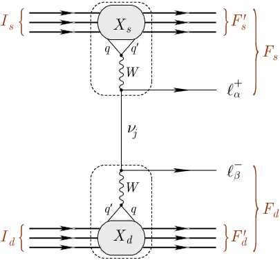
Let $X_{s}$ and $X_{d}$ be the impact points defined by eq. (27). We require these points and by that the effective regions of interactions in the source and detector (the areas symbolically outlined in figure 4 by dashed curves) to be macroscopically separated and the conditions

$\displaystyle x_{a}^{0}\ll X_{s,d}^{0}\quad(\forall a\in I_{s,d})\quad\mathrm{and}\quad x_{b}^{0}\gg X_{s,d}^{0}\quad(\forall b\in F_{s,d})$

to be fulfilled. Hence the incoming and outgoing states are thought to be direct products of free one-packet states (2), each normalized according to the relation (11).

In the framework of the standard model (SM) phenomenologically extended by inclusion of a neutrino mass term, the quark-lepton blocks of the diagram of figure 4 are described by the Lagrangian

$\displaystyle\mathcal{L}_{W}(x)=-\frac{g}{2\sqrt{2}}\left[j_{\ell}(x)W(x)+j_{q}(x)W(x)+\mathrm{H.c.}\right],$

where $g$ is the $SU(2)$ gauge coupling constant, $j_{\ell}$ and $j_{q}$ are the lepton and quark weak charged currents,

$\displaystyle j_{\ell}^{\mu}(x)=\sum_{{\alpha}i}V_{{\alpha}i}^{*}\,\overline{\nu}_{i}(x)O^{\mu}\ell_{\alpha}(x),\qquad j_{q}^{\mu}(x)=\sum_{qq^{\prime}}V_{qq^{\prime}}^{{}^{\prime}*}\,\overline{q}(x)O^{\mu}q^{\prime}(x),$

$V_{{\alpha}i}$ ($\alpha=e,\mu,\tau$, $i=1,2,3$) and $V^{\prime}_{qq^{\prime}}$ ($q=u,c,t$, $q^{\prime}=d,s,b$) are the elements of the neutrino and quark mixing matrices ($\boldsymbol{V}$ and $\boldsymbol{V}^{\prime}$, respectively), $\ell_{\alpha}(x)$ and $\ell_{\beta}(x)$ are the charged lepton fields, and $O^{\mu}=\gamma^{\mu}(1-\gamma_{5})$. The customary notation is used for other fields and Dirac $\gamma$-matrices. The normalized dimensionless amplitude of the process (32)

$\displaystyle\langle\mathrm{\bf out}|\mathbb{S}|\mathrm{\bf in}\rangle\left(\langle\mathrm{\bf in}|\mathrm{\bf in}\rangle\langle\mathrm{\bf out}|\mathrm{\bf out}\rangle\right)^{-1/2}~\stackrel{{\scriptstyle\mathrm{def}}}{{=}}~\mathcal{A}_{\beta\alpha}$

is given by the fourth order of the perturbation theory in the coupling constant $g$:

	$\displaystyle\mathcal{A}_{\beta\alpha}=\frac{1}{\mathcal{N}}\left(\frac{-ig}{2\sqrt{2}}\right)^{4}\langle F_{s}{\oplus}F_{d}|T\int dxdx^{\prime}dydy^{\prime}:j_{\ell}(x)W(x):\,:j_{q}(x^{\prime})W^{\dagger}(x^{\prime}):$		(33)
	$\displaystyle\times:j_{\ell}^{\dagger}(y)W^{\dagger}(y):\,:j_{q}^{\dagger}(y^{\prime})W(y^{\prime}):\mathbb{S}_{h}|I_{s}{\oplus}I_{d}\rangle.$		(34)

Here $\mathbb{S}_{h}=\exp\left[i\int dz\mathcal{L}_{\mathrm{h}}(z)\right]$, $\mathcal{L}_{\mathrm{h}}(z)$ is the Lagrangian of strong and electromagnetic interactions responsible for nonperturbative processes of fragmentation and hadronization; $T$ and $:\ldots:$ are the standard symbols for the chronological and normal ordering of local operators. The normalization factor $\mathcal{N}$ in the CRGP approximation is given by

$\displaystyle\mathcal{N}^{2}=\langle\mathrm{\bf in}|\mathrm{\bf in}\rangle\langle\mathrm{\bf out}|\mathrm{\bf out}\rangle=\prod_{\varkappa{\in}I_{s}{\oplus}I_{d}{\oplus}F_{s}{\oplus}F_{d}}2E_{\varkappa}\mathrm{V}_{\varkappa}(\boldsymbol{p}_{\varkappa}).$

(35)

The assumed narrowness of the wave packets in the momentum space, macroscopic remoteness of the interaction regions in the source and detector, and the consideration of translation invariance allow us to represent the hadronic part of the amplitude (33) in the factorized form

$\displaystyle\langle F_{s}^{\prime}{\oplus}F_{d}^{\prime}|T\left[:j_{q}^{\mu}(x):\,:j_{q}^{{\dagger}\nu}(y):\mathbb{S}_{h}\right]|I_{s}{\oplus}I_{d}\rangle=\mathcal{J}_{s}^{\mu}(p_{S})\mathcal{J}_{d}^{\nu*}(p_{D})\Pi^{\prime},$

	$\displaystyle\Pi^{\prime}=\Big[\prod_{a{\in}I_{s}}e^{-ip_{a}x_{a}}\psi_{a}(\boldsymbol{p}_{a},x_{a}-x)\Big]\Big[\prod_{b{\in}F_{s}^{\prime}}e^{ip_{b}x_{b}}\psi_{b}^{*}(\boldsymbol{p}_{b},x_{b}-x)\Big]$
	$\displaystyle\times\Big[\prod_{a{\in}I_{d}}e^{-ip_{a}x_{a}}\psi_{a}(\boldsymbol{p}_{a},x_{a}-y)\Big]\Big[\prod_{b{\in}F_{d}^{\prime}}e^{ip_{b}x_{b}}\psi_{b}^{*}(\boldsymbol{p}_{b},x_{b}-y)\Big],$

where $\mathcal{J}_{s}(p_{S})$ and $\mathcal{J}_{d}(p_{D})$ are the $c$-number hadronic currents in which the strong interactions are taken into account nonperturbatively, and $p_{S}$ and $p_{D}$ denote the sets of the momentum and spin variables of the hadronic states. Now, by applying Wick’s theorem and the known properties of the leptonic wave packets, the amplitude (33) can be rewritten in the following way:

$\displaystyle\mathcal{A}_{\beta\alpha}=\frac{g^{4}}{64\mathcal{N}}\sum_{j}V_{{\beta}j}\mathcal{J}_{d}^{\nu*}\overline{u}(\boldsymbol{p}_{\beta})O^{\nu^{\prime}}\mathbb{G}^{j}_{\nu\nu^{\prime}\mu^{\prime}\mu}\left(\{\boldsymbol{p}_{\varkappa},x_{\varkappa}\}\right)O^{\mu^{\prime}}v(\boldsymbol{p}_{\alpha})\mathcal{J}_{s}^{\mu}V^{*}_{{\alpha}j},$

(36)

where we have introduced the tensor function

$\displaystyle\mathbb{G}^{j}_{\nu\nu^{\prime}\mu^{\prime}\mu}\left(\{\boldsymbol{p}_{\varkappa},x_{\varkappa}\}\right)=\int\frac{dq}{(2\pi)^{4}}\mathbb{V}_{d}(q)\Delta_{\nu\nu^{\prime}}(q-p_{\beta})\Delta^{j}(q)\Delta_{\mu^{\prime}\mu}(q+p_{\alpha})\mathbb{V}_{s}(q).$

(37)

Here $\mathbb{V}_{s}(q)$ and $\mathbb{V}_{d}(q)$ are the overlap integrals discussed in detail in section 3,

$\displaystyle\Delta^{j}(q)=i\left(\hat{q}-m_{j}+i0\right)^{-1}$

and $\Delta_{\mu\nu}$ are the propagators of, respectively, the massive neutrino $\nu_{j}$ and $W$ boson (the explicit form of $\Delta_{\mu\nu}$ is not used below), $m_{j}$ and $m_{W}$ are their masses, $v(\boldsymbol{p}_{\alpha})$ and $\overline{u}(\boldsymbol{p}_{\beta})$ are the Dirac bispinors describing the leptons $\ell_{\alpha}^{+}$ and $\ell_{\beta}^{-}$, respectively. Here and below, the spin indices and arguments of the functions $\mathcal{J}_{s,d}$ are omitted for short.

References

- [1] Pontecorvo B 1957 “Mesonium and anti-mesonium”, Zh. Eksp. Teor. Fiz. 33 549 [Sov. Phys. JETP 6 429]
- [2] [] Pontecorvo B 1957 “Inverse beta processes and nonconservation of lepton charge”, Zh. Eksp. Teor. Fiz. 34 247 [Sov. Phys. JETP 7 172]
- [3] Kayser B 1981 “On the quantum mechanics of neutrino oscillation”, Phys. Rev. D 24 110
- [4] Giunti C, Kim C W and Lee U W 1991 “When do neutrinos really oscillate? Quantum mechanics of neutrino oscillations”, Phys. Rev. D 44 3635
- [5] Giunti C, Kim C W, Lee J A and Lee U W 1993 “On the treatment of neutrino oscillations without resort to weak eigenstates”, Phys. Rev. D 48 4310 (arXiv:hep-ph/9305276)
- [6] Rich J 1993 “The Quantum mechanics of neutrino oscillations”, Phys. Rev. D 48 4318
- [7] Giunti C and Kim C W 2007 Fundamentals of Neutrino Physics and Astrophysics (Oxford University Press Inc., New York)
- [8] Akhmedov E Kh and Smirnov A Yu 2009 “Paradoxes of neutrino oscillations”, Yad. Fiz. 72 1417 [Phys. Atom. Nucl. 72 1363] (arXiv:0905.1903 [hep-ph])
- [9] Akhmedov E Kh and Kopp J 2010 “Neutrino oscillations: Quantum mechanics vs. quantum field theory”, JHEP 04 1 (arXiv:1001.4815 [hep-ph])
- [10] Grimus W and Stockinger P 1996 “Real oscillations of virtual neutrinos”, Phys. Rev. D 54 3414 (arXiv:hep-ph/9603430)
- [11] Grimus W, Mohanty S and Stockinger P 1999 “Field theoretical treatment of neutrino oscillations: the strength of the canonical oscillation formula”, arXiv:hep-ph/9909341
- [12] [] Grimus W, Mohanty S and Stockinger P 1999 “Field-theoretical treatment of neutrino oscillations”, arXiv:hep-ph/9904340
- [13] [] Grimus W, Mohanty S and Stockinger P 2000 “Neutrino oscillations and the effect of the finite lifetime of the neutrino source”, Phys. Rev. D 61 033001 (arXiv:hep-ph/9904285)
- [14] [] Stockinger P 2000 “Introduction to a field-theoretical treatment of neutrino oscillations”, Pramana 54 203
- [15] Cardall C Y 2000 “Coherence of neutrino flavor mixing in quantum field theory”, Phys. Rev. D 61 073006 (arXiv:hep-ph/9909332)
- [16] Ioannisian A and Pilaftsis A 1999 “Neutrino oscillations in space within a solvable model”, Phys. Rev. D 59 053003 (arXiv:hep-ph/9809503)
- [17] Beuthe M 2003 “Oscillations of neutrinos and mesons in quantum field theory”, Phys. Rept. 375 105 (arXiv:hep-ph/0109119)
- [18] [] Beuthe M 2001 “Propagation and oscillations in field theory”, Ph. D. Thesis (Université catholique de Louvain, Sep. 4, 2000) UCL-IPT-00-12 (arXiv:hep-ph/0010054)
- [19] [] Beuthe M 2002 “Towards a unique formula for neutrino oscillations in vacuum”, Phys. Rev. D 66 013003 (arXiv:hep-ph/0202068)
- [20] Raghavan R S 2005 “Recoilless resonant capture of antineutrinos”, arXiv:hep-ph/0511191
- [21] [] Raghavan R S 2006 “Recoilless resonant capture of antineutrinos from tritium decay”, arXiv:hep-ph/0601079
- [22] Akhmedov E Kh, Kopp J and Lindner M 2008 “Oscillations of Mössbauer neutrinos”, JHEP 05 005 (arXiv:0802.2513 [hep-ph])
- [23] [] Akhmedov E Kh, Kopp J and Lindner M 2009 “On application of the time-energy uncertainty relation to Mössbauer neutrino experiments”, J. Phys. G 36 078001 (arXiv:0803.1424 [hep-ph])
- [24] Bilenky S M, von Feilitzsch F and Potzel W 2008 “Time-energy uncertainty relations for neutrino oscillation and Mössbauer neutrino experiment”, J. Phys. G 35 095003 (arXiv:0803.0527 [hep-ph])
- [25] [] Bilenky S M, von Feilitzsch F and Potzel W 2009 “Reply to the comment on ’On application of the time-energy uncertainty relation to Mössbauer neutrino experiments’ by E.Kh. Akhmedov, J. Kopp and M. Lindner”, J. Phys. G 36 078002 (arXiv:0804.3409 [hep-ph])
- [26] Kopp J 2009 “Mössbauer in quantum mechanics and quantum field theory”, JHEP 06 049 (arXiv:0904.4346 [hep-ph])
- [27] Potzel W 2009 “Mössbauer antineutrinos: some basic considerations”, Acta Phys. Polon. B 40 3033 (arXiv:0912.2221 [hep-ph])
- [28] Peskin M E and Schroeder D V 1995 An Introduction to quantum field theory (Addison-Wesley Publishing Company)