Continuous-wave gravitational radiation from pulsar glitch recovery
Abstract
Nonaxisymmetric, meridional circulation inside a neutron star, excited by a glitch and persisting throughout the post-glitch relaxation phase, emits gravitational radiation. Here, it is shown that the current quadrupole contributes more strongly to the gravitational wave signal than the mass quadrupole evaluated in previous work. We calculate the signal-to-noise ratio for a coherent search and conclude that a large glitch may be detectable by second-generation interferometers like the Laser Interferometer Gravitational-Wave Observatory. It is shown that the viscosity and compressibility of bulk nuclear matter, as well as the stratification length-scale and inclination angle of the star, can be inferred from a gravitational wave detection in principle.
Keywords:
gravitational waves – hydrodynamics – pulsars:general – stars: neutron – stars: rotation1 Introduction
Rotation-powered radio pulsars are promising sources of high frequency gravitational waves. Their spin frequencies often lie in the hectohertz ‘sweet spot’ of current detectors, e.g. the Laser Interferometer Gravitational-Wave Observatory (LIGO). The rotation of their crusts can be measured extremely precisely, enabling coherent searches which improve the signal-to-noise ratio by the square root of the number of wave cycles observed. Such coherent searches have already beaten electromagnetic spin-down limits on the quadrupole moment of the Crab (Abbott et al., 2008) and are close for other pulsars (Abbott et al., 2007). There are two main obstacles to detection. (1) Dephasing occurs if the radio pulses are used to construct a gravitational wave phase model but the fluid interior rotates at a slightly different speed to the crust. (2) The quadrupoles predicted so far are relatively small in isolated pulsars without any ongoing accretion activity, e.g. unstable oscillations such as r-modes (Brink et al., 2004; Nayyar & Owen, 2006; Bondarescu et al., 2007), precession (Jones & Andersson, 2002), internal magnetic deformations (Bonazzola & Gourgoulhon, 1996; Cutler, 2002), quasiradial fluctuations (Sedrakian et al., 2003; Sidery et al., 2009), and hydrodynamic turbulence (Melatos & Peralta, 2010). Accreting millisecond pulsars can reach larger quadrupoles through magnetically confined mountains (Melatos & Payne, 2005; Payne & Melatos, 2006; Vigelius & Melatos, 2009) or thermal mountains (Ushomirsky et al., 2000; Haskell et al., 2006).
In this paper, we investigate another source of gravitational radiation from isolated pulsars, namely the radiation emitted during the recovery phase following a pulsar glitch (van Eysden & Melatos, 2008). Glitches are small, abrupt jumps in the rotation frequency which range in fractional size from to across the pulsar population and over four decades in individual objects. Currently, out of known pulsars, 101 have been observed to glitch, with a total of 285 individual events (Melatos et al., 2008). Glitches occur randomly in all but two objects (PSR J05376910 and PSR J08354510), which spin up quasiperiodically (Melatos et al., 2008). Most pulsars which have glitched at all have only glitched once. Of the 35 per cent that have glitched multiple times, and with the exception of the quasiperiodic pair, the glitch sizes and waiting times are well fitted by power-law and Poissonian probability density functions respectively (Melatos et al., 2008), consistent with an avalanche mechanism (Warszawski & Melatos, 2008; Melatos & Warszawski, 2009).
Most theories of pulsar glitches build on the vortex unpinning paradigm introduced by Anderson & Itoh (1975). Superfluid vortices pin to lattice sites or defects in the crust and are prevented from migrating outward as the crust spins down electromagnetically. At some stage, many vortices unpin catastrophically, transferring angular momentum to the crust. While it is unknown what triggers the collective unpinning, it is likely to excite a nonaxisymmetric flow for two generic reasons. (1) Pinning causes the crust and superfluid to rotate differentially, inevitably driving nonaxisymmetric meridional circulation and even turbulence, as observed in laboratory experiments (Munson & Menguturk, 1975; Nakabayashi, 1983; Junk & Egbers, 2000) and numerical simulations (Peralta et al., 2005; Peralta et al., 2006a; Peralta et al., 2006b; Melatos & Peralta, 2007; Peralta et al., 2008; Peralta & Melatos, 2009) of spherical Couette flow. (2) Avalanche trigger mechanisms, like self-organized criticality, which are favoured by the observed glitch statistics, intrinsically lead to an inhomogeneous and hence nonaxisymmetric superfluid velocity field, with spatial fluctuations correlated on all scales, from the smallest to the largest (Jensen, 1998; Melatos et al., 2008).
The gravitational wave signal from a pulsar glitch separates into two parts. First, there is a burst corresponding to nonaxisymmetric vortex unpinning and rearrangement during the spin-up event itself. To date, observations have failed to resolve the spin-up time-scale. In the Vela pulsar, which was monitored continuously for several years, it occurs over less than 40 s (McCulloch et al., 1990; Dodson et al., 2002). Second, there is a decaying continuous-wave signal during the quasi-exponential relaxation phase (lasting days to weeks) following the spin-up event (Shemar & Lyne, 1996). The latter signal arises as viscous interactions between the crustal lattice and core superfluid erase the nonaxisymmetry in the superfluid velocity field and restore the crust and core to co-rotation (or at least steady differential rotation). Sidery et al. (2009) constructed a two-fluid ‘body-averaged’ model of a glitch and calculated that the burst signal emitted during the spin-up event by coupling to quasiradial oscillations is too weak to be detected. In this paper, we focus on the second part of the signal, which has the advantage of enduring for many rotation periods, enabling a coherent search with increased signal to noise.
Two techniques have been proposed to date to search for gravitational radiation emitted during the spin-up event and post-glitch relaxation. Clark et al. (2007) developed a Bayesian selection criterion for comparing f-mode ringdown to white noise. Hayama et al. (2008) investigated coherent network analysis, which does not assume any particular waveform. Both methods would be aided by the availability of a specific signal template, like the one calculated in this paper. Importantly, by combining such a template with data, gravitational wave experiments can constrain the equation of state of bulk nuclear matter, complementing particle accelerator experiments which have recently produced results that disagree with astrophysical data. Heavy ion and nuclear resonance experiments measuring the compressibility of nuclear matter imply a soft equation of state (Sturm et al., 2001; Vretenar et al., 2003), whereas neutron star observations imply a hard equation of state, albeit at lower energies (Hartnack et al., 2006; Lattimer & Prakash, 2007). Likewise, heavy-ion colliders measure a viscosity close to the conjectured quantum lower bound (Adare et al., 2007), whereas the relaxation time-scale of pulsar glitches suggests a value many orders of magnitude larger (Cutler & Lindblom, 1987; Andersson et al., 2005; van Eysden & Melatos, 2010). Gravitational wave observations will help to resolve these and other issues; bulk matter at nuclear density cannot be assembled in terrestrial laboratories with current technology (van Eysden & Melatos, 2008; Owen et al., 2009; Xu et al., 2009).
In this paper, we calculate the gravitational radiation generated from the spin up of the stellar interior following a pulsar glitch. We estimate its detectability with the current generation of long-baseline interferometers, and show that certain important constitutive properties of a neutron star can be extracted from gravitational wave data, at least in principle. The calculation is based on van Eysden & Melatos (2008), extended to treat current quadrupole radiation. In Section 2, we solve the general hydrodynamic problem of nonaxisymmetric, stratified, compressible spin-up flow in a cylinder, driven by Ekman pumping, following an abrupt increase in the angular velocity of the container. The initial and boundary conditions implemented by van Eysden & Melatos (2008) are modified slightly to make them more realistic. In Section 3 we predict the gravitational radiation emitted during the relaxation phase following a glitch. We calculate the signal-to-noise ratio and estimate the detectability of the signal in Section 4. In Section 5, we show how to extract the compressibility, stratification, and viscosity of the stellar interior from gravitational wave data.
2 Ekman flow following a glitch
Radio pulse timing experiments have so far failed to resolve temporally the abrupt increase in the angular velocity of the neutron star crust during a glitch (McCulloch et al., 1990; Dodson et al., 2002). Hence, in the absence of more detailed information, we model a glitch as a step increase in the angular velocity of a rotating, rigid, cylindrical container filled with a Newtonian fluid (Abney & Epstein, 1996; van Eysden & Melatos, 2008). A cylinder is a coarse approximation to a spherical star, but it admits analytic solutions and has a long history of being used to model neutron stars and in geomechanical studies (Pedlosky, 1967; Walin, 1969; Abney & Epstein, 1996; van Eysden & Melatos, 2008).
Differential rotation between the container and interior fluid drives Ekman pumping, which spins up the interior over time; see Benton & Clark (1974) for a review of Ekman pumping. The spin up of an axisymmetric container was first treated analytically by Greenspan & Howard (1963). For an incompressible fluid, the entire volume is spun up on the Ekman time-scale, , where defines the dimensionless Ekman number in terms of the kinematic viscosity and the size of the container. Subsequently, it was shown that compressibility and stratification reduce the spun-up volume by hindering flow along the side walls (Walin, 1969; Abney & Epstein, 1996; van Eysden & Melatos, 2008). With less volume to spin up, the Ekman time-scale is lower. Nonaxisymmetric spin up was analysed by van Eysden & Melatos (2008).
In this section, we solve the problem of the nonaxisymmetric, stratified, compressible spin up of a cylinder, extending van Eysden & Melatos (2008). We write down the linearised hydrodynamic equations in Section 2.1, solve for the general spin-up flow in Section 2.2, apply initial and boundary conditions in Section 2.3 and 2.4, and discuss precisely how and why these conditions differ from previous analyses. The final, time-dependent solutions for the pressure, density and velocity fields are presented in Section 2.5. We discuss the initial conditions for a glitch in Section 2.6. For full details of the calculation, the reader is referred to Section 2 of van Eysden & Melatos (2008).
2.1 Model equations
Consider a cylinder of height and radius , containing a compressible, Newtonian fluid with uniform kinematic viscosity , and rotating about the axis with angular velocity . In the rotating frame, the compressible Navier-Stokes equation reads
| (1) |
The fluid satisfies the continuity equation
| (2) |
and the energy equation is written in a form that relates the convective derivatives of the pressure and density,
| (3) |
The symbols , , , and represent the fluid velocity, density, pressure, gravitational acceleration, and the speed of sound, which is determined by the equation of state. Following Abney & Epstein (1996), gravity is taken to be uniform and directed towards the midplane of the cylinder,
| (4) |
where is constant.
We work in cylindrical coordinates and consider the region , as the flow is symmetric about . Equations (1)–(3) are rewritten in dimensionless form by making the substitutions , , , , , , and , where the scale factor is chosen to be the equilibrium density at . The scaled equations obtained in this way [see equations (6)–(8) in van Eysden & Melatos (2008)] feature three dimensionless quantities: the Rossby number , the Froude number , and the scaled compressibility .
2.2 Spin-up flow
At time , the angular velocity of the cylinder accelerates instantaneously from to . If is small, as in a pulsar glitch, the problem linearises and we can solve for the equilibrium and spin-up flows separately by making the perturbation expansions , , and . In the frame rotating at , the equilibrium velocity is zero and the spin-up flow is of order .
We assume the equilibrium state is steady and axisymmetric, with and . Ignoring centrifugal terms proportional to , and taking to be uniform for simplicity, as in previous work (Walin, 1969; Abney & Epstein, 1996; van Eysden & Melatos, 2008), we find
| (5) | |||||
| (6) |
where is a constant which depends on the stratification length-scale, .
The spin-up flow is unsteady and nonaxisymmetric, with , , and . We solve equations (17)–(21) in van Eysden & Melatos (2008) for the spin-up flow using the method of multiple scales, expanding , and as perturbation series in the small parameter , e.g. (Walin, 1969; Abney & Epstein, 1996; van Eysden & Melatos, 2008). Following Section 2.3 in van Eysden & Melatos (2008), the continuity equation is automatically satisfied and the order equations reduce to
| (7) |
where is the dimensionless Brunt-Väisälä frequency and we define .
Equation (7) can be solved by separation of variables. The general solution that is regular as has the form
| (8) |
where is an integer and is determined by the boundary conditions. The prefactor is included as is expected to be of this order. This is the same result found by van Eysden & Melatos (2008) but is slightly more general than the equivalent in Abney & Epstein (1996), as it allows for the possibility that and are of similar magnitude, a likely scenario in a neutron star (van Eysden & Melatos, 2008).
2.3 Boundary conditions
The boundary conditions on are set by the boundary conditions on the velocity fields,
| (9) | |||||
| (10) |
as is defined in terms of and is therefore too. [To impose boundary conditions on the flow, we would need to know .] Assuming no penetration at the side wall, we have at and hence
| (11) |
where is the th root of .
To find , we use the axial flow,
| (12) |
as . We require at , so that the flow is symmetric about the midplane. The normalisation of is arbitrary, and we choose , giving
| (13) |
with
| (14) |
Another boundary condition applies to the top and bottom faces of the cylinder, which determines . The mass flux into and out of the Ekman boundary layer at is related to the circulation just outside this layer by (Pedlosky, 1967; Walin, 1969; Abney & Epstein, 1996; van Eysden & Melatos, 2008)
| (15) |
where is the dimensionless velocity of the boundary in the frame rotating at . Ekman pumping continues until the local fluid velocity, here , matches the boundary velocity . For a rigid container, the final angular velocity equals in the inertial observer’s frame, corresponding to in the rotating frame. To find , we differentiate (15) with respect to time and substitute equation (12) into the left hand side of (15) (note: ), and equations (9) and (10) into the right hand side of (15). After some algebra, we find that the -th mode relaxes exponentially as , with
| (16) |
Integrating with respect to time, the general solution for the pressure perturbation can be written as
| (17) |
where and absorb a factor of , and is the constant of integration. is constrained by the boundary condition (15) and must match the boundary velocity at . Using (9) and (10), we obtain
| (18) | |||||
| (19) |
2.4 Initial conditions
All that remains is to specify the initial conditions, which determine and . Without specialising to a particular trigger for the spin-up event at or modelling the vortex unpinning and rearrangement that presumably accompanies it, we consider the general situation where these processes establish some instantaneously nonaxisymmetric pressure field throughout the interior. [Five possible physical causes of the nonaxisymmetry are discussed in detail in Section 1 of van Eysden & Melatos (2008).] We denote the initial state at by the symbol . Specifying is equivalent to specifying the initial velocity or density, which are related through (9), (10), (12), and the equation of motion,
| (20) |
The choice of is arbitrary, but it should satisfy the boundary conditions outlined in Section 2.3. We eliminate by evaluating (17) at , obtaining
| (21) |
The coefficients and are determined at from and . In general, we have
| (22) |
is given by the same formula, with replaced by .
2.5 Velocity, density, and pressure solutions
Equations (9), (10), (12), (20), and (21) yield complete solutions for the velocity, density and pressure fields. Upon transforming back to dimensional variables and out of the rotating frame into the inertial observer’s frame, we can write the results as follows:
| (23) | |||||
| (24) | |||||
| (25) | |||||
| (26) | |||||
| (27) | |||||
The initial velocity, density, and pressure are related to the chosen initial state , through,
| (28) | |||||
| (29) | |||||
| (30) | |||||
| (31) |
In the limit , an incompressible fluid spins up completely via Ekman pumping and approaches a steady-state solution, which matches the boundary at . In contrast, for a compressible, stratified fluid, part of the volume is untouched by Ekman pumping. In the latter case, the persistent, unaccelerated initial flow and the associated gradient in dissipate by viscous diffusion and adjust via inertial oscillations over the long time-scale .
2.6 for a glitch
In this paper, we assume that a glitch spins up the crust rigidly and axisymmetrically but that it initially excites nonaxisymmetric motions in the fluid interior; that is, and are superpositions of and modes immediately after the glitch. Possible physical mechanisms are outlined in Section 1 of van Eysden & Melatos (2008). The crust spins up rigidly to angular velocity , which corresponds to in equation (22), satisfying (18) and (19) as required. The arbitrary initial pressure perturbation , which specifies the initial flow velocity through (9), (10) and (12), is a sum of nonaxisymmetric modes satisfying the boundary conditions (e.g., no penetration of the side walls). In dimensionless form, in the rotating frame, we can write
| (32) |
No terms or dependence are included for simplicity, and the relative weights of the modes are parametrized by the constants . We take for all in this paper.
The above initial condition is slightly more realistic than the one adopted by van Eysden & Melatos (2008), who posited that the perturbed (spin-up) flow develops from immediately after the glitch to a permanently nonaxisymmetric steady-state flow at the boundary [see equations (40) and (41) in van Eysden & Melatos (2008)]. There are two problems with the latter scenario. First, it involves nonaxisymmetric, and therefore nonrigid, motion of the top and bottom faces of the cylindrical container, which in reality would exert large stresses on the stellar crust, probably causing it to crack. Second, it artificially emits gravitational radiation in the steady state, even at (cf. Section 3.2 below).
3 Gravitational wave signal
The gravitational radiation generated by the nonaxisymmetric spin-up flow in Section 2 is the sum of a mass quadrupole contribution, calculated previously by van Eysden & Melatos (2008), and a current quadrupole contribution. The current quadrupole is typically smaller than the mass quadrupole by a factor . However, using the results of Section 2, the nonaxisymmetric velocity perturbation is larger than the density perturbation by a factor , implying a wave-strain ratio . We compute the current quadrupole wave strain in this paper and refer to van Eysden & Melatos (2008) for the mass quadrupole.
3.1 Current quadrupole
The far-field metric perturbation generated by a superposition of current multipole moments can be written as (Thorne, 1980)
| (33) |
in the transverse, traceless gauge, where is the retarded time, is the distance from source to observer, and is a tensor spherical harmonic which is a function of source orientation. The -th multipole moment, , is given by (Melatos & Peralta, 2010)
| (34) |
for a Newtonian source, where denotes the usual scalar spherical harmonic. In this paper, we only consider the leading order, quadrupole () term. Importantly, depends only on the Fourier mode with frequency in the spin-up flow described by equations (23)–(27). In other words, the metric perturbation is a linear superposition of terms each generated by a unique mode in the spin-up flow.
The plus and cross polarisations of the gravitational wave strain can be expressed compactly in terms of and . The axisymmetric Ekman flow leads to a quadrupole moment , which we neglect in this paper. Denoting the inclination angle between the rotation axis of the star and the observer’s line of sight by , we can write
| (35) | |||||
| (36) |
where an overdot symbolises differentiation with respect to time.
3.2 Gravitational wave strain
We compute the far-field metric perturbation at a hypothetical detector by combining the flow solutions in Section 2.5 with the boundary and initial conditions in Section 2.6. Appendix A shows how to rewrite the integral in (34) to involve only the pressure perturbation , simplifying the evaluation of . The final result for the current quadrupole moment, for , takes the form
| (37) |
with
| (38) | |||||
| (39) |
where
| (40) |
is a differential operator acting on everything to its right in equations (38) and (39). and are straightforward to calculate analytically, but the full expressions are too lengthy to quote here.
Substituting (37) into (35) and (36), we obtain the following expressions for the plus and cross polarisations as functions of time:
| (41) | |||||
| (42) | |||||
with
| (43) |
Equations (41) and (42) contain terms of order , and . The derivation of the spin-up flow in Section 2 assumes . Over the range of values for , and that we consider in Section 4 and 5, it is also true that . The quantity does become large for large ( as ), but the exponential suppresses the large- terms and the infinite sum converges. For our purposes, truncating (41) and (42) at leading order gives a good approximation.
In the scenario described in Section 2.6, the nonaxisymmetric initial perturbation is erased by Ekman pumping on the time-scale , and the fluid spins up to rotate axisymmetrically with the boundary at . The effects of stratification and compressibility reduce the effectiveness of Ekman pumping, reducing the spin-up volume. As a result, some regions of the interior are incompletely spun up and preserve some of their initial nonaxisymmetric flow for , unlike in the incompressible problem. The nonaxisymmetry persists, emitting gravitational radiation continuously, until viscous diffusion wipes it out on the time-scale (Greenspan & Howard, 1963; Benton & Clark, 1974). As the time-scale years is comparable to, or greater than, the age of many glitching pulsars, one encounters the interesting possibility that neutron stars harbour a ‘fossil’ nonaxisymmetric flow in their interior, preserved by stratification, which continually emits gravitational radiation, and whose structure reflects the history of differential rotation and superfluid vortex rearrangement in the star. This possibility merits careful investigation in the future. It is not the same as the artificial, nonaxisymmetric, nonrigid rotation of the crust postulated (for mathematical convenience) by van Eysden & Melatos (2008) (cf. also Section 2.6).
4 Detectability
We now estimate the detectability of the gravitational wave signal derived in Section 3 by calculating the signal-to-noise ratio expected to be achieved by current- and next-generation long-baseline interferometers. The signal differs from a traditional continuous-wave source (e.g. an elliptical neutron star), because it decays over days to weeks (approximately to wave cycles). It is therefore counterproductive to integrate coherently past a certain time (if one ignores the fossil quadrupole discussed in Section 3.2). We find that the signal-to-noise ratio depends sensitively on the buoyancy, compressibility, and viscosity of the neutron star interior. For certain, plausible ranges of these variables, the signal is detectable in principle by Advanced LIGO.
4.1 Signal-to-noise ratio
The response of a laser interferometer to plus and cross polarisations and can be written as
| (44) |
The beam-pattern functions and depend on the rotation of the Earth and the sky position of the source (Jaranowski et al., 1998). For the signal in Section 3, it is convenient to split into components that oscillate at the spin frequency of the star and its first harmonic, denoted and respectively. Writing and keeping terms of order in (41) and (42), we find
| (45) | |||||
| (46) | |||||
| (47) | |||||
| (48) |
The signal-to-noise ratio for a quasi-dichromatic source (i.e. a source consisting of two narrow-band peaks at frequencies and ) is given by equations (80)–(82) in Jaranowski et al. (1998). The result is
| (49) |
In (49), is the spectral noise density of the interferometer at frequency , denotes the total length of the coherent integration, and is the stellar spin frequency.
The integration time for a coherent search is normally limited by computational expense rather than the length of the data stream. Even when the radio ephemeris is known through radio observations, the radio and gravitational wave phases may not be equal, increasing the number of templates required for a search [e.g., the -statistic search for the Crab (Abbott et al., 2008)]. We assume a computational limit of two weeks for the remainder of this paper. For the glitch recovery signal, the integration time is the minimum of the computational limit and the glitch recovery time-scale; integrating beyond the point where the signal decays away merely adds noise. The exact value of which maximizes depends on the search algorithm, but it is always of order the time constant for , i.e. . For the general estimates below, we take , the decay time-scale of the leading () term in equations (45)–(48). The mode decays more quickly than the mode, but the difference is moderate () over the parameter space that we consider.
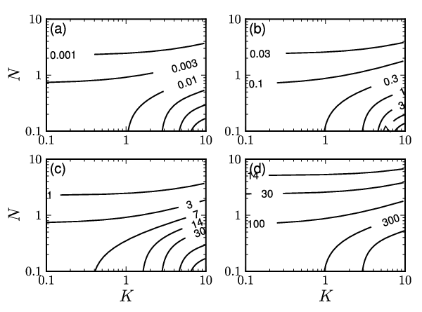
Figure 1 illustrates how depends on stellar parameters. The four panels in Figure 1 display contours of (in days) on the - plane for four different values of . The value of in a neutron star is uncertain but Figure 1 demonstrates that it plays a significant role in determining . One requires for the best match between and observed post-glitch recovery time-scales. This value is artificially lower than that expected from neutron-neutron scattering, (Cutler & Lindblom, 1987; Andersson et al., 2005; van Eysden & Melatos, 2010) because it is the effective value that arises when modelling the two-component Hall-Vinen-Bekarevich-Khalatnikov superfluid (Peralta et al., 2005; Andersson & Comer, 2006) as a single Newtonian fluid (Easson, 1979; Abney & Epstein, 1996; van Eysden & Melatos, 2008).
To calculate , we evaluate (49) with and make several simplifying assumptions. First, we approximate by the leading () terms in the infinite sums in (45)–(48). For typical values of and , this introduces an error of per cent. Second, following Jaranowski et al. (1998), we average the functions and , which oscillate much more rapidly than , , and , over the observation period. The result is
| (50) | |||||
with
| (51) |
As discussed in Section 3.2, the signal is the sum of a persistent periodic signal associated with the fossil nonaxisymmetry (which decays on the long time-scale ) and the decaying signal generated by the Ekman flow. To be conservative, we only consider the latter signal, setting . Hence, (51) reduces to .
The signal-to-noise ratio depends on the right ascension , declination , and polarisation angle of the source as well as the location and orientation of the interferometer and the diurnal phase of the Earth. These quantities are usually known for any specific source. However, to estimate detectability in general, we average over , , , and (Jaranowski et al., 1998):
| (52) |
The beam pattern functions average to
| (53) |
where is the angle between the arms of the detector. We give more details of this result in Appendix B. Substituting (53) into (49) and averaging over , we obtain the following expression for the average signal-to-noise ratio:
| (54) |
4.2 Second- and third-generation interferometers
We now evaluate the signal-to-noise ratio (54) achieved by the second-generation interferometer LIGO, in both its Initial and Advanced configurations, and the third-generation, subterranean Einstein Telescope (ET).

There are various detector configurations proposed for Advanced LIGO11 1 LIGO Document Control Center: document number LIGO-T0900288-v3. The best overall sensitivity across the entire frequency spectrum is achieved with zero detuning of the signal recycling mirror and high laser power. Below 40 Hz, the configuration optimised for 30M⊙ black hole binary inspirals provides the best sensitivity. Above 40 Hz, the configuration optimised for 1.4M⊙ neutron star binary inspirals provides the best sensitivity. However, the differences between the three configurations are small.
Two configurations have been proposed for ET: a conventional interferometer (Hild et al., 2008), and a dual-band ‘xylophone’ configuration consisting of two co-located interferometers, one optimised for low frequencies and the other for high frequencies (Hild et al., 2010). Below 30 Hz, the xylophone configuration is more sensitive than the conventional configuration, by a factor of up to in the 5–-10 Hz band.
Figure 2 compares the spectral noise density of the different detector configurations. It also bins the number of known glitching pulsars and observed glitches as a function of frequency to illustrate which configurations are best suited for glitch searches. It is important to recall that the results of Section 3 predict gravitational radiation at both the pulsar frequency and , with the pulsar orientation determining which frequency has the stronger signal. The xylophone configuration of ET is the best choice for a glitch search. More glitches have been observed in objects with Hz (83 per cent), where the xylophone is more sensitive, than Hz (17 per cent) (Peralta, 2006; Melatos et al., 2008). Additionally, the increase in sensitivity of the ET xylophone configuration over the conventional configuration is far greater below 30 Hz than the decrease above 30 Hz. In contrast, Advanced LIGO is not sensitive below 10 Hz and there is only a small difference in sensitivity between the different configurations over the frequency range where most glitches lie. As mentioned above, the black-hole-optimised Advanced LIGO configuration is the most sensitive below 40 Hz but its advantage is slight and possibly outweighed by its slightly poorer performance at higher frequencies, where the strongest signals (from the fastest-spinning objects) arguably lie.
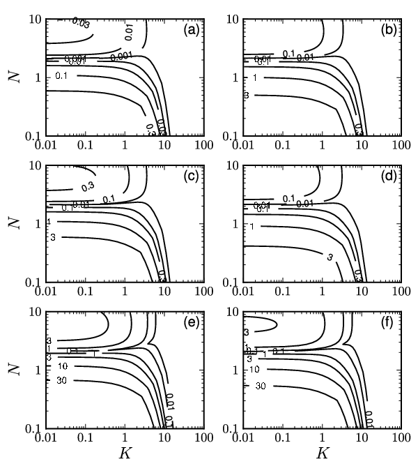
Figure 3 displays contours of the average signal-to-noise ratio for Initial LIGO, Advanced LIGO (zero detuning and high laser power, neutron star optimised, and black hole optimised), and ET (conventional and xylophone) as a function of compressibility and Brunt-Väisälä frequency . The figure is produced for an object with Hz, , at a distance kpc from Earth, with radius km, mass , , and (Ekman pumping occurs in a thin surface layer, where is uniform). The step increase in angular velocity is taken to be , corresponding to the largest glitch observed to date (Melatos et al., 2008). The spectral noise densities used for the six detector configurations are: Initial LIGO , zero-detuning, high-power Advanced LIGO , neutron-star-optimised Advanced LIGO , black-hole-optimised Advanced LIGO , conventional ET , and xylophone ET .
It is clear from Figure 3 that detectability drops off sharply for . Buoyancy prevents Ekman pumping from spinning up the whole of the stellar interior (van Eysden & Melatos, 2008). For large stratification (), , only a small volume of the interior is spun up and the current quadrupole is greatly reduced, with . There is little difference between the three Advanced LIGO configurations in panels (b), (c) and (d), or the two ET configurations displayed in panels (e) and (f) in Figure 3. All have similar sensitivity at 100 Hz. For ET, we find for and and there is a reasonable possibility of detection. We require smaller values, e.g. and , to achieve with Advanced LIGO.
To generalise the results in Figure 3 to an arbitrary object, we note that scales with Ekman number as (square root of the number of cycles in the coherent integration). For relaxation time-scales of 3 to 300 days (Peralta, 2006), and assuming , ranges from to , which corresponds to an order of magnitude of variation in . The signal-to-noise ratio also scales with the spin parameters through the characteristic wave strain, viz.
| (55) |
The relative change in angular velocity is not necessarily equal to the observed glitch size . In a vortex unpinning model, the two quantities are related through , where is the ratio of superfluid to crust moment of inertia, and is the normalised radial distance the unpinned vortices move (Alpar et al., 1986; Melatos & Peralta, 2010). Therefore, equating the observed glitch size to yields a conservative estimate, given that may in fact be up to times larger.
A coherent search synchronised to a radio ephemeris assumes that the radio and gravitational wave signals have the same phase. This is not necessarily true. For example, in the landmark coherent -statistic search for the Crab pulsar in LIGO S5 data, Abbott et al. (2008) allowed for a fractional phase mismatch of up to . In our multiple scales analysis, we assume by construction that the nonaxisymmetric modes are stationary in the frame rotating with the pre-glitch angular velocity and remain so throughout the Ekman pumping process. In reality, the crust spins up to and drags the axisymmetric part of the flow asymptotically to this increased angular velocity. Whether the angular velocity of the modes also increases during this process is unclear. It depends on exactly how the superfluid vortices repin following a glitch and rearrange themselves in a sheared Ekman flow, which is unknown at present.
The number of templates required for a search can be estimated by modelling the frequency as . For a coherent search, the difference in phase between the model and gravitational-wave signals over the integration time must satisfy . For a two week integration, this corresponds to a maximum template spacing of Hz and s-2.
During the glitch recovery, the frequency derivative is much larger than usual for an isolated pulsar spinning down electromagnetically. We approximate . Conservatively, this yields s-2 for a 100 Hz pulsar undergoing the largest glitch observed to date () with an unusually short relaxation period of one day. This translates into a range of s-2 to search over and hence templates in . To allow for some mismatch between the radio and gravitational wave phases we follow Abbott et al. (2008) who searched over a window of Hz centred on the radio frequency, i.e. Hz. Overall, therefore, a total of templates are required for a glitch search.
The parameters , and change the shape of the signal in two ways: the relaxation time is controlled predominantly by , while the relative difference between the signals at and (in amplitude and relaxation time) is controlled by and . Our signal-to-noise ratio estimates in Figure 3 are based on the incoherent sum of the detector response at and , so the relative phasing between and does not affect the detectability and the number of templates required. This would change in a more sophisticated search that combined the and responses coherently.
To this point, we assume that radio observations provide the frequency, recovery time-scale, and trigger epoch for a glitch search. We now consider the scenario where this information is not known, as in a blind search. In the region of parameter space that we consider, , , and , the minimum band width of the Fourier-transformed wave strain is . Hence, searching over the frequency range 1–600 Hz requires templates in multiplied by templates in as discussed above.
In addition, the sky position, time of occurrence, and recovery time are unknown for a blind search. In a LIGO search for unknown periodic sources (Abbott et al., 2007), the sky is divided into 31500 patches. The lack of an electromagnetic trigger means that the data must be searched in many blocks, starting, for example, one day apart (coherent integration over a shorter recovery time is unlikely to be detectable) and integrating over increasing lengths of time, up to the computational limit, to account for the fact that is unknown. A proper estimate of the associated computational expense lies outside the scope of this paper.
5 Constitutive properties of bulk nuclear matter
Figure 3 clearly demonstrates that the strength of the gravitational wave signal depends sensitively on the constitutive properties of bulk nuclear matter (e.g., the equation of state) and its dissipative or transport coefficients (e.g., viscosity). We show that these properties can be inferred in principle from the detailed shape of the gravitational wave signal. The results of this approach can be linked to terrestrial experiments, e.g. with heavy ion colliders, although there is an important distinction between GeV collisions of nucleons in a terrestrial particle accelerator and static nucleons at MeV energies in a neutron star.
In a real search, one seeks to extract parameters like and by fitting a template to the interferometer data in the time domain (Clark et al., 2007; Hayama et al., 2008). However, to illustrate the scientific potential of the fitting exercise, we Fourier transform and and focus on the gross features of the spectrum. We neglect the permanent fossil quadrupole (see Section 3.2) and assume that there is no interference between peaks. The four peak amplitudes and four peak widths (at and ) of and provide enough information to solve for , , , , and by matching to the theoretical predictions in (45)–(48). We take ratios to eliminate (which depends on the unknowns , , , and ) and focus on the remaining parameters.
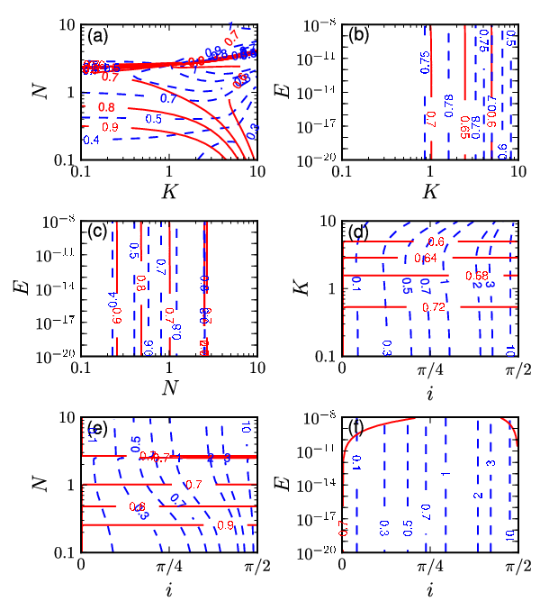
Figure 4 displays six slices through the four-dimensional parameter space. Contours are shown for the amplitude ratio and the width ratio , where is the full width at half maximum of the peak in centred at . The figure is drawn for the parameter ranges , , , and . We evaluate the first 20 terms in the infinite sums in (45)–(48). In those panels where , , , and are held fixed, we use the fiducial values , , , and respectively.
The inclination angle determines the relative strength of the and modes of and through the tensor spherical harmonic in (33). The contours of are nearly vertical in panels (d), (e) and (f) of Figure 4. In fact, if we consider additional amplitude ratios, we can infer independently from the other parameters. Dividing the Fourier transforms of (45) by (47), and (46) by (48), we obtain and respectively. These expressions overdetermine , yielding its value and an independent cross-check. The inclination angle can also be inferred from the radio or gamma-ray pulse profile and polarisation swing by assuming a particular emission model (Lyne & Manchester, 1988; Hibschman & Arons, 2001; Bai & Spitkovsky, 2009; Chung & Melatos, 2010). The width ratios are independent of ; the time-scale over which the signal decays does not depend on the location of the observer. This is illustrated in panels (d), (e) and (f) of Figure 4, where the contours of are horizontal.
The compressibility and Brunt-Väisälä frequency are inextricably linked in the sense that they feed into both the amplitude and width ratios in a complicated manner. However, once we determine according to the formula above, we can immediately extract and from panel (a) of Figure 4 as the value of does not influence any of the amplitude or width ratios (see below). By plotting contours of the measured ratios of and on the - plane, we can read off the values of and from the intersection point of the contours. One might be tempted to use other amplitude and width ratios as a cross-check on and , or to break the degeneracy in the case of multiple intersection points. However, most of the ratios are related trivially through the inclination angle and supply no additional information, e.g. , , and
The Ekman number is important in determining the recovery time-scale and hence the Fourier width. It also appears in through . However, it influences all peaks in the same way and drops out of all amplitude and width ratios. In panels (b), (c) and (f) of Figure 4, the amplitude and width ratio contours are vertical. As mentioned in Section 4, an approximate value of can be inferred from the e-folding time of , as and only weakly influence this quantity. However, if and are known, e.g. by following the procedure described in the above paragraph, we can determine from the absolute peak widths. Finally, can be determined from the absolute peak amplitudes once the values of all the other parameters are known.
Future gravitational-wave measurements of the compressibility, viscosity and Brunt-Väisälä frequency of bulk nuclear matter can be compared to a range of terrestrial experiments and theoretical calculations. The compressibility is commonly expressed in terms of the compression modulus , which is related to our normalised compressibility through , where is the mean atomic number and the proton mass (van Eysden & Melatos, 2008). Heavy-ion collisions and nuclear resonance experiments measure (Sturm et al., 2001; Vretenar et al., 2003; Piekarewicz, 2004; Hartnack et al., 2006). Compressibility can also be inferred from the symmetry energy measured in heavy-ion collisions or obtained through neutron-skin thickness measurements (Chen et al., 2005; Li et al., 2008; Xu et al., 2009). The shear viscosity is often expressed in terms of the ratio , where is the specific entropy. It is related to the Ekman number by where is the entropy per nucleon in units of Boltzmann’s constant (van Eysden & Melatos, 2008). The shear viscosity has also been measured in heavy-ion collisions (Adler et al., 2003; Adare et al., 2007). Neutron stars are stably stratified because the concentration of charged particles increases with density but chemical equilibrium is maintained (Reisenegger & Goldreich, 1992). Stratification provides a buoyancy force proportional to the Brunt-Väisälä frequency squared, which has been calculated theoretically (Reisenegger & Goldreich, 1992; Lai, 1994; Passamonti et al., 2009).
In Table 1 we quote a selection of experimental and theoretical values for , , and under neutron star conditions. Dimensionless values of and assume Hz. In line 1, the compression modulus is inferred from the ratio of the multiplicity in Au+Au and C+C collisions at GeV energies (Sturm et al., 2001; Hartnack et al., 2006). In line 2, the compression modulus is obtained by fitting a relativistic mean-field model to the distribution of isoscalar monopole and isovector dipole strengths of Zr and Pb (Vretenar et al., 2003; Piekarewicz, 2004). In line 3, the compression modulus is obtained from the measured nuclear symmetry energy from isospin diffusion in heavy-ion collisions (Chen et al., 2005; Li et al., 2008). Line 4 lists the ratio of shear viscosity to specific entropy measured in Au+Au collisions at an energy of 200 GeV (Adler et al., 2003; Adare et al., 2007). Theoretical calculations of shear viscosity by Cutler & Lindblom (1987) for neutron-neutron and electron-electron scattering, corresponding to the normal and superfluid states respectively, are listed in lines 5 and 6. More exotic states, which may exist in the neutron star core, will have a different viscosity. Line 7 lists the shear viscosity due to quark-quark scattering (Jaikumar et al., 2008). In lines 8 and 9, we quote calculated values for the Brunt-Väisälä frequency, the latter including centrifugal forces in a rapidly rotating star (Reisenegger & Goldreich, 1992; Lai, 1994; Passamonti et al., 2009).
| Quantity | Experiment/Theory (E/T) | Result | Dimensionless | Reference |
| Au+Au and C+C collisions ( GeV) (E) | MeV | |||
| nuclear resonances (E) | 240–270 MeV | – | ||
| nuclear symmetry energy (E) | MeV | |||
| Au+Au collisions (200 GeV) (E) | ||||
| neutron-neutron scattering (T) | g cm-1 s-1 | |||
| electron-electron scattering (T) | g cm-1 s-1 | |||
| quark-quark scattering (T) | g cm-1 s-1 | |||
| chemical composition (T) | 500 s-1 | |||
| centrifugal correction (T) | - | - | ||
| (1) Sturm et al. (2001), (2) Hartnack et al. (2006), (3) Vretenar et al. (2003), (4) Piekarewicz (2004), (5) Chen et al. (2005), | ||||
| (6) Li et al. (2008), (7) Adler et al. (2003), (8) Adare et al. (2007), (9) Cutler & Lindblom (1987), (10) Jaikumar et al. (2008), | ||||
| (11) Reisenegger & Goldreich (1992), (12) Lai (1994), (13) Passamonti et al. (2009) | ||||
6 Conclusions
In this paper, we calculate analytically the gravitational radiation emitted during the post-glitch recovery phase by the nonaxisymmetric Ekman flow excited by a glitch. The calculation is done in the context of an idealised, cylindrical star with a uniform viscosity, compressibility, and stratification length-scale. We compute the signal-to-noise ratio for current- and next-generation long-baseline interferometers and find the following promising result: for a large glitch () from a neutron star kpc from Earth and spinning at Hz, the angle-averaged signal-to-noise ratio exceeds three for , , and with Advanced LIGO and , , and with ET.
Perhaps the most obvious shortcoming of our idealised model is its cylindrical geometry. There is a noble history of using a cylinder to model spherical astronomical objects and also in classical geophysical studies of the Earth (Pedlosky, 1967; Walin, 1969; Abney & Epstein, 1996; van Eysden & Melatos, 2008), because it admits analytic solutions, which in general have not yet been found for a sphere. We ignore magnetic fields for simplicity, although they are large in neutron stars (Cutler, 2002), interact with the superfluid (Mendell, 1998), and therefore modify Ekman pumping. We model the interior of a neutron star as a single Navier-Stokes fluid, whereas in reality it is a multi-component superfluid, consisting of superfluid neutrons and superconducting protons which interact with each other via mutual friction and entrainment (Lattimer & Prakash, 2004; Andersson & Comer, 2006, e.g.). The spin-up process in a coupled multi-component fluid of this kind, in the presence of gravitational stratification and compressibility, is an unsolved and difficult problem.
In our model, the crust accelerates instantaneously from to and remains at this higher angular velocity. A more realistic model would conserve total angular momentum by solving self-consistently for the response of the crust to the viscous back-reaction torque (van Eysden & Melatos, 2010). In the context of the present model, we can approximate this effect crudely by replacing the glitch size at with the permanent frequency jump after the recovery ceases. None of the conclusions change qualitatively.
Understanding the glitch mechanism remains an unsolved problem. Glitch waiting times are exponentially distributed and their sizes fit a power law (Melatos et al., 2008), indicative of inhomogeneous collective behaviour on large scales, e.g. vortex avalanches. In contrast, nuclear structure calculations suggest that the area density of pinning sites (e.g. lattice defects) is much greater than the area density of vortices (Jones, 2002; Donati & Pizzochero, 2003), suggesting that the system is homogeneous on large scales (pinned Abrikosov array). The gravitational wave signal calculated here helps to discriminate between these two views, as it is a measure of the internal nonaxisymmetry. From a simple, random walk argument, the largest relative glitch size that arises from vortex movement in a star containing vortices is . If the value of inferred from a gravitational-wave detection approaches this maximum, it is safe to infer that large-scale inhomogeneities are present. Note that we take in Section 2.6. However, if only a fraction of the internal flow is nonaxisymmetric, should be reduced in proportion. In vortex unpinning models can be up to four orders of magnitude larger than the observed glitch size (see Section 4.2), leaving considerable scope to get detectable gravitational-wave signals.
Vortex unpinning theories of glitches rely on the build up of a lag between the crust, which spins down electromagnetically, and the superfluid, whose rotation is fixed by the number of vortices, until a glitch is triggered. We know that the lag does not disappear completely after the glitch (i.e. co-rotation is not restored) because a reservoir effect (i.e. glitch size waiting time) is not observed in glitch data (Wong et al., 2001); only a small, random fraction of the lag relaxes during a single event, and that fraction is determined by the microscopic history of the system, as in any avalanche process. In this model, we assume conservatively that the crust and fluid co-rotate before the glitch. However, in the more realistic scenario just described, there is ongoing differential rotation between crust and core, suggesting that glitching pulsars may continuously emit gravitational radiation.
Another possibility leading to a continuous gravitational wave signal beyond just the post-glitch recovery period is the ‘fossil flow’ discussed in Section 3. Stratification prevents Ekman pumping from spinning up the whole interior, leaving a remnant of the initial nonaxisymmetric flow untouched. This flow emits gravitational radiation until damped over the much longer diffusion time-scale. If so, we may be able to extend the coherent integration time beyond the recovery time-scale, increasing the likelihood of detection. Even more intriguing is the possibility that any neutron star which has experienced differential rotation in its past retains some part of this fossil flow for years, thereby bearing an imprint of the star’s formation and rotation history. We plan to study the matter fully in a following paper.
For a typical neutron star at a distance of 1 kpc, the signal-to-noise calculations in Section 4 argue that there is a reasonable chance interferometers like Advanced LIGO or ET will detect the largest glitches. The outlook is more optimistic if we consider nearby ‘dark’ neutron stars. For the estimated galactic population of neutron stars (cf., radio pulsars discovered to date), recent Monte-Carlo simulations predict the closest objects are located pc from Earth (Ofek, 2009). At this distance, Initial LIGO is able to detect the largest glitches with for and and Advanced LIGO is sensitive to smaller glitches with . However, the signal frequency, glitch epoch, and sky position are unknown electromagnetically, so searching for ‘dark’ glitches is a difficult proposition. None the less, our results suggest cautious optimism about the chances of detecting a glitching (or otherwise differentially rotating) neutron star with the next generation of gravitational-wave interferometers.
Acknowledgements
We thank the anonymous referee for their helpful comments and suggestions. MFB and CAVE acknowledge the support of Australian Postgraduate Awards.
References
- Abbott et al. (2007) Abbott B., Abbott R., Adhikari R., Agresti J., Ajith P., Allen B., Amin R., Anderson S. B., Anderson W. G., (…) Lyne A. G., 2007, Physical Review D, 76, 042001
- Abbott et al. (2007) Abbott B., Abbott R., Adhikari R., Agresti J., Ajith P., Allen B., Amin R., Anderson S. B., Anderson W. G., (…) Zweizig J., 2007, Physical Review D, 76, 082001
- Abbott et al. (2008) Abbott B., Abbott R., Adhikari R., Ajith P., Allen B., Allen G., Amin R., Anderson S. B., Anderson W. G., (…) Santostasi G., 2008, The Astrophysical Journal, 683, L45
- Abney & Epstein (1996) Abney M., Epstein R. I., 1996, Journal of Fluid Mechanics, 312, 327
- Adare et al. (2007) Adare A., Afanasiev S., Aidala C., Ajitanand N. N., Akiba Y., Al-Bataineh H., Alexander J., Al-Jamel A., Aoki K., (…) Zolin L., 2007, Physical Review Letters, 98, 172301
- Adler et al. (2003) Adler S. S., Afanasiev S., Aidala C., Ajitanand N. N., Akiba Y., Alexander J., Amirikas R., Aphecetche L., Aronson S. H., (…) Zolin L., 2003, Physical Review Letters, 91, 182301
- Alpar et al. (1986) Alpar M. A., Nandkumar R., Pines D., 1986, The Astrophysical Journal, 311, 197
- Anderson & Itoh (1975) Anderson P. W., Itoh N., 1975, Nature, 256, 25
- Andersson & Comer (2006) Andersson N., Comer G. L., 2006, Classical and Quantum Gravity, 23, 5505
- Andersson et al. (2005) Andersson N., Comer G. L., Glampedakis K., 2005, Nuclear Physics A, 763, 212
- Bai & Spitkovsky (2009) Bai X., Spitkovsky A., 2009, ArXiv e-prints
- Benton & Clark (1974) Benton E. R., Clark A., 1974, Annual Review of Fluid Mechanics, 6, 257
- Bonazzola & Gourgoulhon (1996) Bonazzola S., Gourgoulhon E., 1996, Astronomy and Astrophysics, 312, 675
- Bondarescu et al. (2007) Bondarescu R., Teukolsky S. A., Wasserman I., 2007, Physical Review D, 76, 064019
- Brink et al. (2004) Brink J., Teukolsky S. A., Wasserman I., 2004, Physical Review D, 70, 124017
- Chen et al. (2005) Chen L., Ko C. M., Li B., 2005, Physical Review Letters, 94, 032701
- Chung & Melatos (2010) Chung C. T. Y., Melatos A., 2010, in preparation
- Clark et al. (2007) Clark J., Heng I. S., Pitkin M., Woan G., 2007, Physical Review D, 76, 043003
- Cutler (2002) Cutler C., 2002, Physical Review D, 66, 084025
- Cutler & Lindblom (1987) Cutler C., Lindblom L., 1987, The Astrophysical Journal, 314, 234
- Dodson et al. (2002) Dodson R. G., McCulloch P. M., Lewis D. R., 2002, The Astrophysical Journal, 564, L85
- Donati & Pizzochero (2003) Donati P., Pizzochero P. M., 2003, Physical Review Letters, 90, 211101
- Easson (1979) Easson I., 1979, The Astrophysical Journal, 228, 257
- Greenspan & Howard (1963) Greenspan H. P., Howard L. N., 1963, Journal of Fluid Mechanics, 17, 385
- Hartnack et al. (2006) Hartnack C., Oeschler H., Aichelin J., 2006, Journal of Physics G Nuclear Physics, 32, 231
- Haskell et al. (2006) Haskell B., Jones D. I., Andersson N., 2006, Monthly Notices of the Royal Astronomical Society, 373, 1423
- Hayama et al. (2008) Hayama K., Desai S., Mohanty S. D., Rakhmanov M., Summerscales T., Yoshida S., 2008, Classical and Quantum Gravity, 25, 184016
- Hibschman & Arons (2001) Hibschman J. A., Arons J., 2001, The Astrophysical Journal, 546, 382
- Hild et al. (2008) Hild S., Chelkowski S., Freise A., 2008, ArXiv e-prints
- Hild et al. (2010) Hild S., Chelkowski S., Freise A., Franc J., Morgado N., Flaminio R., DeSalvo R., 2010, Classical and Quantum Gravity, 27, 015003
- Jaikumar et al. (2008) Jaikumar P., Rupak G., Steiner A. W., 2008, Physical Review D, 78, 123007
- Jaranowski et al. (1998) Jaranowski P., Królak A., Schutz B. F., 1998, Physical Review D, 58, 063001
- Jensen (1998) Jensen H. J., 1998, Self-Organized Criticality: Emergent Complex Behavior in Physical and Biological Systems (Cambridge Lecture Notes in Physics). Cambridge University Press
- Jones & Andersson (2002) Jones D. I., Andersson N., 2002, Monthly Notices of the Royal Astronomical Society, 331, 203
- Jones (2002) Jones P. B., 2002, Monthly Notices of the Royal Astronomical Society, 335, 733
- Junk & Egbers (2000) Junk M., Egbers C., 2000, in C. Egbers & G. Pfister ed., Physics of Rotating Fluids Vol. 549 of Lecture Notes in Physics, Berlin Springer Verlag, Isothermal spherical Couette flow. pp 215–+
- Lai (1994) Lai D., 1994, Monthly Notices of the Royal Astronomical Society, 270, 611
- Lattimer & Prakash (2004) Lattimer J. M., Prakash M., 2004, Science, 304, 536
- Lattimer & Prakash (2007) Lattimer J. M., Prakash M., 2007, Physics Reports, 442, 109
- Li et al. (2008) Li B., Chen L., Ko C. M., 2008, Physics Reports, 464, 113
- Lyne & Manchester (1988) Lyne A. G., Manchester R. N., 1988, Monthly Notices of the Royal Astronomical Society, 234, 477
- McCulloch et al. (1990) McCulloch P. M., Hamilton P. A., McConnell D., King E. A., 1990, Nature, 346, 822
- Melatos & Payne (2005) Melatos A., Payne D. J. B., 2005, The Astrophysical Journal, 623, 1044
- Melatos & Peralta (2007) Melatos A., Peralta C., 2007, The Astrophysical Journal, 662, L99
- Melatos & Peralta (2010) Melatos A., Peralta C., 2010, The Astrophysical Journal, 709, 77
- Melatos et al. (2008) Melatos A., Peralta C., Wyithe J. S. B., 2008, The Astrophysical Journal, 672, 1103
- Melatos & Warszawski (2009) Melatos A., Warszawski L., 2009, The Astrophysical Journal, 700, 1524
- Mendell (1998) Mendell G., 1998, Monthly Notices of the Royal Astronomical Society, 296, 903
- Munson & Menguturk (1975) Munson B. R., Menguturk M., 1975, Journal of Fluid Mechanics, 69, 705
- Nakabayashi (1983) Nakabayashi K., 1983, Journal of Fluid Mechanics, 132, 209
- Nayyar & Owen (2006) Nayyar M., Owen B. J., 2006, Physical Review D, 73, 084001
- Ofek (2009) Ofek E. O., 2009, Publications of the Astronomical Society of the Pacific, 121, 814
- Owen et al. (2009) Owen B. J., Reitze D. H., Whitcomb S. E., 2009, in AGB Stars and Related Phenomenastro2010: The Astronomy and Astrophysics Decadal Survey Vol. 2010 of Astronomy, Probing neutron stars with gravitational waves. pp 229–+
- Passamonti et al. (2009) Passamonti A., Haskell B., Andersson N., Jones D. I., Hawke I., 2009, Monthly Notices of the Royal Astronomical Society, 394, 730
- Payne & Melatos (2006) Payne D. J. B., Melatos A., 2006, The Astrophysical Journal, 641, 471
- Pedlosky (1967) Pedlosky J., 1967, Journal of Fluid Mechanics, 28, 463
- Peralta & Melatos (2009) Peralta C., Melatos A., 2009, The Astrophysical Journal, 701, L75
- Peralta et al. (2005) Peralta C., Melatos A., Giacobello M., Ooi A., 2005, The Astrophysical Journal, 635, 1224
- Peralta et al. (2006a) Peralta C., Melatos A., Giacobello M., Ooi A., 2006a, The Astrophysical Journal, 644, L53
- Peralta et al. (2006b) Peralta C., Melatos A., Giacobello M., Ooi A., 2006b, The Astrophysical Journal, 651, 1079
- Peralta et al. (2008) Peralta C., Melatos A., Giacobello M., Ooi A., 2008, Journal of Fluid Mechanics, 609, 221
- Peralta (2006) Peralta C. A., 2006, PhD thesis, University of Melbourne, Australia
- Piekarewicz (2004) Piekarewicz J., 2004, Physical Review C, 69, 041301
- Reisenegger & Goldreich (1992) Reisenegger A., Goldreich P., 1992, The Astrophysical Journal, 395, 240
- Sedrakian et al. (2003) Sedrakian D. M., Benacquista M., Shahabassian K. M., Sadoyan A. A., Hairapetyan M. V., 2003, Astrophysics, 46, 445
- Shemar & Lyne (1996) Shemar S. L., Lyne A. G., 1996, Monthly Notices of the Royal Astronomical Society, 282, 677
- Sidery et al. (2009) Sidery T., Passamonti A., Andersson N., 2009, ArXiv e-prints
- Sturm et al. (2001) Sturm C., Böttcher I., Dȩbowski M., Förster A., Grosse E., Koczoń P., Kohlmeyer B., Laue F., Mang M., (…) Waluś W., 2001, Physical Review Letters, 86, 39
- Thorne (1980) Thorne K. S., 1980, Reviews of Modern Physics, 52, 299
- Ushomirsky et al. (2000) Ushomirsky G., Cutler C., Bildsten L., 2000, Monthly Notices of the Royal Astronomical Society, 319, 902
- van Eysden & Melatos (2008) van Eysden C. A., Melatos A., 2008, Classical and Quantum Gravity, 25, 225020
- van Eysden & Melatos (2010) van Eysden C. A., Melatos A., 2010, Monthly Notices of the Royal Astronomical Society (submitted)
- Vigelius & Melatos (2009) Vigelius M., Melatos A., 2009, Monthly Notices of the Royal Astronomical Society, 395, 1972
- Vretenar et al. (2003) Vretenar D., Nikšić T., Ring P., 2003, Physical Review C, 68, 024310
- Walin (1969) Walin G., 1969, Journal of Fluid Mechanics, 36, 289
- Warszawski & Melatos (2008) Warszawski L., Melatos A., 2008, Monthly Notices of the Royal Astronomical Society, 390, 175
- Wong et al. (2001) Wong T., Backer D. C., Lyne A. G., 2001, The Astrophysical Journal, 548, 447
- Xu et al. (2009) Xu J., Chen L., Li B., Ma H., 2009, Physical Review C, 79, 035802
Appendix A Simplifying
It is straightforward to evaluate by substituting (23)–(27) directly into (34). However, the calculation is easier and more transparent if we first simplify the integrand in (34) to depend only on . Expanding according to , , we express the integrand to first order as
| (56) |
The first term in (56) is independent of time. It does not emit gravitational radiation, so we discard it. The second term in (56) reads
| (57) | |||||
| (58) |
To move from (57) to (58) we use the Navier-Stokes equation (1) to first order in Rossby number and zeroth order in Ekman number. In the rotating frame and neglecting the centrifugal term, as in Section 2, it reads
| (59) |
from which we obtain
| (60) |
The third term in (56) can be rewritten in a similar way. From (59), we find
| (61) |
where are the basis vectors in cylindrical coordinates. Noting that , as the axial flow is , we are left with
| (62) |
and the third term in (56) is
| (63) |
Combining (58) and (63), and replacing by , we arrive at
| (64) |
There is a subtle issue around neglecting the centrifugal correction to (59), which is of order . If we evaluate by substituting (23)–(27) directly into (34), we implicitly include centrifugal terms in (by virtue of failing to exclude them explicitly). This approach is internally inconsistent, because centrifugal terms of this order are excluded from the flow fields (23)–(27) following the assumption in Section 2.2 leading to (5) and (6). It is therefore preferable to evaluate (34) for using (64), so that the centrifugal correction to the zeroth-order structure is consistently excluded from both the flow fields and .
Appendix B Beam pattern functions
The complete expressions for the beam pattern functions are (Jaranowski et al., 1998),
| (65) | |||||
| (66) |
with
| (67) | |||||
| (68) | |||||
The right ascension and declination of the gravitational wave source are given by and respectively, and is the polarisation angle. The latitude of the detector is denoted by , is the angular velocity of the Earth, and is the diurnal phase of the Earth. The angle counterclockwise between East and the bisector of the interferometer arms is , and the angle between the arms of the interferometer is . We average over , and according to (Jaranowski et al., 1998)
| (69) |
We evaluate and for use in Section 4. Averaging (65) and (66) over , we obtain
| (70) |
All the dependence on and is contained in and . After some straightforward but lengthy algebra, we find that the dependence on all other angles drops out, leaving
| (71) |
Substituting (71) into (70) and evaluating the now trivial time integration we obtain the result stated in equation (53),
| (72) |