Fast Mixing of Parallel Glauber Dynamics and Low-Delay CSMA SchedulingThanks: Authors names appear in the alphabetical order of their last names.Thanks: This work is supported by MURI grant BAA 07-036.18, NSF Grants 07-21286, 05-19691, 03-25673, AFOSR Grant FA-9550-08-1-0432 and DTRA Grant HDTRA1-08-1-0016.

Libin Jiang Affiliation: UC Berkeley
ljiang@eecs.berkeley.edu Mathieu Leconte Affiliation: Technicolor Paris Lab
mathieu.leconte@technicolor.com Jian Ni Affiliation: UIUC
jianni@illinois.edu R. Srikant Affiliation: UIUC
rsrikant@illinois.edu Jean Walrand Affiliation: UC Berkeley
wlr@eecs.berkeley.edu

Abstract

Glauber dynamics is a powerful tool to generate randomized, approximate solutions to combinatorially difficult problems. It has been used to analyze and design distributed CSMA (Carrier Sense Multiple Access) scheduling algorithms for multi-hop wireless networks. In this paper we derive bounds on the mixing time of a generalization of Glauber dynamics where multiple links are allowed to update their states in parallel and the fugacity of each link can be different. The results can be used to prove that the average queue length (and hence, the delay) under the parallel Glauber dynamics based CSMA grows polynomially in the number of links for wireless networks with bounded-degree interference graphs when the arrival rate lies in a fraction of the capacity region. We also show that in specific network topologies, the low-delay capacity region can be further improved.

I Introduction

In wireless networks, the links (transmitter-receiver pairs) may not be able to transmit simultaneously due to interference. A scheduling algorithm, or MAC (Medium Access Control) protocol, determines which links can access the medium in each time instant so that no active links interfere with each other. Since many wireless network applications today have stringent bandwidth and delay requirements but the resources (e.g., spectrum, power) are often quite limited in a wireless setting, designing low-complexity scheduling algorithms to achieve high throughput and low delay is of great importance.

It is well known that the queue-length based Maximum Weighted Scheduling (MWS) algorithm is throughput-optimal [21], meaning that it can stabilize the network queues for all arrival rates in the capacity region of the network. However, MWS requires the network to select a max-weight independent set in the interference graph in every time slot, which is NP-hard for general interference graphs [5]. There exist several low-complexity alternatives such as Maximal Scheduling and Greedy Maximal Scheduling, but in general these algorithms can only guarantee to achieve a fraction of the capacity region (see [12] and references therein).

Due to their simplicity, random access type scheduling algorithms such as Aloha and Carrier Sense Multiple Access (CSMA) are widely used in practice. Performance analysis of random access algorithms in single-hop wireless networks can be found in [1]. In [2] the authors introduced a continuous-time Markov chain model to analyze the performance of a (fixed-parameter) CSMA algorithm in multi-hop wireless networks, and it was shown that the stationary distribution over the schedules has a product form. The model was used in [23] to study throughput and fairness issues of the CSMA algorithm, and its insensitivity properties were studied in [13]. A discrete-time version of the algorithm was studied in [16, 17].

In [10] the authors proposed an adaptive CSMA algorithm where the links adaptively adjust their parameters based on locally measured arrival and service rates. The algorithm was shown to be throughput-optimal under a time-scale separation assumption (the CSMA Markov chain converges to its steady-state distribution instantaneously compared to the time-scale of adaptation of the CSMA parameters) which can be justified using a stochastic-approximation argument [14, 11]. In [18] the authors established throughput-optimality of their adaptive CSMA algorithm without the time-scale separation assumption by choosing the link parameters to be slowly varying functions of the queue lengths. The discrete-time equivalent of this analysis for the model in [16, 17] appears in [6].

Central to these CSMA algorithms is the so-called Glauber dynamics, which is a Markov Chain Monte Carlo method that can be used to sample the independent sets of a graph according to a product-form distribution [4, 22]. Under traditional Glauber dynamics, in each time slot one link will be selected uniformly at random, and only that link can change its state while other links will keep their states unchanged. For the chosen link, if all of its neighboring links were in state $0$ (inactive) in the previous slot, then the link will choose to be in state $1$ (active) with probability $\frac{\lambda}{1+\lambda}$ and in state $0$ with probability $\frac{1}{1+\lambda}$ ; otherwise (i.e., if at least one of its neighboring links was in state $1$ in the previous slot), the link will choose to be in state $0$ definitely. In statistical physics, the parameter $\lambda$ is called the fugacity since it indicates how likely a selected site will change its state.¹¹ 1 And the same fugacity $\lambda$ is shared by all links under the traditional Glauber dynamics. In the current paper, however, we need to consider heterogeneous fugacities. That is, different links have different fugacities. Glauber dynamics has many applications in statistical physics, graph coloring, approximate counting, and combinatorial optimization (e.g., [4, 15, 22]). In these applications, the performance of the Glauber dynamics is often determined by how fast the Markov chain converges to the stationary distribution. The Glauber dynamics is said to be fast mixing if the mixing time (will be defined formally later) grows polynomially in the size of the graph. The algorithm in [16, 17] is a generalization of Glauber dynamics where multiple links are allowed to update their states in parallel. The CSMA algorithm in [2] can be viewed as continuous-time Glauber dynamics with fixed parameters, and the CSMA algorithms in [10, 18] can be viewed as continuous-time Glauber dynamics with adaptive parameters. In this paper, we focus on the discrete-time CSMA algorithm suggested in [16, 17]. An important feature of this algorithm is that the overhead for signaling is constant (independent of the size of the network) even taking into account the collisions during the signaling phase. The results in this paper can be extended to other versions of CSMA algorithms as well.

The recently proposed Glauber dynamics based CSMA algorithms have made an important progress to the design of low-complexity distributed scheduling algorithms to achieve maximum throughput in wireless networks. On the other hand, the delay performance of these CSMA algorithms has not been well understood. As shown in a recent work [20], for general networks, it may not be possible to design low-complexity scheduling algorithms which can achieve both low delay (i.e., grows polynomially in the number of links) and even a diminishingly small fraction (i.e., approaches zero when the number of links increases) of the capacity region unless $\mathbf{NP}\subseteq\mathbf{BPP}$ or $\mathbf{P}=\mathbf{NP}$ . In this paper we prove a positive result. We show that our parallel Glauber dynamics based CSMA scheduling algorithm can achieve both low delay and a fraction (independent of the size of the network) of the capacity region when the interference graphs satisfy certain properties.

The main contributions of this paper include:

•

We analyze the mixing time of Glauber dynamics with parallel updates and heterogenous fugacities. We derive various conditions on the system parameters such as fugacities, vertex degrees and update probabilities, under which the mixing time grows logarithmically in the number of vertices.
•

Based on the above mixing time results, we show that, for wireless networks with bounded-degree interference graphs, the parallel Glauber dynamics based CSMA algorithm can achieve a small queue length ( $O(\log n)$ where $n$ is the number of links in the network) at each link if the arrival rate lies within a fraction (independent of $n$ ) of the capacity region and the fugacities of the links are appropriately chosen and fixed. Moreover, we consider an adaptive version of the CSMA algorithm where the fugacities of the links are adjusted based on local queue length information. We show that the total queue length in the network grows polynomially ( $O(n^{3}\log n)$ ) under the adaptive CSMA algorithm.
•

Unlike prior analysis of Glauber dynamics based CSMA algorithms which uses the conductance method to obtain exponential bounds on the mixing time and the queue lengths, here we use the coupling method which allows us to obtain polynomial bounds on the queue lengths for a fraction of the capacity region.
•

For a special but important network topology (Wireless LANs), we show that Glauber dynamics based CSMA can support the full capacity region with linear mixing time.

In a related work [19], the authors proposed a CSMA algorithm which can achieve order-optimal delay performance (i.e., the per-node delay is bounded by a constant) for networks with polynomial growth structure (the number of $r$ -hop neighbors of any node is bounded by a polynomial of $r$ ). The key idea is to (periodically) partition the network into sub-networks with bounded number of nodes in each sub-network such that the mixing time of the Markov chain of the schedule in each sub-network is bounded by a constant. However, the partition is realized by a distributed coloring algorithm which requires the nodes to exchange messages with their multi-hop neighbors, and this overhead can be significant and may increase with the size of the network, especially when the discrete nature of signaling is considered. So a direct comparison of our results and the results in [19] appears to be difficult.

The paper is organized as follows. In Section II we introduce a CSMA scheduling algorithm based on a generalization of Glauber dynamics with parallel updates and heterogenous fugacities. In Section III we derive bounds on the mixing time of parallel Glauber dynamics, with the proof presented in Section IV. In Section V we analyze the delay performance of the CSMA scheduling algorithms using the mixing time results. Section VI is dedicated to the analysis of complete interference graphs. The paper is concluded in Section VII.

II CSMA Scheduling Based on Parallel Glauber dynamics

For a wireless link $i$ , we use $\mathcal{N}_{i}$ to denote the set of conflicting links (called conflict set or neighbor set) of link $i$ : if any link in $\mathcal{N}_{i}$ is active (transmitting), then link $i$ cannot be active.

The interference relationship among the wireless links can be represented by the so-called interference graph (or conflict graph) $G=(V,E)$ , where the vertices in $V$ represent wireless links in the network, and there is an edge between two vertices in $G$ if the corresponding wireless links interfere with each other. (For example, Fig.1(a) shows a wireless network of 3 links, where link $2$ interferes with links $1$ and $3$ , and links $1$ and $3$ don’t interfere with each other. So, the associated interference graph is shown in Fig.1(b), and the conflict set of link 2 is $\mathcal{N}_{2}=\{1,3\}$ , etc.) An independent set of $G$ is a subset of the vertices in $V$ where no two vertices are neighbors of each other. Let $\mathcal{I}$ be the set of all independent sets of $G$ .

Refer to caption — Fig. 1: An example network and the corresponding interference graph.

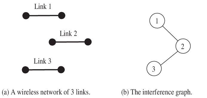
A feasible schedule of the network is a set of wireless links that can be active at the same time according to the conflict set constraint, i.e., no two links in a feasible schedule conflict with each other. This corresponds to an independent set of vertices in the interference graph. (In Fig.1(b), for example, the sets $\{1\},\{1,3\},\{2\}$ are all feasible schedules.) We will use links and vertices interchangeably throughout this paper.

Suppose $|V|=n$ . We can represent a feasible schedule by a vector $\sigma$ of the form $(\sigma_{i})_{i\in V}$ , with $\sigma_{i}\in\mathcal{X}=\{0,1\}$ for all $i\in V$ . For a link $i$ and a schedule $\sigma$ , we say link $i$ is included in the schedule (written as $i\in\sigma$ ) if $\sigma_{i}=1$ . Note that $\sigma$ is a feasible schedule if the set $\{i\in V:\sigma_{i}=1\}$ is an independent set of $G$ , i.e., if $\sigma_{i}+\sigma_{j}\leq 1,\mbox{ for all }(i,j)\in E.$ Let $\Omega\subseteq\mathcal{X}^{n}$ be the set of all feasible schedules on $G$ .

We consider a time-slotted system. A scheduling algorithm is a procedure to decide which schedule to be used in every time slot for data transmission. In [16] we proposed a scheduling algorithm based on a generalization of Glauber dynamics (called parallel Glauber dynamics) where multiple links are allowed to update their states in a single time slot. The key idea is that in every time slot, we select an independent set of links $\mathbf{m}\in\mathcal{I}$ to update their states according to a randomized procedure, i.e., we select $\mathbf{m}\in\mathcal{I}$ with probability $q_{\mathbf{m}}$ , where $\sum_{\mathbf{m}\in\mathcal{I}}q_{\mathbf{m}}=1.$ We call $\mathbf{m}$ the decision schedule.²² 2 A distributed mechanism to generate the decision schedule, as suggested in [16], is the following. At the beginning of a slot, each link independently transmits a short INTENT message with probability $a\in(0,1)$ . A link is included in the decision schedule if (and only if) it sends an INTENT message while none of its neighbors sends such a message.

The parallel Glauber dynamics is formally described as follows.

Parallel Glauber Dynamics (in Time Slot $t$ )

1.

Randomly choose a decision schedule $\mathbf{m}(t)\in\mathcal{I}$ with probability $q_{\mathbf{m}(t)}$ .
2.

For every link $i\in\mathbf{m}(t)$ :
aa If $\sum_{j\in\mathcal{N}_{i}}\sigma_{j}(t-1)=0$
aaaa (a) $\sigma_{i}(t)=1$ with probability $p_{i}=\frac{\lambda_{i}}{1+\lambda_{i}}.$
aaaa (b) $\sigma_{i}(t)=0$ with probability $\bar{p}_{i}=\frac{1}{1+\lambda_{i}}.$
aa Else
aaaa (c) $\sigma_{i}(t)=0$ .
For every link $j\notin\mathbf{m}(t):$
aaaa (d) $\sigma_{j}(t)=\sigma_{j}(t-1)$ .

Under the Parallel Glauber Dynamics based CSMA (called PGD-CSMA for short), $\sigma(t)$ is used as the transmission schedule in time slot $t$ : link $i$ will transmit a data packet if $\sigma_{i}(t)=1$ , and will keep silent if $\sigma_{i}(t)=0$ . Note that link $i$ knows whether $\sum_{j\in\mathcal{N}_{i}}\sigma_{j}(t-1)=0$ by conducting carrier sensing in time slot $t-1$ : the channel (medium) will be sensed idle if none of its neighboring links were transmitting (i.e., $\sum_{j\in\mathcal{N}_{i}}\sigma_{j}(t-1)=0$ ). $p_{i}$ is called the link activation probability, which is determined by the fugacity $\lambda_{i}$ of link $i$ .

We can show that if the transmission schedule used in the previous slot and the decision schedule used in the current slot both are feasible, then the transmission schedule generated in the current slot is also feasible [16]. Moreover, given the fugacities $\lambda_{i}$ ’s, because $\sigma(t)$ only depends on the previous schedule $\sigma(t-1)$ and some randomly selected decision schedule $\mathbf{m}(t)$ , $\sigma(t)$ evolves as a discrete-time Markov chain (DTMC).

Theorem 1

([16]) A necessary and sufficient condition for the parallel Glauber dynamics to be irreducible and aperiodic is $\cup_{\mathbf{m}\in\mathcal{I}:q_{\mathbf{m}}>0}\mathbf{m}=V,$ or equivalently, the probability of selecting link $i$ in the decision schedule $q_{i}:=\sum_{\mathbf{m}\ni i}q_{\mathbf{m}}>0$ for all $i\in V$ . In this case the Markov chain is reversible and has the following product-form stationary distribution:

\displaystyle\pi(\sigma)

\displaystyle=

\displaystyle\frac{\prod_{i\in\sigma}\lambda_{i}}{\sum_{\sigma^{\prime}\in\Omega}\prod_{i\in\sigma^{\prime}}\lambda_{i}}.

(1)

Based on the product-form distribution, one can establish throughput-optimality of PGD-CSMA by either choosing the link activation probabilities (fugacities) as appropriate increasing functions of the (time-varying) queue lengths, or adjusting the fugacities based on the measured arrival and service rates, as in [10, 16, 18]. The focus of this paper is to analyze the mixing time of parallel Glauber dynamics and the delay performance of PGD-CSMA. We will show that the parallel Glauber dynamics is fast mixing when the fugacities satisfy certain conditions, and this implies that PGD-CSMA induces small queue lengths when the arrival rates lie in a fraction of the capacity region.

III Mixing Time of Parallel Glauber Dynamics

III-A Definitions

Consider a finite-state, irreducible, aperiodic Markov chain $(P,\Omega,\pi)$ where $P$ denotes the transition matrix, $\Omega$ denotes the state space, and $\pi$ denotes the unique stationary distribution. First we describe a notion of distance between distributions.

Definition 1

The variation distance between two distributions $\mu,\mu^{\prime}$ on $\Omega$ is defined as

\displaystyle||\mu-\mu^{\prime}||_{var}=\frac{1}{2}\sum_{x\in\Omega}|\mu(x)-\mu^{\prime}(x)|.

(2)

Note that $0\leq||\mu-\mu^{\prime}||_{var}\leq 1$ and $||\mu-\mu^{\prime}||_{var}=0$ if and only if $\mu=\mu^{\prime}$ .

Definition 2

The mixing time $T_{mix}$ of the Markov chain is defined as the time required for the Markov chain to get close to the stationary distribution. More precisely,

\displaystyle T_{mix}=\max_{x\in\Omega}\inf\Big\{t:||\mu_{x,t}-\pi||_{var}\leq\frac{1}{e}\Big\}

(3)

where $\mu_{x,t}$ is the distribution of the Markov chain at time $t$ if the Markov chain starts with state $x$ .

III-B Conditions for fast mixing of Parallel Glauber Dynamics

We now state the main theorem of this section and a corollary on the mixing time of parallel Glauber dynamics with fixed fugacities $\bm{\lambda}$ . The proof of the main theorem will be presented in the next section.

We associate a weight $f(v)>0$ to each vertex (or link) $v\in V$ , and call $f(\cdot)$ the weight function.

Theorem 2

For any positive weight function $f(v)$ of $v\in V$ , let $m=\min_{v\in V}f(v)$ , $M=\max_{v\in V}f(v)$ , and $\xi=\frac{M}{m}$ . If

\displaystyle\theta\triangleq\min_{v\in V}\left\{q_{v}f(v)-\sum_{w\in\mathcal{N}_{v}}q_{w}\frac{\lambda_{w}}{1+\lambda_{w}}f(w)\right\}>0,

(4)

where $q_{v}$ , as defined before, is the probability that vertex $v$ is included in the decision schedule, then under the parallel Glauber dynamics,

||\mu_{x,t}-\pi||_{var}\leq\min\Big\{1,(1-\frac{\theta}{M})^{t}n\xi\Big\},\forall x\in\Omega.

(5)

Therefore the parallel Glauber dynamics is fast mixing and its mixing time is bounded by:

\displaystyle T_{\textit{mix}}

\displaystyle\leq

\displaystyle\bar{T}_{mix}=\Big\lceil\frac{M}{\theta}\log(n\xi e)\Big\rceil.

(6)

One can specify the weight function $f(\cdot)$ to obtain various conditions on the fugacities for fast mixing. We will show one of them below which will be used later to analyze the delay performance of PGD-CSMA. Other conditions are given in Appendix -A.

Corollary 1

Let $m=\min_{v\in V}\frac{d_{v}}{q_{v}}$ , $M=\max_{v\in V}\frac{d_{v}}{q_{v}}$ and $\xi=\frac{M}{m}$ , where $d_{v}$ is the degree of $v$ in the interference graph. If $\lambda_{v}<\frac{1}{d_{v}-1}$ for all $v\in V$ , then

\displaystyle T_{\textit{mix}}

\displaystyle\leq

\displaystyle\bar{T}_{\textit{mix}}=\Big\lceil\frac{M}{\theta}\log(n\xi e)\Big\rceil,

(7)

where

\displaystyle\theta=\min_{v\in V}\left\{d_{v}-\sum_{w\in\mathcal{N}_{v}}\frac{\lambda_{w}}{1+\lambda_{w}}d_{w}\right\}.

(8)

Proof:

Choose $f(v)=\frac{d_{v}}{q_{v}}$ . By Theorem 2, the parallel Glauber dynamics is fast mixing if θ=min_v∈V{d_v-∑_w∈N_v λ w 1+λ w d_w}¿0.

To achieve that, we need $\forall v\in V$ , $d_{v}-\sum_{w\in\mathcal{N}_{v}}\frac{\lambda_{w}}{1+\lambda_{w}}d_{w}>0.$ It is sufficient to have $\frac{\lambda_{w}}{1+\lambda_{w}}d_{w}<1$ , $\forall w\in V$ , which is equivalent to $\lambda_{w}<\frac{1}{d_{w}-1}$ . ∎

Remark 1

Let $\Delta$ be the maximum vertex degree of $G$ . If each link (vertex) sends the INTENT message independently with probability 1/2, then $(1/2)^{\Delta+1}\leq q_{v}\leq 1$ , so $m\geq 1$ and $M\leq\Delta\cdot 2^{\Delta+1}$ . Then we have

\bar{T}_{\textit{mix}}\leq\Big\lceil\frac{\Delta\cdot 2^{\Delta+1}}{\theta}\log(\Delta\cdot 2^{\Delta+1}en)\Big\rceil,

i.e., the mixing time grows as $O(\log n)$ for bounded-degree graphs when $\lambda_{v}<\frac{1}{\Delta-1}\leq\frac{1}{d_{v}-1},\forall v$ . On the other hand, it was shown in [8] that traditional single-site Glauber dynamics has a mixing time at least $\Omega(n\log n)$ for bounded-degree graphs. Therefore, parallel Glauber dynamics reduces the mixing time by an order of magnitude.

Remark 2

For interference graphs with special structure, more relaxed conditions can be obtained to ensure fast mixing. This will be discussed in Section VI.

IV Proof of Fast Mixing

This section presents the proof of Theorem 2. In particular, we use the coupling method to establish the logarithmic mixing time. Readers who are only interested in the main results could skip the section without loss of continuity.

IV-A Preliminaries

A useful technique to bound the mixing time of a Markov chain is via coupling.

Definition 3

A coupling of the Markov chain is a stochastic process $(X(t),Y(t))$ on $\Omega\times\Omega$ such that $\{X(t)\}$ and $\{Y(t)\}$ marginally are copies the original Markov chain, and if $X(t)=Y(t)$ , then $X(t+1)=Y(t+1)$ .

Let $\Phi$ be a distance function (metric) defined on $\Omega\times\Omega$ , which satisfies that for any $x,y,z\in\Omega$ : (1) $\Phi(x,y)\geq 0$ , with equality if and only if $x=y$ ; (2) $\Phi(x,y)=\Phi(y,x)$ ; (3) $\Phi(x,z)\leq\Phi(x,y)+\Phi(y,z).$ Let

D_{min}=\min_{x\neq y}\Phi(x,y),D_{max}=\max_{x,y}\Phi(x,y),D=\frac{D_{max}}{D_{min}}.

The following theorem (e.g., [4]) can be used to bound the mixing time of the Markov chain.

Theorem 3

Suppose $(X(t),Y(t))$ is coupling of the Markov chain where $X(t)$ has distribution $\mu_{t}$ and $Y(t)$ has distribution $\mu^{\prime}_{t}=\pi$ . If there exists some constant $\beta<1$ such that, for all $x,y\in\Omega$ ,

E[\Phi(X(t+1),Y(t+1))|X(t)=x,Y(t)=y]\leq\beta\Phi(x,y).

(9)

Then

\displaystyle||\mu_{t}-\pi||_{var}

\displaystyle\leq

\displaystyle\min\{1,\beta^{t}D\}

(10)

and the mixing time of the Markov chain is bounded by:

\displaystyle T_{mix}\leq\Big\lceil\frac{\log(De)}{\log\beta^{-1}}\Big\rceil\leq\Big\lceil\frac{\log(De)}{1-\beta}\Big\rceil\doteq\bar{T}_{mix}.

(11)

In general, determining $\beta$ in the contraction condition (9) is hard since we need to check the condition for all pairs of configurations $(x,y)$ . In [3] the so-called path coupling method was introduced by Bubley and Dyer to simplify the calculation. Using path coupling, we only need to check the contraction condition for certain pairs of configurations. The path coupling method is described in the following theorem.

Theorem 4

Let $S\subseteq\Omega\times\Omega$ and suppose that for all $x,y\in\Omega\times\Omega$ , there exists a path $x=z_{0},z_{1},\ldots,z_{r}=y$ between $x$ and $y$ such that $(z_{l},z_{l+1})\in S$ for $0\leq l<r$ and $\Phi(x,y)=\sum_{l=0}^{r-1}\Phi(z_{l},z_{l+1}).$ Suppose $(X(t),Y(t))$ is a coupling of the Markov chain as in Theorem 3. If there exists $\beta<1$ such that for any $(x,y)\in S$ , the contraction condition (9) holds, then we have (10) and the mixing time of the Markov chain is bounded as in (11).

Note that the key simplification in the path coupling theorem (Theorem 4), compared to the coupling theorem (Theorem 3), is that the contraction condition (9) needs to hold only for $(x,y)\in S$ , instead of $(x,y)\in\Omega\times\Omega$ .

IV-B Proof of Fast Mixing

Now we analyze the mixing time of Glauber dynamics with parallel updates and heterogenous fugacities using the path coupling technique. We use the following distance function between feasible schedules. For any $\sigma,\eta\in\Omega$ , let

\displaystyle\Phi(\sigma,\eta)=\sum_{v}|\sigma_{v}-\eta_{v}|f(v)=\sum_{v\in\sigma\bigtriangleup\eta}f(v),

(12)

where $f(v)>0$ is the weight function of $v\in V$ and $\sigma\bigtriangleup\eta=(\sigma\setminus\eta)\cup(\eta\setminus\sigma)$ is the symmetric difference between $\sigma$ and $\eta$ . Note that the distance function is a weighted Hamming distance function and satisfies all the properties of a metric.

Consider the following coupling $(\sigma(t),\eta(t))$ : in every time slot both chains select the same decision schedule and use the same coin toss for every vertex in the decision schedule if that vertex can be added to both schedules.

Let $E[\Delta\Phi(\sigma,\eta)]$ be the (conditional) expected change of the the distance between the states of the two Markov chains $\{\sigma(t)\}$ and $\{\eta(t)\}$ after one slot:

	$\displaystyle E[\Delta\Phi(\sigma,\eta)]$	$\displaystyle=$	$\displaystyle E[\Phi(\sigma(t+1),\eta(t+1)\|\sigma(t)=\sigma,\eta(t)=\eta]$
			$\displaystyle-\Phi(\sigma,\eta).$

For any $\mathbf{m}\in\mathcal{I}$ , let

E[\Delta^{\mathbf{m}}\Phi(\sigma,\eta)]=E[\Delta\Phi(\sigma,\eta)|\mathbf{m}\mbox{ is the decision schedule}].

We say that $\sigma,\eta\in\Omega$ are adjacent and we write $\sigma\sim\eta$ if there exists $v\in V$ such that $\sigma$ and $\eta$ differ only at $v$ . Let

S=\{(\sigma,\eta):\sigma,\eta\in\Omega\mbox{ and }\sigma\sim\eta\}

be the set of all pairs of adjacent schedules. Note that under the distance function defined in (12), for all $\sigma,\eta\in\Omega$ , we can find a path $\sigma=\tau_{0},\tau_{1},\ldots,\tau_{|\sigma\triangle\eta|}=\eta$ between $\sigma$ and $\eta$ such that $(\tau_{l},\tau_{l+1})\in S$ for $0\leq l<|\sigma\triangle\eta|$ and

\Phi(\sigma,\eta)=\sum_{l=0}^{|\sigma\triangle\eta|-1}\Phi(\tau_{l},\tau_{l+1}).

Lemma 1

Consider a pair of adjacent schedules $\sigma$ and $\eta$ that differ only at $v$ (so $\Phi(\sigma,\eta)=f(v)$ ),

\displaystyle E[\Delta\Phi(\sigma,\eta)]\leq-q_{v}f(v)+\sum_{w\in\mathcal{N}_{v}}q_{w}\frac{\lambda_{w}}{1+\lambda_{w}}f(w).

(13)

Proof:

Without loss of generality, suppose $\sigma_{v}=0$ and $\eta_{v}=1.$ Note that $\eta_{v}=1$ implies that $\eta_{w}=0$ for all $w\in\mathcal{N}_{v}$ . Since, $\sigma$ and $\eta$ differ only at $v$ , this also means that $\sigma_{w}=0$ for all $w\in\mathcal{N}_{v}$ . We have

			$\displaystyle E[\Delta\Phi(\sigma,\eta)]$
		$\displaystyle=$	$\displaystyle E_{\mathbf{m}}\Big[E[\Delta^{\mathbf{m}}\Phi(\sigma,\eta)]\Big]=\sum_{\mathbf{m}\in\mathcal{I}}q_{\mathbf{m}}E[\Delta^{\mathbf{m}}\Phi(\sigma,\eta)]$
		$\displaystyle=$	$\displaystyle\sum_{\mathbf{m}\in\mathcal{I}}q_{\mathbf{m}}\sum_{y\in\mathbf{m}}E[\Delta^{y}\Phi(\sigma,\eta)]=\sum_{y\in V}q_{y}E[\Delta^{y}\Phi(\sigma,\eta)].$

Note that only updates on vertices $v$ and $w\in\mathcal{N}_{v}$ can affect the value of $E[\Delta\Phi(\sigma,\eta)]$ because updates on other vertices will have the same outcomes due to coupling.

If $v$ is selected for update and since we use the same coin toss for both Markov chains, then $\sigma(t+1)=\eta(t+1)$ and $\Phi(\sigma(t+1),\eta(t+1))=0$ . Thus $E[\Delta^{v}\Phi(\sigma,\eta)]=-f(v)$ .

If $w\in\mathcal{N}_{v}$ is selected for update, under schedule $\eta,$ $w$ can only take value $0$ because $w$ has a neighbor (i.e., $v$ ) belongs to $\eta$ . While under schedule $\sigma,$ there are two cases:
(1) if $w$ has a neighbor in $\sigma$ , then $w$ can only take value $0$ ;
(2) if $w$ has no neighbors in $\sigma$ , $w$ can take value $1$ with probability $\frac{\lambda_{w}}{1+\lambda_{w}}$ and value $0$ otherwise.

Hence for $w\in\mathcal{N}_{v}$ , $E[\Delta^{w}\Phi(\sigma,\eta)]\leq\frac{\lambda_{w}}{1+\lambda_{w}}f(w).$ Summing up all contributions we have (13). ∎

Now we are ready to prove Theorem 2.

Proof:

(Theorem 2) For any pair of adjacent schedules $(\sigma,\eta)\in S$ that differ only at some vertex $v\in V$ , from (13) and (4) we have: E[ΔΦ(σ,η)] ≤-θ≤- θ M Φ(σ,η), where we use the fact that $\Phi(\sigma,\eta)=f(v)\leq M.$ Therefore, E[Φ(σ(t+1),η(t+1))—σ(t)=σ,η(t)=η]≤(1- θ M )Φ(σ,η). By applying Theorem 4 where $\beta=1-\frac{\theta}{M}$ and $D=n\xi$ , we have (5) and the bound in (6). ∎

V Low Delay CSMA Scheduling for Wireless Networks

In this section we analyze the delay performance of PGD-CSMA. In time slot $t$ , let $a_{i}(t)$ be the number of packets arriving at link $i$ , $\forall i$ . Assume arrivals occur at the beginning of a time slot and are i.i.d. with mean arrival rate $E[a_{i}(t)]=\nu_{i}\leq 1$ . For simplicity, we assume Bernoulli arrivals, i.e., $a_{i}(t)\in\{0,1\}$ with $\Pr(a_{i}(t)=1)=\nu_{i}$ . Note that our results hold for more general arrival processes as long as the second moment $E[a_{i}^{2}(t)]<\infty$ , $\forall i$ .

Let $Q_{i}(t)$ be the queue length of link $i$ at the end of time slot $t$ . Then it has the following dynamics:

\displaystyle Q_{i}(t+1)=[Q_{i}(t)+a_{i}(t+1)-\sigma_{i}(t+1)]_{+}

(14)

where $[Q]_{+}=Q$ if $Q\geq 0$ and $[Q]_{+}=0$ otherwise.

The capacity region of the network is the set of all arrival rates $\bm{\nu}$ for which there exists a scheduling algorithm that can stabilize the queues, i.e., the queues are bounded in some appropriate stochastic sense depending on the arrival model used. In this paper, stability refers to the positive recurrence of the Markov chain. It is known (e.g., [21]) that the capacity region is given by

\Lambda^{o}=\{\bm{\nu}\geq\mathbf{0}\mbox{ }|\mbox{ }\exists\bm{\mu}\in Co(\Omega),\bm{\nu}<\bm{\mu}\},

(15)

where $Co(\Omega)$ is the convex hull of the set of feasible schedules, i.e., $\bm{\mu}\in Co(\Omega)$ if $\bm{\mu}=\sum_{\sigma\in\Omega}t_{\sigma}\sigma$ , where $\sum_{\sigma}t_{\sigma}=1$ and $t_{\sigma}\geq 0$ can be viewed as the fraction of time that schedule $\sigma$ is used. When dealing with vectors, inequalities are interpreted component-wise. We also define

\Lambda:=\{\bm{\nu}\geq\mathbf{0}\mbox{ }|\mbox{ }\bm{\nu}\in Co(\Omega)\}.

We use the parallel Glauber dynamics to generate the transmission schedule $\sigma(t)$ in every time slot. We will show that a small mixing time of PGD implies a small average queue length in a wireless network under PGD-CSMA. By Little’s law this also implies a small average delay in the network.

V-A Throughput and Fugacities

The following theorem is slightly extended from [10].

Theorem 5

Given any ${\bm{\nu}}\in\Lambda^{o}$ , there exist suitable fugacities ${\bm{\lambda}}$ such that for every link $i$ , its mean service rate $s_{i}:=\sum_{\sigma:i\in\sigma}\pi(\sigma)$ is equal to the mean arrival rate $\nu_{i}$ under PGD-CSMA with fugacities ${\bm{\lambda}}$ , where $\pi(\sigma)$ is given in (1). In other words, the service rates of PGD-CSMA can exactly meet the arrival rates at all links. Denote $r_{i}^{*}:=\log(\lambda_{i})$ . The vector ${\bf r}^{*}=(r_{i}^{*})$ is the solution of the convex optimization problem $\max_{{\bf r}}F({\bf r};{\bm{\nu}})$ where

F({\bf r};{\bm{\nu}})=\sum_{i}\nu_{i}r_{i}-\log(\sum_{\sigma\in\Omega}\exp(\sum_{i}\sigma_{i}r_{i})).

(16)

Remark 3

A way to understand this result is that $\partial F({\bf r}^{*};{\bm{\nu}})/\partial r_{i}=\nu_{i}-s_{i}({\bf r}^{*})=0,\forall i,$ where $s_{i}({\bf r}^{*})$ is the mean service rate of link $i$ with the fugacity $\lambda_{j}=\exp(r_{j}^{*}),\forall j$ .

Now we characterize the suitable fugacities ${\bm{\lambda}}$ when ${\bm{\nu}}$ is in a fraction of the capacity region.

Definition 4

The interference degree $\chi_{i}$ of a link $i$ is the maximum number of links in its conflict set $\mathcal{N}_{i}$ that can be active simultaneously. The interference degree of $G$ is defined as $\chi=\max_{i\in V}\chi_{i}$ .

Lemma 2

For an arrival rate vector $\bm{\nu}\in\Lambda^{o}$ , let $\bm{\lambda}(\bm{\nu})$ be the vector of fugacities such that the mean service rate $s_{i}$ is equal to the mean arrival rate $\nu_{i}$ for every link $i$ under PGD-CSMA. If $\bm{\nu}\in\rho\Lambda^{o}$ (which means that $\frac{1}{\rho}\bm{\nu}\in\Lambda^{o}$ ) for some $\rho\leq\frac{1}{\chi}$ , then

\displaystyle\lambda_{i}(\bm{\nu})\leq\frac{\rho}{1-\rho},\mbox{ }\forall i.

(17)

Proof:

For easy notation we write $\bm{\lambda}(\bm{\nu})$ as $\bm{\lambda}$ in this proof. Under PGD-CSMA with fugacities $\bm{\lambda}$ , let $p_{i,0}$ be the steady-state probability that no link in $\mathcal{N}_{i}$ is transmitting, i.e., p_i,0=∑_σ:σ_j=0,∀j∈N_i π(σ). Using (1), it is not difficult to show that (a detailed derivation is given in Appendix -B)

\displaystyle\nu_{i}=s_{i}=\frac{\lambda_{i}}{1+\lambda_{i}}p_{i,0}.

(18)

Since $1-p_{i,0}$ is the probability that at least one link in $\mathcal{N}_{i}$ is transmitting, a union bound yields

\displaystyle 1-p_{i,0}\leq\sum_{j\in\mathcal{N}_{i}}s_{j}=\sum_{j\in\mathcal{N}_{i}}\nu_{j}.

(19)

On the other hand, note that $\bm{\nu}^{\prime}:=\frac{1}{\rho}\bm{\nu}\in\Lambda^{o}$ , hence there exists a scheduling algorithm which can serve $\bm{\nu}^{\prime}$ . Under that scheduling algorithm, $1-\nu^{\prime}_{i}$ is the fraction of time link $i$ is idle. The links in $\mathcal{N}_{i}$ can be served only when link $i$ is idle, and in this case at most $\chi$ of them can be served. Therefore,

\displaystyle\sum_{j\in\mathcal{N}_{i}}\nu^{\prime}_{j}\leq\chi(1-\nu^{\prime}_{i}).

(20)

Combining (19) and (20) we have

\displaystyle 1-p_{i,0}\leq\sum_{j\in\mathcal{N}_{i}}\nu_{j}\leq\rho\chi(1-\frac{\nu_{i}}{\rho})\leq 1-\frac{\nu_{i}}{\rho}

(21)

since $\rho\leq\frac{1}{\chi}$ . Hence $\nu_{i}\leq\rho p_{i,0}$ which implies $\frac{\lambda_{i}}{1+\lambda_{i}}\leq\rho$ and $\lambda_{i}\leq\frac{\rho}{1-\rho}$ . ∎

Note that for any graph its interference degree $\chi$ is smaller than or equal to its maximum vertex degree $\Delta$ , hence we have:

Corollary 2

If the arrival rate vector $\bm{\nu}\in\frac{1}{\Delta}\Lambda^{o}$ , then

\displaystyle\lambda_{i}(\bm{\nu})\leq\frac{1}{\Delta-1},\mbox{ }\forall i.

(22)

V-B Delay Performance of Fixed-Parameter PGD-CSMA

Consider a wireless network with $n$ links and suppose that the maximum degree of the interference graph is $\Delta$ which is independent of $n$ . The queue length of link $i$ , $Q_{i}(t)$ , follows the dynamics in (14).

Theorem 6

If the arrival rate vector $\bm{\nu}\in\rho\Lambda^{o}$ for some constant $\rho<\frac{1}{\Delta}$ , then there exist fugacities $\bm{\lambda}$ such that in the steady state, the expected queue length $E[Q_{i}(t)]=O(\log n)$ under PGD-CSMA with $\bm{\lambda}$ .

Proof:

First, we have $\frac{1}{\Delta+1}{\bf 1}\in\Lambda$ . This is a direct consequence of Theorem 1 in [7]. Choose a constant $\epsilon^{\prime}\in(0,\frac{1}{\Delta}-\rho)$ . Then $\frac{\epsilon^{\prime}}{\Delta+1}{\bf 1}\in\epsilon^{\prime}\Lambda$ . Next we state a lemma used in [20].

Lemma 3

If ${\bm{\nu}}_{a}\in\rho_{a}\Lambda$ and ${\bm{\nu}}_{b}\in\rho_{b}\Lambda$ , then ${\bm{\nu}}_{a}+{\bm{\nu}}_{b}\in(\rho_{a}+\rho_{b})\Lambda$ .

Since $\bm{\nu}\in\rho\Lambda^{o}$ , there exists $\bm{\mu}>\bm{\nu}$ such that $\bm{\mu}\in\rho\Lambda$ . By Lemma 3, we have $\bm{\mu}+\frac{\epsilon^{\prime}}{\Delta+1}{\bf 1}\in(\rho+\epsilon^{\prime})\Lambda$ . So $\bm{\nu}+\frac{\epsilon^{\prime}}{\Delta+1}{\bf 1}\in(\rho+\epsilon^{\prime})\Lambda^{o}\subset\frac{1}{\Delta}\Lambda$ .

Let $\bm{\lambda}$ be the fugacities such that $s_{i}=\nu_{i}+\frac{\epsilon^{\prime}}{\Delta+1}>\nu_{i},\forall i$ , where $s_{i}$ is the mean service rate for link $i$ under PGD-CSMA with (fixed) fugacities $\bm{\lambda}$ .³³ 3 In order to find $\bm{\lambda}$ that yields the desired service rates $s_{i}$ ’s, we can use the (fully-distributed) adaptive CSMA algorithms with diminishing step sizes as proposed in [14, 11, 9]. In these algorithms, the links dynamically adjust the fugacities and make them converge to the proper $\bm{\lambda}$ . In this subsection, we quantify the expected queue lengths after such $\bm{\lambda}$ is found and fixed. By Lemma 2, we know that $\lambda_{i}\leq(\rho+\epsilon^{\prime})/[1-(\rho+\epsilon^{\prime})]<1/(\Delta-1),\forall i$ . Therefore the PGD has a mixing time of $O(\log(n))$ .

From (14) and since $a_{i}(t+1)\geq 0$ , we have

\displaystyle Q_{i}(t+1)\leq[Q_{i}(t)-\sigma_{i}(t+1)]_{+}+a_{i}(t+1).

(23)

More generally, consider $T$ consecutive time slots beginning from slot $t$ , we have

	$\displaystyle Q_{i}(t+T)$	$\displaystyle\leq$	$\displaystyle[Q_{i}(t)-\sum_{k=1}^{T}\sigma_{i}(t+k)]_{+}+\sum_{k=1}^{T}a_{i}(t+k)$		(24)
		$\displaystyle=$	$\displaystyle[Q_{i}(t)-T\hat{s}_{i}]_{+}+T\hat{a}_{i},$		(24)

where $\hat{a}_{i}=\frac{1}{T}\sum_{k=1}^{T}a_{i}(t+k)$ and $\hat{s}_{i}=\frac{1}{T}\sum_{k=1}^{T}\sigma_{i}(t+k)$ are the average arrival and service rates during the $T$ slots. The RHS of (24) can be viewed as the virtual queue length after $T$ slots if we assume arrivals to link $i$ during the $T$ slots occur at the end of time slot $t+T$ , which is clearly larger than or equal to the actual queue length $Q_{i}(t+T)$ .

From (24) and note that $0\leq\hat{a}_{i},\hat{s}_{i}\leq 1$ , we have

$\displaystyle Q_{i}^{2}(t+T)$	$\displaystyle\leq$	$\displaystyle\Big([Q_{i}(t)-T\hat{s}_{i}]_{+}+T\hat{a}_{i}\Big)^{2}$	(25)
	$\displaystyle\leq$	$\displaystyle[Q_{i}(t)-T\hat{s}_{i}]^{2}+2T\hat{a}_{i}Q_{i}(t)+T^{2}\hat{a}^{2}_{i}$
	$\displaystyle=$	$\displaystyle Q_{i}^{2}(t)+2TQ_{i}(t)\Big(\hat{a}_{i}-\hat{s}_{i}\Big)+T^{2}(\hat{a}^{2}_{i}+\hat{s}^{2}_{i}).$
	$\displaystyle\leq$	$\displaystyle Q_{i}^{2}(t)+2TQ_{i}(t)\Big(\hat{a}_{i}-\hat{s}_{i}\Big)+2T^{2}.$

Note that $(\mathbf{Q}(t),\sigma(t))$ evolves as a Markov chain. Define the Lyapunov function $L(t)=\frac{1}{2}\sum_{i}Q_{i}^{2}(t)$ . From (25) and since $E[Q_{i}(t)\hat{s}_{i}|\mathbf{Q}(t),\sigma(t)]=Q_{i}(t)E[\hat{s}_{i}|\sigma(t)]$ , we have

			$\displaystyle E[L(t+T)-L(t)\|\textbf{Q}(t),\sigma(t)]$		(26)
		$\displaystyle\leq$	$\displaystyle T\sum_{i}Q_{i}(t)(\nu_{i}-E[\hat{s}_{i}\|\sigma(t)])+nT^{2}.$		(26)

Now let us compute $E[\hat{s}_{i}|\sigma(t)]$ for every link $i$ :

$\displaystyle E[\hat{s}_{i}\|\sigma(t)]$	$\displaystyle=$	$\displaystyle\frac{1}{T}\sum_{k=1}^{T}E[\sigma_{i}(t+k)\|\sigma(t)]$
	$\displaystyle=$	$\displaystyle\frac{1}{T}\sum_{k=1}^{T}\Pr(\sigma_{i}(t+k)=1\|\sigma(t))$
	$\displaystyle=$	$\displaystyle\frac{1}{T}\sum_{k=1}^{T}\sum_{\sigma\in\Omega:\sigma_{i}=1}\mu_{\mathbf{\sigma}(t),k}(\sigma)$

where $\mu_{\sigma(t),k}$ is the distribution of the Markov chain of the schedules after $k$ slots if the Markov chain starts with schedule $\sigma(t)$ . Remember $s_{i}=\sum_{\sigma\in\Omega:\sigma_{i}=1}\pi(\sigma)$ , so

			$\displaystyle\|E[\hat{s}_{i}\|\sigma(t)]-s_{i}\|$
		$\displaystyle=$	$\displaystyle\|\frac{1}{T}\sum_{k=1}^{T}\Big(\sum_{\sigma\in\Omega:\sigma_{i}=1}\mu_{\mathbf{\sigma}(t),k}(\sigma)-\sum_{\sigma\in\Omega:\sigma_{i}=1}\pi(\sigma)\Big)\|$
		$\displaystyle\leq$	$\displaystyle\frac{1}{T}\sum_{k=1}^{T}\|\sum_{\sigma\in\Omega:\sigma_{i}=1}\mu_{\sigma(t),k}(\sigma)-\sum_{\sigma\in\Omega:\sigma_{i}=1}\pi(\sigma)\|$
		$\displaystyle\leq$	$\displaystyle\frac{1}{T}\sum_{k=1}^{T}\|\|\mu_{\sigma(t),k}-\pi\|\|_{var}.$

Since $\lambda_{i}<\frac{1}{\Delta-1}$ , from Theorem 2 and Corollary 1 we know that the parallel Glauber dynamics under $\bm{\lambda}$ is fast mixing, and we can find $D=n\xi$ and $\beta=1-\frac{\theta}{M}<1$ such that

\displaystyle||\mu_{\sigma(t),k}-\pi||_{var}\leq\min\{1,D\beta^{k}\}.

Let $T_{0}=\lfloor\frac{\log D}{\log\beta^{-1}}\rfloor$ so $D\beta^{T_{0}+1}\leq 1$ , we have

	$\displaystyle\|E[\hat{s}_{i}\|\sigma(t)]-s_{i}\|$	$\displaystyle\leq$	$\displaystyle\frac{1}{T}\sum_{k=1}^{T_{0}}1+\frac{1}{T}\sum_{k=T_{0}+1}^{T}D\beta^{k}$		(27)
		$\displaystyle\leq$	$\displaystyle\frac{T_{0}+\frac{1}{1-\beta}}{T}\leq\frac{\bar{T}_{mix}}{T}$		(27)

where $\bar{T}_{mix}\doteq\Big\lceil\frac{\log(De)}{1-\beta}\Big\rceil\geq T_{0}+\frac{1}{1-\beta}.$ If we choose $T=\lceil\frac{\bar{T}_{mix}}{\epsilon}\rceil$ for some $\epsilon>0$ , then $|E[\hat{s}_{i}|\sigma(t)]-s_{i}|\leq\epsilon$ and

\displaystyle E[\hat{s}_{i}|\sigma(t)]\geq s_{i}-\epsilon,\forall i.

(28)

Plugging into (26), we have

			$\displaystyle E[L(t+T)-L(t)\|\textbf{Q}(t),\sigma(t)]$
		$\displaystyle\leq$	$\displaystyle-T\sum_{i}Q_{i}(t)(s_{i}-\nu_{i}-\epsilon)+nT^{2}$

where the right-hand-side is negative if $\epsilon<\min_{i}(s_{i}-\nu_{i})$ and $||\mathbf{Q}(t)||$ is sufficiently large. This establishes the negative drift of $L(t)$ . By the Foster-Lyapunov criterion, $(\mathbf{Q}(t),\sigma(t))$ is positive recurrent.

In the steady state, taking expectations of both sides of (25) and using (28), we have

\displaystyle E[Q_{i}^{2}(t+T)-Q_{i}^{2}(t)]=0\leq-2TE[Q_{i}(t)](s_{i}-\nu_{i}-\epsilon)+2T^{2}

which implies

\displaystyle E[Q_{i}(t)]\leq\frac{T}{s_{i}-\nu_{i}-\epsilon}\leq\frac{\bar{T}_{mix}+1}{\epsilon(s_{i}-\nu_{i}-\epsilon)}=\frac{4(\bar{T}_{mix}+1)}{(s_{i}-\nu_{i})^{2}}

(29)

by choosing $\epsilon=\frac{s_{i}-\nu_{i}}{2}$ and $T=\lceil\frac{\bar{T}_{mix}}{\epsilon}\rceil$ in our analysis of link $i$ . Recall that $s_{i}-\nu_{i}=\epsilon^{\prime}/(\Delta+1)$ is independent of $n$ . Also, as we have proved in Section IV-B, for bounded-degree interference graphs, $\bar{T}_{mix}=O(\log n)$ . These facts combined imply that $E[Q_{i}(t)]=O(\log n)$ under PGD-CSMA. ∎

V-C Delay Performance of Dynamic-Parameter PGD-CSMA

In this subsection we consider PGD-CSMA with dynamic parameters (fugacities). That is, unlike the last subsection where we assumed that suitable fugacities have been found and fixed, here the fugacities are dynamically adjusted based on the local queue length information.

Given an interference graph $G$ with $n$ links. Suppose $G$ has a maximum degree $\Delta$ and an interference degree $\chi$ which are all independent of $n$ .

Let $B$ be such that $\exp(B)\leq\frac{1}{\chi-1}$ . Assume that ${\bm{\nu}}\in\frac{\exp(B_{\epsilon})}{1+\exp(B_{\epsilon})}\Lambda^{o}$ where $B_{\epsilon}:=B-\epsilon\in(0,B)$ , and that each element $\nu_{k}\geq\nu_{min}$ for some constant $\nu_{min}>0$ .

Proposition 1

Under the above assumptions of ${\bm{\nu}}$ , we have

\nu_{min}\leq\lambda_{i}({\bm{\nu}})\leq\exp(B_{\epsilon}),\forall i.

Proof:

By Lemma 2, we have $\lambda_{i}({\bm{\nu}})\leq\exp(B_{\epsilon})$ . Also, by (18), one has $\nu_{i}=s_{i}\leq\lambda_{i}({\bm{\nu}})/[1+\lambda_{i}({\bm{\nu}})]$ . Since $\nu_{i}\geq\nu_{min}$ , we have $\lambda_{i}({\bm{\nu}})\geq\nu_{min}$ . ∎

Remark 4

Let ${\bf r}^{*}=\arg\max_{{\bf r}}F({\bf r};{\bm{\nu}})$ where $F({\bf r};{\bm{\nu}})$ is defined in (16). Since $r^{*}_{i}=\log(\lambda_{i}({\bm{\nu}}))$ , we have $r^{*}_{i}\in[r_{min},B_{\epsilon}],\forall i$ , where $r_{min}:=\log(\nu_{min})$ .

We further select $B$ such that if $\lambda_{k}\leq\exp(B),\forall k$ , then the parallel Glauber dynamics is fast mixing and the mixing time is upper-bounded by $\bar{T}_{mix}=O(\log n)$ (by Corollary 1, this can be achieved when $\exp(B)<\frac{1}{\Delta-1}$ ). Now we propose an algorithm to dynamically adjust the fugacities of PGD-CSMA.

Algorithm 1: The fugacities of the links, denoted by the vector ${\bm{\lambda}}$ , are updated every $T$ time slots, where

T=\left\lceil\bar{T}_{mix}\cdot\frac{4n\cdot(B-r_{min}+\alpha)}{\delta}\right\rceil=O(n\log n)

(30)

with $\alpha:=\delta/n$ and

\delta:=\int_{r=B_{\epsilon}}^{B}[\frac{\exp(r)}{1+\exp(r)}-\frac{\exp(B_{\epsilon})}{1+\exp(B_{\epsilon})}]dr>0.

(31)

Specifically, at the end of slot $jT,j=0,1,\dots$ , link $k$ updates its fugacity to be

\lambda_{k}[j]=\exp(\min\{r_{k}[j],B\}),\forall k

(32)

with

r_{k}[j]:=\frac{\alpha}{T}Q_{k}[j]+r_{min}-\alpha

(33)

where $Q_{k}[j]$ is the queue length of link $k$ at the end of slot $jT$ , i.e., $Q_{k}[j]=Q_{k}(jT)$ . Note that $Q_{k}(t)$ follows the dynamics (14). Also note that the fugacity vector ${\bf\lambda}[j]$ is used for $T$ time slots (from slot $jT+1$ to $(j+1)T$ , which we call “frame $j$ ”).

Remark 5

By (32) and (33), link $k$ increases its fugacity when its queue length increases (unless the fugacity has reached $\exp(B)$ ). So link $k$ transmits more aggressively when its queue builds up. Also, since $\lambda_{k}[j]\leq\exp(B),\forall k$ at all time, PGD is fast mixing in each frame of $T$ slots.

Remark 6

Algorithm 1 is designed such that ${\bf r}[j]$ is attracted towards ${\bf r}^{*}\in[r_{min},B_{\epsilon}]^{n}$ . So, by (33), the queue lengths are attracted towards an affine function of ${\bf r}^{*}$ and are therefore stabilized; and by (32), ${\bm{\lambda}}[j]$ is attracted to ${\bm{\lambda}}({\bm{\nu}})$ .

Algorithm 1 and the consequent proof techniques are quite different from existing works (e.g., [9]). Specifically, unlike [9], the fugacities in Algorithm 1 are direct functions of the queue lengths. Also, we derive a polynomial delay bound instead of an exponential bound in [9]. To do that, we apply the mixing time results in Section III and use a novel Lyapunov function in the stability proof.

Theorem 7

The queue length vector ${\bf Q}(t)$ is stable (i.e., positive recurrent) under Algorithm 1.

We first need a lemma.

Lemma 4

For any vector ${\bf r}$ with some element $r_{k}\geq B$ , we have $F({\bf r};{\bm{\nu}})\leq F({\bf r}^{*};{\bm{\nu}})-\delta$ , where $\delta>0$ is defined in (31). Note that $\delta$ is independent of $n$ .

Proof:

We first show that $F^{(}\tilde{{\bf r}};{\bm{\nu}})\leq F({\bf r}^{*};{\bm{\nu}})-\delta$ if $\tilde{r}_{k}=B$ for some $k$ . Denote

F_{k}(\bar{r}_{k};{\bm{\nu}})=\max_{{\bf r}_{-k}}F({\bf r}_{-k},r_{k}=\bar{r}_{k};{\bm{\nu}}).

(34)

Then clearly $F(\tilde{{\bf r}};{\bm{\nu}})\leq F_{k}(B;{\bm{\nu}})$ . So it is sufficient to prove

F_{k}(B;{\bm{\nu}})\leq F({\bf r}^{*};{\bm{\nu}})-\delta.

(35)

Denote the solution of RHS of (34) by $\hat{{\bf r}}_{-k}(\bar{r}_{k})$ , and let $\hat{{\bf r}}(\bar{r}_{k}):=(r_{k}=\bar{r}_{k},{\bf r}_{-k}=\hat{{\bf r}}_{-k}(\bar{r}_{k}))$ . Then, the envelope theorem implies that

dF_{k}(\bar{r}_{k};{\bm{\nu}})/dr_{k}=\partial F(\hat{{\bf r}}(\bar{r}_{k});{\bm{\nu}})/\partial r_{k}=\nu_{k}-s_{k}(\hat{{\bf r}}(\bar{r}_{k})).

(36)

By the definition of $\hat{{\bf r}}_{-k}(\bar{r}_{k})$ , we know that for any $k^{\prime}\neq k$ , $\partial F(\hat{{\bf r}}(\bar{r}_{k});{\bm{\nu}})/\partial r_{k^{\prime}}=\nu_{k^{\prime}}-s_{k^{\prime}}(\hat{{\bf r}}(\bar{r}_{k}))=0$ , so $s_{k^{\prime}}(\hat{{\bf r}}(\bar{r}_{k}))=\nu_{k^{\prime}}$ . Therefore, ${\bf s}(\hat{{\bf r}}(\bar{r}_{k}))-{\bm{\nu}}=(s_{k}(\hat{{\bf r}}(\bar{r}_{k}))-\nu_{k})\cdot{\bf e}_{k}$ .

Note that ${\bm{\nu}}\in\frac{\exp(B_{\epsilon})}{1+\exp(B_{\epsilon})}\Lambda$ . Given a $\bar{r}_{k}\in(B_{\epsilon},B]$ , by Lemma 2 we know that ${\bf s}(\hat{{\bf r}}(\bar{r}_{k}))\notin\rho\Lambda$ for any $\rho<\frac{\exp(\bar{r}_{k})}{1+\exp(\bar{r}_{k})}$ . So $s_{k}(\hat{{\bf r}}(\bar{r}_{k}))-\nu_{k}>0$ .

Since $(s_{k}(\hat{{\bf r}}(\bar{r}_{k}))-\nu_{k})\cdot{\bf e}_{k}\in(s_{k}(\hat{{\bf r}}(\bar{r}_{k}))-\nu_{k})\Lambda$ , using Lemma 3 we have ${\bf s}(\hat{{\bf r}}(\bar{r}_{k}))={\bm{\nu}}+(s_{k}(\hat{{\bf r}}(\bar{r}_{k}))-\nu_{k})\cdot{\bf e}_{k}\in[\frac{\exp(B_{\epsilon})}{1+\exp(B_{\epsilon})}+s_{k}(\hat{{\bf r}}(\bar{r}_{k}))-\nu_{k}]\Lambda$ . Since ${\bf s}(\hat{{\bf r}}(\bar{r}_{k}))\notin\rho\Lambda$ for any $\rho<\frac{\exp(\bar{r}_{k})}{1+\exp(\bar{r}_{k})}$ , it must be that $s_{k}(\hat{{\bf r}}(\bar{r}_{k}))-\nu_{k}\geq\frac{\exp(\bar{r}_{k})}{1+\exp(\bar{r}_{k})}-\frac{\exp(B_{\epsilon})}{1+\exp(B_{\epsilon})}$ . Using (36), one has $dF_{k}(\bar{r}_{k};{\bm{\nu}})/dr_{k}\leq\frac{\exp(B_{\epsilon})}{1+\exp(B_{\epsilon})}-\frac{\exp(\bar{r}_{k})}{1+\exp(\bar{r}_{k})}$ .

Therefore, we have

			$\displaystyle F_{k}(B;{\bm{\nu}})$
		$\displaystyle=$	$\displaystyle F_{k}(B_{\epsilon};{\bm{\nu}})+\int_{\bar{r}_{k}=B_{\epsilon}}^{B}[\frac{\exp(B_{\epsilon})}{1+\exp(B_{\epsilon})}-\frac{\exp(\bar{r}_{k})}{1+\exp(\bar{r}_{k})}]d\bar{r}_{k}$
		$\displaystyle\leq$	$\displaystyle F({\bf r}^{*};{\bm{\nu}})-\int_{\bar{r}_{k}=B_{\epsilon}}^{B}[\frac{\exp(\bar{r}_{k})}{1+\exp(\bar{r}_{k})}-\frac{\exp(B_{\epsilon})}{1+\exp(B_{\epsilon})}]d\bar{r}_{k}.$

So, (35) holds with $\delta$ defined in (31).

Finally, we need to show that $F(\tilde{{\bf r}};{\bm{\nu}})\leq F({\bf r}^{*};{\bm{\nu}})-\delta$ if $\tilde{r}_{k}>B$ for some $k$ . Given such a $\tilde{{\bf r}}$ , one can find a $\tilde{{\bf r}}^{\prime}$ on the line segment between $\tilde{{\bf r}}$ and ${\bf r}^{*}$ to satisfy $\tilde{r}_{k}^{\prime}=B$ . We already know that $F(\tilde{{\bf r}}^{\prime};{\bm{\nu}})\leq F({\bf r}^{*};{\bm{\nu}})-\delta$ . By the concavity of $F(\cdot;{\bm{\nu}})$ , we have $F(\tilde{{\bf r}};{\bm{\nu}})\leq F({\bf r}^{*};{\bm{\nu}})-\delta$ . ∎

Now we are ready to prove Theorem 7.

Proof:

(Theorem 7) We first show that ${\bf r}[j]$ is stable. Equation (33) implies that $r_{k}[j]\geq r_{min}-\alpha,\forall k,j$ . Denote r’_k[j]:=min{r_k[j],B}. Then $\lambda_{k}[j]=\exp(r^{\prime}_{k}[j])$ , and ${\bf r}^{\prime}[j]\in\tilde{{\cal B}}:=[r_{min}-\alpha,B]^{n},\forall j.$

We define a Lyapunov function

L({\bf r}):=\sum_{k}L_{k}(r_{k})

(37)

where

	$\displaystyle L_{k}(r_{k}):$	$\displaystyle=$	$\displaystyle(B-r_{k}^{})(r_{k}-r_{k}^{})I(r_{k}\geq B)+$
			$\displaystyle\frac{1}{2}[(r_{k}-r_{k}^{})^{2}+(B-r_{k}^{})^{2}]I(r_{k}<B).$

Then,

\frac{\partial L({\bf r})}{\partial r_{k}}=(B-r_{k}^{*})I(r_{k}\geq B)+(r_{k}-r_{k}^{*})I(r_{k}<B).

(38)

For simplicity, we write $F({\bf r};{\bm{\nu}})$ as $F({\bf r})$ . For a ${\bf r}\in[r_{min}-\alpha,\infty)^{n}$ but ${\bf r}\notin\tilde{{\cal B}}$ , let ${\bf r}^{\prime}$ be its projection on $\tilde{{\cal B}}$ (i.e., $r^{\prime}_{k}=\min\{r_{k},B\},\forall k$ . See Fig. 2 for an illustration). Then by the concavity of $F({\bf r})$ we have

	$\displaystyle\sum_{k}\frac{\partial F({\bf r}^{\prime})}{\partial r_{k}^{\prime}}\frac{\partial L({\bf r})}{\partial r_{k}}$	$\displaystyle=$	$\displaystyle\sum_{k}\frac{\partial F({\bf r}^{\prime})}{\partial r_{k}^{\prime}}(r_{k}^{\prime}-r_{k}^{*})$		(39)
		$\displaystyle\leq$	$\displaystyle F({\bf r^{\prime}})-F({\bf r}^{*})\leq-\delta$		(39)

where the last step has used Lemma 4.

We then claim that given any ${\bf r}[j]\in[r_{min}-\alpha,\infty)^{n}$ ,

L_{k}(r_{k}[j+1])\leq L_{k}(\tilde{r}_{k}[j+1]),\forall k

(40)

where $\tilde{r}_{k}[j+1]:=r_{k}[j]+\alpha[\hat{a}_{k}[j]-\hat{s}_{k}[j]]$ , with $\hat{a}_{k}[j]$ denoting the average arrival rate from slot $jT+1$ to $(j+1)T$ , and $\hat{s}_{k}[j]$ denoting the average service rate in the same interval with the fugacity vector ${\bf\lambda}[j]$ .

To show (40) we consider two cases:

(i) If from slot $jT+1$ to $(j+1)T$ , queue $k$ is not empty whenever it is scheduled to transmit in the CSMA protocol, then $Q_{k}[j+1]=Q_{k}[j]+T[\hat{a}_{k}[j]-\hat{s}_{k}[j]]$ . By (33), we have $r_{k}[j+1]=r_{k}[j]+\alpha[\hat{a}_{k}[j]-\hat{s}_{k}[j]]=\tilde{r}_{k}[j+1]$ . Then $L_{k}(\tilde{r}_{k}[j+1])=L_{k}(r_{k}[j+1])$ .

(ii) Otherwise, one has

Q_{k}[j+1]>Q_{k}[j]+T[\hat{a}_{k}[j]-\hat{s}_{k}[j]].

(41)

Inequality (24) is equivalent to $Q_{k}[j+1]\leq[Q_{k}[j]-T\cdot\hat{s}_{k}[j]]_{+}+T\cdot\hat{a}_{k}[j]$ . Suppose that $Q_{k}[j+1]>T$ , then $[Q_{k}[j]-T\cdot\hat{s}_{k}(j)]_{+}\geq Q_{k}[j+1]-T\cdot\hat{a}_{k}[j]>T-T\cdot\hat{a}_{k}[j]\geq 0$ , which implies that $Q_{k}[j]>T\cdot\hat{s}_{k}[j]$ . But if this holds, queue $k$ never gets empty from slot $jT+1$ to $(j+1)T$ , contradicting the assumption. Therefore, we have $Q_{k}[j+1]\leq T$ . Using this, (41) and (33), one has

\tilde{r}_{k}[j+1]<r_{k}[j+1]\leq r_{min},

which implies (40) since $r_{k}^{*}\geq r_{min}$ . This completes the proof of (40).

Inequality (40) immediately implies that

L({\bf r}[j+1])\leq L(\tilde{{\bf r}}[j+1]).

(42)

Let ${\cal F}_{j}$ be the $\sigma$ -field generated by $\{{\bf Q}[j^{\prime}],{\bf r}[j^{\prime}],{\bf\sigma}[j^{\prime}]\},j^{\prime}=0,1,2,\dots,j$ where ${\bf\sigma}[j^{\prime}]={\bf\sigma}(j^{\prime}T)$ is the state of the CSMA Markov chain (i.e., the schedule used in time slot $j^{\prime}T$ ). In the following, we write the conditional expectation $E(\cdot|{\cal F}_{j})$ simply as $E_{j}(\cdot)$ . Using Taylor expansion,

$\displaystyle\Delta[j]$	$\displaystyle:=$	$\displaystyle E_{j}[L({\bf r}[j+1])-L({\bf r}[j])]$	(43)
	$\displaystyle\leq$	$\displaystyle E_{j}[L(\tilde{{\bf r}}[j+1])-L({\bf r}[j])]$
	$\displaystyle\leq$	$\displaystyle\alpha\sum_{k}\Big\{[\nu_{k}-E_{j}(\hat{s}_{k}[j])]\frac{\partial L({\bf r}[j])}{\partial r_{k}[j]}\Big\}+\frac{1}{2}n\alpha^{2}$
	$\displaystyle\leq$	$\displaystyle\alpha\sum_{k}\Big\{[\nu_{k}-s_{k}({\bf r}^{\prime}[j])]\frac{\partial L({\bf r}[j])}{\partial r_{k}[j]}\Big\}+\alpha\sum_{k}\Big\{[s_{k}({\bf r}^{\prime}[j])$
		$\displaystyle-E_{j}(\hat{s}_{k}[j])]\frac{\partial L({\bf r}[j])}{\partial r_{k}[j]}\Big\}+\frac{1}{2}n\alpha^{2}.$

By (30) and (27), we have

|E_{j}[\hat{s}_{k}[j]]-s_{k}({\bf r}^{\prime}[j])|\leq\delta/(4n\cdot d_{max}),\forall j,k.

(44)

where $d_{max}:=B-r_{min}+\alpha$ .

If ${\bf r}[j]\notin\tilde{{\cal B}}$ , we use (43), (44) and (39) to derive the following:

			$\displaystyle E_{j}[L({\bf r}[j+1])-L({\bf r}[j])]$
		$\displaystyle\leq$	$\displaystyle\alpha\sum_{k}\frac{\partial F({\bf r}^{\prime}[j])}{\partial r_{k}^{\prime}[j]}\frac{\partial L({\bf r}[j])}{\partial r_{k}[j]}+\alpha\sum_{k}(\frac{\delta}{4n\cdot d_{max}}d_{max})$
			$\displaystyle+\frac{1}{2}n\alpha^{2}$
		$\displaystyle=$	$\displaystyle\alpha\sum_{k}\frac{\partial F({\bf r}^{\prime}[j])}{\partial r_{k}^{\prime}[j]}\frac{\partial L({\bf r}[j])}{\partial r_{k}[j]}+\alpha\frac{\delta}{4}+\frac{1}{2}n\alpha^{2}$
		$\displaystyle\leq$	$\displaystyle\alpha(-\delta+\frac{\delta}{4}+\frac{1}{2}n\alpha)=-\alpha\delta/4$

which establishes the negative drift of $L({\bf r}[j])$ .

By the Foster-Lyapunov criterion, ${\bf r}[j]$ is stable, and by (33), ${\bf Q}[j]$ is also stable. Since in each time slot, the change of each queue length is at most 1, we conclude that ${\bf Q}(t)$ is stable. ∎

Theorem 8

Suppose that the arrival rate vector $\bm{\nu}\in\rho\Lambda^{o}$ where $\rho<\frac{1}{\Delta}$ , and each element $\nu_{k}\geq\nu_{min}$ . Let $B_{\epsilon}=\log(\frac{\rho}{1-\rho})$ so that $\bm{\nu}\in\frac{\exp(B_{\epsilon})}{1+\exp(B_{\epsilon})}\Lambda^{o}$ . Let $B=\log(\frac{\rho^{{}^{\prime}}}{1-\rho^{{}^{\prime}}})>B_{\epsilon}$ where the constant $\rho^{{}^{\prime}}\in(\rho,\frac{1}{\Delta})$ , so that if $\lambda_{k}\leq\exp(B)=\frac{\rho^{{}^{\prime}}}{1-\rho^{{}^{\prime}}}<\frac{1}{\Delta-1},\forall k$ , the parallel Glauber dynamics has a mixing time of $O(\log(n))$ . Then, the queue lengths under Algorithm 1 satisfy

\sum_{k}\bar{Q}_{k}=O(n^{3}\log n)

(45)

where $\bar{Q}_{k}:=\limsup_{M\rightarrow\infty}\sum_{t=1}^{M}E(Q_{k}(t))/M$ is the average expected queue length at link $k$ .

Proof:

Denote $\bar{L}:=\max_{{\bf r}\in\tilde{{\cal B}}}L({\bf r})$ . Then if $L({\bf r})>\bar{L}$ , we have ${\bf r}\notin\tilde{{\cal B}}$ . Define

G({\bf r}):=[L({\bf r})-\bar{L}]_{+}.

Note that $|r_{k}[j+1]-r_{k}[j]|\leq\alpha,\forall k$ . Also, (38) implies that $|\frac{\partial L({\bf r})}{\partial r_{k}}|\leq d_{max}$ . Then

	$\displaystyle\|L({\bf r}[j+1])-L({\bf r}[j])\|$	$\displaystyle\leq$	$\displaystyle n\alpha d_{max}$
		$\displaystyle=$	$\displaystyle\delta d_{max}:=c.$

Case 1: If $L({\bf r}[j])-\bar{L}>c$ , then $L({\bf r}[j+1])-\bar{L}>0$ , and

			$\displaystyle G^{2}({\bf r}[j+1])-G^{2}({\bf r}[j])$
		$\displaystyle=$	$\displaystyle[L({\bf r}[j+1])-\bar{L}]^{2}-[L({\bf r}[j])-\bar{L}]^{2}$
		$\displaystyle=$	$\displaystyle 2[L({\bf r}[j])-\bar{L}][L({\bf r}[j+1])-L({\bf r}[j])]+$
			$\displaystyle[L({\bf r}[j+1])-L({\bf r}[j])]^{2}$
		$\displaystyle\leq$	$\displaystyle 2G({\bf r}[j])[L({\bf r}[j+1])-L({\bf r}[j])]+c^{2}.$

Therefore

	$\displaystyle E_{j}[G^{2}({\bf r}[j+1])-G^{2}({\bf r}[j])]$	$\displaystyle\leq$	$\displaystyle 2G({\bf r}[j])\Delta[j]+c^{2}$
		$\displaystyle\leq$	$\displaystyle-G({\bf r}[j])\alpha\delta/2+c^{2}.$

Case 2: If $G({\bf r}[j])\leq c$ , then $0\leq G({\bf r}[j+1])\leq G({\bf r}[j])+c$ . Therefore

			$\displaystyle E_{j}[G^{2}({\bf r}[j+1])-G^{2}({\bf r}[j])]$
		$\displaystyle\leq$	$\displaystyle 2cG({\bf r}[j])+c^{2}\leq 3c^{2}$
		$\displaystyle\leq$	$\displaystyle-G({\bf r}[j])\alpha\delta/2+c\alpha\delta/2+3c^{2}.$

Combining case 1 and 2, we have

E_{j}[G^{2}({\bf r}[j+1])-G^{2}({\bf r}[j])]\leq-G({\bf r}[j])\alpha\delta/2+c\alpha\delta/2+3c^{2}.

Taking expectations on both sides yields

E[G^{2}({\bf r}[j+1])-G^{2}({\bf r}[j])]\leq-E[G({\bf r}[j])]\alpha\delta/2+c\alpha\delta/2+3c^{2}.

Summing the above inequality from $j=0$ to $j=J-1$ , and dividing both sides by $J$ , we have

			$\displaystyle E[G^{2}({\bf r}[J])-G^{2}({\bf r}[0])]/J$
		$\displaystyle\leq$	$\displaystyle-(\alpha\delta/2)\sum_{j=0}^{J-1}E[G({\bf r}[j])]/J+c\alpha\delta/2+3c^{2}.$

Therefore,

\limsup_{J\rightarrow\infty}\sum_{j=0}^{J-1}E(G({\bf r}[j]))/J\leq\frac{c\alpha\delta/2+3c^{2}}{\alpha\delta/2}=c+6n\frac{c^{2}}{\delta^{2}}=O(n).

Note that

W({\bf r}):=\sum_{k}(B-r_{k}^{*})(r_{k}-r_{k}^{*})\leq L({\bf r})\leq G({\bf r})+\bar{L}.

\limsup_{J\rightarrow\infty}\sum_{j=0}^{J-1}E(W({\bf r}[j]))/J\leq O(n)+\bar{L}=O(n)

since $\bar{L}=\sum_{k=1}^{n}(B-r_{k}^{*})^{2}=O(n)$ .

In view of (33), we then have

\limsup_{J\rightarrow\infty}\sum_{j=0}^{J-1}\sum_{k}(B-r_{k}^{*})E(Q_{k}[j])/J=O(\frac{T}{\alpha}n)=O(n^{3}\log n).

Since $B-r_{k}^{*}\geq B-B_{\epsilon}=\epsilon,\forall k$ , we have

			$\displaystyle\limsup_{J\rightarrow\infty}\sum_{j=0}^{J-1}\sum_{k}E(Q_{k}[j])/J$
		$\displaystyle\leq$	$\displaystyle\frac{1}{\epsilon}\limsup_{J\rightarrow\infty}\sum_{j=0}^{J-1}\sum_{k}(B-r_{k}^{*})Q_{k}[j]/J=O(n^{3}\log n).$

Since in a slot each queue is increased at most by 1, $\bar{Q}_{k}\leq\limsup_{J\rightarrow\infty}\sum_{j=0}^{J-1}E(Q_{k}[j])/J+T$ where $T=O(n\log n)$ . Therefore (45) holds. ∎

VI Complete Interference Graphs

We have shown that in general interference graphs, PGD-CSMA can achieve polynomial queue lengths when the arrival rate vector lies in $\frac{1}{\Delta}$ of the capacity region. In this section, we will show that the polynomial-delay region can be further improved for certain interference graphs. We only consider fixed-parameter PGD-CSMA for simplicity.

Consider a wireless local area network where every mobile station maintains a $1$ -hop link to the Access Point. This is an important scenario in practice, where all links conflict with each other and the interference graph is a complete graph.

In such a complete interference graph with $n$ links (note that this graph does not have a bounded degree as $n\rightarrow\infty$ ), suppose the fugacity of link $i$ is $\lambda_{i}$ . Under PGD-CSMA with fugacities $\bm{\lambda}$ , the steady-state probability that link $i$ is active is simply

\pi(\textbf{e}_{i})=\frac{\lambda_{i}}{Z}=s_{i},

where $\textbf{e}_{i}$ is the schedule with only link $i$ active, $Z=1+\sum_{j=1}^{n}\lambda_{j}$ , and $s_{i}$ is the mean service rate of link $i$ . Also, denote $\lambda_{max}:=\max_{i}\lambda_{i}$ .

To determine the decision schedule in each time slot, similar to the scheme in [16], each link independently sends an INTENT message with probability $1/n$ . If the transmitter of link $i$ sends the packet and the packet is successfully received (indicated by an acknowledgement from the receiver), then link $i$ is included in the decision schedule. So, the decision schedule which only includes link $i$ is chosen with probability $\frac{1}{n}(1-\frac{1}{n})^{n-1}:=\frac{c_{n}}{n}$ where $c_{n}:=(1-\frac{1}{n})^{n-1}\geq c_{min}:=0.2,\forall n$ ; and the decision schedule which includes no links is chosen with probability $1-c_{n}$ .

Lemma 5

Let $\mu_{x^{\prime},t}$ be the distribution of the transmission schedule in slot $t$ with any initial schedule $x^{\prime}$ , we have

||\mu_{x^{\prime},t}-\pi||_{var}\leq\gamma^{t},

(46)

where $\gamma=1-\frac{c_{min}}{n\cdot(1+\lambda_{max})}.$

Proof:

Consider two copies of the Markov chain $X(t)$ and $Y(t)$ . We will construct a coupling $\{X(t),Y(t)\}$ , with $Y(0)$ chosen from the stationary distribution $\pi$ . With this coupling, we show that for any $x,y$ ,

			$\displaystyle P(X(t+1)=Y(t+1)\|X(t)=x,Y(t)=y)$		(47)
		$\displaystyle\geq$	$\displaystyle\bar{c}:=c_{min}/[n\cdot(1+\lambda_{max})].$		(47)

Since there is at most one link active in a given slot, for convenience, we write the state as $i$ if link $i\in\{1,2,\dots,n\}$ is active in the slot, and 0 if no link is active.

If $x=y$ , then the two Markov chains have already coupled in slot $t$ , so that $P(X(t+1)=Y(t+1)|X(t)=x,Y(t)=y)=1$ . If $x\neq y$ , there are three cases.

(i) $x=i_{1}$ and $y=i_{2}$ where $i_{1}\neq i_{2}$ and $i_{1},i_{2}\neq 0$ .

According to the Glauber dynamics defined above, with probability $c_{n}/n$ , one link is selected in the decision schedule, and with probability $1-c_{n}$ no link is selected. We define the following coupling.

If link $i_{1}$ is selected in the process $X(\cdot)$ , then select link $i_{2}$ in the process $Y(\cdot)$ . WLOG, assume that $\lambda_{i_{1}}\geq\lambda_{i_{2}}$ . Then, turn off link $i_{1}$ in $X(\cdot)$ w. p. $1/(1+\lambda_{i_{1}})$ . If link $i_{1}$ is turned off, then also turn off link $i_{2}$ in $Y(\cdot)$ . If link $i_{1}$ is not turned off, turn off link $i_{2}$ w. p. $[1/(1+\lambda_{i_{2}})-1/(1+\lambda_{i_{1}})]/[\lambda_{i_{1}}/(1+\lambda_{i_{1}})]$ . Then it is easy to see that link $i_{2}$ is turned off w. p. $1/(1+\lambda_{i_{2}})$ .

If link $i_{2}$ is selected in $X(\cdot)$ , then select link $i_{1}$ in $Y(\cdot)$ . Clearly, after the selection, they cannot be turned on.

If a link other than $i_{1}$ and $i_{2}$ is selected in $X(\cdot)$ , then select the same link in $Y(\cdot)$ . Also, any link selected must remain off at time 1.

If no link is selected in $X(\cdot)$ , then also select no link in $Y(\cdot)$ .

Therefore,

			$\displaystyle P(X(t+1)=Y(t+1)\|X(t)=x,Y(t)=y)$
		$\displaystyle\geq$	$\displaystyle P(X(t+1)=Y(t+1)=0\|X(t)=x,Y(t)=y)$
		$\displaystyle\geq$	$\displaystyle c_{min}/[n\cdot(1+\lambda_{i_{1}})]$
		$\displaystyle\geq$	$\displaystyle c_{min}/[n\cdot(1+\lambda_{max})]=\bar{c}.$

(ii) $x=i$ and $y=0$ where $i\neq 0$ .

In $X(\cdot)$ and $Y(\cdot)$ , we choose the same link (in the decision schedule), and use the same coin toss to decide whether the chosen link should try to turn on or off. Therefore, w. p. $c_{n}/n$ , link $i$ is chosen, and then $X(t+1)=Y(t+1)$ . So,

			$\displaystyle P(X(t+1)=Y(t+1)\|X(t)=x,Y(t)=y)$
		$\displaystyle\geq$	$\displaystyle c_{n}/n\geq c_{min}/n\geq\bar{c}.$

(iii) $x=0$ and $y=i$ where $i\neq 0$ .

This is symmetric to case (ii).

Therefore, in any case, (47) holds, and we have P(X(t+1) ≠Y(t+1) — X(t)=x, Y(t)=y)≤1- ¯ c ,∀x,y,t. This implies that

P(X(t)\neq Y(t)|X(0)=x^{\prime})\leq(1-\bar{c})^{t},\forall x^{\prime}.

By the well-known coupling lemma (e.g., [3]), ——μ_x’,t-π——_var≤P(X(t)≠Y(t) — X(0)=x’) for any initial state $x^{\prime},$ hence proving (46). ∎

Theorem 9

Given any $\rho<1$ (which is independent of $n$ ), PGD-CSMA can support ${\bm{\nu}}\in\rho\Lambda$ with a mixing time of $O(n)$ .

Proof:

For the complete interference graph, Λ={ν—∑_j=1^nν_j≤1,ν_j≥0,∀j}. Therefore, since ${\bm{\nu}}\in\rho\Lambda$ , we have $\sum_{j=1}^{n}\nu_{j}\leq\rho$ . So, ${\bm{\nu}}^{\prime}:={\bm{\nu}}+\frac{1-\rho}{2n}{\bf 1}$ satisfies that $\sum_{j=1}^{n}\nu^{\prime}_{j}\leq\frac{1+\rho}{2}<1$ . As a result, ${\bm{\nu}}^{\prime}\in\frac{1+\rho}{2}\Lambda\subset\Lambda^{o}$ .

Let ${\bm{\lambda}}$ be the vector of fugacities such that $s_{i}$ under PGD-CSMA is equal to $\nu^{\prime}_{i}>\nu_{i}$ at each link $i$ . We have $s_{i}=\frac{\lambda_{i}}{1+\sum_{j=1}^{n}\lambda_{j}}=\nu^{\prime}_{i},\forall i$ and

\sum_{j=1}^{n}s_{j}=\frac{\sum_{j=1}^{n}\lambda_{j}}{1+\sum_{j=1}^{n}\lambda_{j}}=\sum_{j=1}^{n}\nu^{\prime}_{j}\leq\frac{1+\rho}{2}.

Therefore, $\lambda_{max}\leq\sum_{j=1}^{n}\lambda_{j}\leq\frac{1+\rho}{1-\rho}$ . Using Lemma 5 and (11), we know that the mixing time

T_{mix}\leq\frac{1}{1-\gamma}=\frac{n\cdot(1+\lambda_{max})}{c_{min}}\leq\frac{2n}{c_{min}(1-\rho)}=O(n).

∎

VII Conclusion

In this paper, we have shown that Glauber dynamics based CSMA can result in queue lengths that only grow polynomially in the network size in bounded degree graphs if the arrival rates lie within a certain fraction of the capacity region. This establishes a positive result in contrast to previous results which showed that polynomial queue lengths are not possible if the interference graph of the network can be arbitrary [20]. To establish our results, we use Markov chain coupling theory to estimate the mixing time of parallel Glauber dynamics. It is interesting that our upper bound on the queue lengths is larger (in an order sense) for the dynamic-parameter algorithm compared to the fixed-parameter algorithm. However, it is unclear whether this is an artifact of our bounding techniques or if it is an inherent penalty due to the time required for adaptation. It would be interesting to explore this issue in future work. We are also interested to study the throughput and delay performance of CSMA scheduling algorithms in other important classes of interference graphs, and design enhanced or new algorithms to further improve the performance.

-A Other conditions for fast mixing of parallel Glauber dynamics

Corollary 3

Let $m=\min_{v\in V}\frac{1+\lambda_{v}}{q_{v}}$ , $M=\max_{v\in V}\frac{1+\lambda_{v}}{q_{v}},$ and $\xi=\frac{M}{m}.$ If

\displaystyle\theta\triangleq\min_{v\in V}\left\{1+\lambda_{v}-\sum_{w\in\mathcal{N}_{v}}\lambda_{w}\right\}

\displaystyle>

\displaystyle 0,

(48)

then we have

\displaystyle T_{\textit{mix}}

\displaystyle\leq

\displaystyle\bar{T}_{mix}=\Big\lceil\frac{M}{\theta}\log(n\xi e)\Big\rceil.

(49)

Proof:

Choose $f(v)=\frac{1+\lambda_{v}}{q_{v}}$ , $\forall v\in V$ in Theorem 2. ∎

Corollary 4

Let $q_{min}=\min_{v\in V}q_{v}$ , $q_{max}=\max_{v\in V}q_{v},$ and $\xi=\frac{q_{max}}{q_{min}}.$ If

\displaystyle b\triangleq\max_{v\in V}\sum_{w\in\mathcal{N}_{v}}\frac{\lambda_{w}}{1+\lambda_{w}}

\displaystyle<

\displaystyle 1,

(50)

then we have

\displaystyle T_{\textit{mix}}

\displaystyle\leq

\displaystyle\bar{T}_{\textit{mix}}=\Big\lceil\frac{\log\big(n\xi e\big)}{q_{min}(1-b)}\Big\rceil.

(51)

Proof:

Choose $f(v)=\frac{1}{q_{v}}$ , $\forall v\in V$ in Theorem 2. ∎

Remark 7

Note that the condition $\lambda_{v}<\frac{1}{d_{v}-1}$ for all $v\in V$ in Corollary 1 might be very different from $b=\max_{v\in V}\sum_{w\in\mathcal{N}_{v}}\frac{\lambda_{w}}{1+\lambda_{w}}<1$ in Corollary 4, e.g., in graphs of star topology.

-B Proof of (18)

Let $\mathcal{A}:=\{\sigma\in\Omega|\sigma_{i}=1,\sigma_{j}=0,\forall j\in\mathcal{N}_{i}\}$ . Then $s_{i}=\sum_{\sigma\in\mathcal{A}}\pi(\sigma)$ . Let $\mathcal{B}:=\{\sigma\in\Omega|\sigma_{i}=0,\sigma_{j}=0,\forall j\in\mathcal{N}_{i}\}$ . Clearly, $\mathcal{A}\cap\mathcal{B}=\emptyset$ . Define $\mathcal{C}=\{\sigma+{\bf e}_{i}|\sigma\in\mathcal{B}\}$ , where ${\bf e}_{i}$ is the $n$ -dimensional vector whose $i$ -th element is 1 and all other elements are 0. We claim that $\mathcal{A}=\mathcal{C}$ . (Indeed, any $\sigma^{\prime}\in\mathcal{A}$ can be written as $\sigma^{\prime}=\sigma+{\bf e}_{i}$ for some $\sigma\in\mathcal{B}$ . So $\sigma^{\prime}\in\mathcal{C}$ . Also, any $\sigma^{\prime}\in\mathcal{C}$ is in $\mathcal{A}$ .) Therefore, $\sum_{\sigma^{\prime}\in\mathcal{A}}\pi(\sigma^{\prime})=\sum_{\sigma\in\mathcal{B}}\pi(\sigma+{\bf e}_{i})$ . By (1), we have $\pi(\sigma+{\bf e}_{i})=\lambda_{i}\pi(\sigma)$ . So $s_{i}=\sum_{\sigma^{\prime}\in\mathcal{A}}\pi(\sigma^{\prime})=\lambda_{i}\sum_{\sigma\in\mathcal{B}}\pi(\sigma)$ . As a result, $p_{i,0}=\sum_{\sigma:\sigma_{j}=0,\forall j\in\mathcal{N}_{i}}\pi(\sigma)=\sum_{\sigma^{\prime}\in\mathcal{A}}\pi(\sigma^{\prime})+\sum_{\sigma\in\mathcal{B}}\pi(\sigma)=(1+\frac{1}{\lambda_{i}})s_{i}$ , proving (18).

References

[1] D. P. Bertsekas and R. G. Gallager. Data Networks (2nd Edition). Prentice Hall, 1992.
[2] R. R. Boorstyn, A. Kershenbaum, B. Maglaris, and V. Sahin. Throughput analysis in multihop CSMA packet radio networks. IEEE Transactions on Communications, 35(3):267–274, March 1987.
[3] R. Bubley and M. E. Dyer. Path coupling: A technique for proving rapid mixing in Markov chains. In 38th Annual Symposium on Foundations of Computer Science, pages 223–231, October 1997.
[4] M. Dyer and C. Greenhill. On Markov chains for independent sets. Journal of Algorithms, 35:17–49, 2000.
[5] M. R. Garey and D. S. Johnson. Computers and Intractability: A Guide to the Theory of NP-Completeness. W. H. Freeman, 1979.
[6] J. Ghaderi and R. Srikant. On the design of efficient CSMA algorithms for wireless networks. In Proceedings of the IEEE Conference on Decision and Control, 2010. To appear.
[7] R. Gupta, J. Musacchio, and J. Walrand. Sufficient rate constraints for QoS flows in ad-hoc networks. Ad Hoc Networks, 5(4):429–443, 2007.
[8] T. P. Hayes and A. Sinclair. A general lower bound for mixing of single-site dynamics on graphs. In FOCS ’05: Proceedings of the 46th Annual IEEE Symposium on Foundations of Computer Science, 2005.
[9] L. Jiang, J. Shin, D. Shah, and J. Walrand. Distributed random access algorithm: Scheduling and congestion control. accepted to IEEE Transactions on Information Theory, 2010.
[10] L. Jiang and J. Walrand. A distributed CSMA algorithm for throughput and utility maximization in wireless networks. In Proceedings 46th Annual Allerton Conference on Communication, Control and Computing, September 2008.
[11] L. Jiang and J. Walrand. Convergence and stability of a distributed CSMA algorithm for maximal network throughput. In IEEE Conference on Decision and Control, December 2009.
[12] M. Leconte, J. Ni, and R. Srikant. Improved bounds on the throughput efficiency of greedy maximal scheduling in wireless networks. In Proceedings of ACM MOBIHOC, May 2009.
[13] S. C. Liew, C. Kai, J. Leung, and B. Wong. Back-of-the-envelope computation of throughput distributions in CSMA wireless networks. Submitted for publication, http://arxiv.org//pdf/0712.1854.
[14] J. Liu, Y. Yi, A. Proutiere, M. Chiang, and H. V. Poor. Maximizing utility via random access without message passing. Microsoft Research Technical Report, September 2008.
[15] F. Martinelli. Lectures on Glauber dynamics for discrete spin models. Lectures on probability theory and statistics (Saint-Flour, 1997), Lecture Notes in Math., 1717, Springer, Berlin, 1999.
[16] J. Ni and R. Srikant. Distributed CSMA/CA algorithms for achieving maximum throughput in wireless networks. In Information Theory and Applications Workshop, Feburary 2009.
[17] J. Ni, B. Tan, and R. Srikant. Q-CSMA: Queue-length based CSMA/CA algorithms for achieving maximum throughput and low delay in wireless networks. In Proceedings of IEEE INFOCOM Mini-Conference, March 2010.
[18] S. Rajagopalan, D. Shah, and J. Shin. Network adiabatic theorem: an efficient randomized protocol for contention resolution. In Proceedings of ACM Sigmetrics, June 2009.
[19] D. Shah and J. Shin. Delay optimal queue-based CSMA. In ACM Sigmetrics (Poster), June 2010.
[20] D. Shah, D. N. C. Tse, and J. N. Tsitsiklis. Hardness of low delay network scheduling. Submitted to IEEE Transactions on Information Theory, 2009.
[21] L. Tassiulas and A. Ephremides. Stability properties of constrained queueing systems and scheduling policies for maximal throughput in multihop radio networks. IEEE Transactions on Automatic Control, 37(12):1936–1948, December 1992.
[22] E. Vigoda. A note on the Glauber dynamics for sampling independnet sets. The Electronic Journal of Combinatorics, 8, 2001.
[23] X. Wang and K. Kar. Throughput modelling and fairness issues in CSMA/CA based ad-hoc networks. In Proceedings of IEEE INFOCOM, March 2005.

			$\displaystyle\|E[\hat{s}_{i}\|\sigma(t)]-s_{i}\|$
		$\displaystyle=$	$\displaystyle\|\frac{1}{T}\sum_{k=1}^{T}\Big(\sum_{\sigma\in\Omega:\sigma_{i}=1}\mu_{\mathbf{\sigma}(t),k}(\sigma)-\sum_{\sigma\in\Omega:\sigma_{i}=1}\pi(\sigma)\Big)\|$
		$\displaystyle\leq$	$\displaystyle\frac{1}{T}\sum_{k=1}^{T}\|\sum_{\sigma\in\Omega:\sigma_{i}=1}\mu_{\sigma(t),k}(\sigma)-\sum_{\sigma\in\Omega:\sigma_{i}=1}\pi(\sigma)\|$
		$\displaystyle\leq$	$\displaystyle\frac{1}{T}\sum_{k=1}^{T}\|\|\mu_{\sigma(t),k}-\pi\|\|_{var}.$