A Scalable Limited Feedback Design for Network MIMO using Per-Cell Product CodebookThanks: Manuscript received August 8, 2009; revised March 23, 2010 ; accepted July 28, 2010. The editor coordinating the review of this paper and approving it for publication was Prof. Davide Dardari.Thanks: Yong Cheng and Vincent K. N. Lau are with the Department of Electronic and Computer Engineering (ECE), The Hong Kong University of Science and Technology (HKUST), Hong Kong. (email: {chengy, eeknlau}@ust.hk). Thanks: Yi Long is with Huawei Technology Co. Ltd., Shenzhen, China. (email: longy@huawei.com).

Consider a network MIMO system $\left(n_{T},N,n_{R},K\right)$ with $N$ BSs serving $K$ active MSs in the downlink direction, as shown in Fig. 1. The $N$ BSs are inter-connected via high-speed backhauls, and collaboratively serve the $K$ MSs through the standard SDMA scheme.

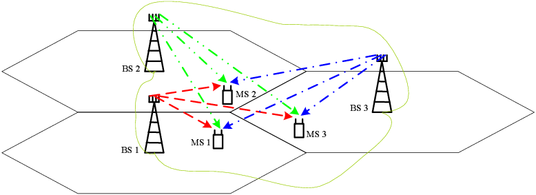
Without loss of generality, we assume that each BS has $n_{T}$ antennas and each MS has $n_{R}$ antennas⁴⁴ 4 Although we assume that the cooperating BSs and active MSs have homogeneous antenna configurations (i.e., every BS has $n_{T}$ transmit antennas, and every MS has $n_{R}$ receive antennas.), the proposed per-cell limited feedback mechanism can be directly extended to the cases with heterogeneous antenna configurations (i.e., different BSs and/or different MSs have different number of antennas.).. Assume limited feedback based block diagonalization (LF-BD) [7, 10] is employed for SDMA transmission in the network MIMO system, the downlink signal model can be written as,

where $\mathbf{y}_{k}\in\mathbb{C}^{n_{R}\times 1}$ is the received signal vector at the $k^{th}$ MS; $\mathbf{H}_{k}\in\mathbb{C}^{n_{R}\times Nn_{T}}$ denotes the aggregate CSI matrix of the $k^{th}$ MS; $\mathbf{\widehat{W}}_{k}\in\mathbb{C}^{Nn_{T}\times n_{R}}$ is the precoder for the $k^{th}$ MS, with $\mathbf{\widehat{W}}_{k}^{{\dagger}}\mathbf{\widehat{W}}_{k}=\mathbf{I}_{n_{R}}$; $\mathbf{P}_{k}=\frac{NP_{max}}{Kn_{R}}\mathbf{I}_{n_{R}}$ is the power allocation matrix for the $k^{th}$ MS, with $P_{max}$ representing the maximal transmit power of one BS; $\textbf{d}_{k}\in\mathbb{C}^{n_{R}\times 1}$ is the transmitted symbol vector intended for the $k^{th}$ MS, satisfying $\mathbb{E}\left\{\mathbf{d}_{k}\mathbf{d}_{k}^{{\dagger}}\right\}=\mathbf{I}_{n_{R}}$; $\mathbf{z}_{k}\in\mathbb{C}^{n_{R}\times 1}$ denotes the noise vector, with i.i.d. $\mathbb{CN}(0,\sigma^{2})$ entries, i.e., $\mathbb{E}\left\{\mathbf{z}_{k}\mathbf{z}_{k}^{{\dagger}}\right\}=\sigma^{2}\mathbf{I}_{n_{R}}$. In this paper, it is assumed that $Kn_{R}\leq Nn_{T}$.

For precoder design, LF-BD imposes the following conditions on $\mathbf{\widehat{W}}_{k}$ to eliminate CCI at the transmitter side [7, 10],

where $\mathbf{\widehat{H}}_{k}$ is the quantized aggregated CSI matrix of the $k^{th}$ MS (see equation (12)).

In the network MIMO system, the aggregate CSI matrix $\mathbf{H}_{k}$ seen by the $k^{th}$ MS can be partitioned into $N$ submatrices, i.e.,

where $\mathbf{H}_{k,n}\in\mathbb{C}^{n_{R}\times n_{T}}$ denotes the CSI matrix between the $n^{th}$ BS and the $k^{th}$ MS, which is commonly modeled as [22],

where $g_{k,n}\in\mathbb{R}_{+}$ denotes the path loss from the $n^{th}$ BS to $k^{th}$ MS; $s_{k,n}\in\mathbb{R}_{+}$ denotes the lognormal shadowing component; $\mathbf{H}_{k,n}^{(w)}\in\mathbb{C}^{n_{R}\times n_{T}}$ denotes a random matrix with i.i.d. $\mathbb{CN}(0,1)$ entries, i.e., the Rayleigh fading component.

Moreover, the aggregate CSI matrix $\mathbf{H}_{k}$ of the $k^{th}$ MS can be factorized as,

where $\mathbf{H}_{k}^{(w)}\in\mathbb{C}^{n_{R}\times Nn_{T}}$ denotes a random matrix with i.i.d. $\mathbb{CN}(0,1)$ entries; $\mathbf{G}_{k}\in\mathbb{R}^{Nn_{T}\times Nn_{T}}_{+}$ represents the large-scale fading component, which is given by,

where $\mathbf{1}_{n_{T}}$ equals to $\left[1\>1\>\cdots\>1\right]\in\mathbb{R}_{+}^{1\times n_{T}}$, and $diag(\mathbf{a})$ denotes a diagonal matrix with diagonal entries given by the elements of vector $\mathbf{a}$.

For downlink transmission with the LF-BD scheme, the essential information (i.e., users channel subspaces) required at the BSs side can be obtained through the codebook-based CSI feedback scheme. In a general codebook-based CSI feedback framework, the design metric⁵⁵ 5 For limited feedback based SDMA transmission, a widely adopted design metric for CSI feedback schemes is minimizing the inter-user interference, rather than maximizing the desired signal power [7, 10]. for minimizing the residual CCI is chordal distance[7, 10], which is defined as,

where $\mathbf{V}_{1},~\mathbf{V}_{2}\in\mathbb{C}^{Nn_{T}\times n_{R}}$ are two orthonormal matrices⁶⁶ 6 In this paper, an orthonormal matrix refers to a matrix with orthonormal columns.; and $\|\mathbf{A}\|_{F}$ denotes the Frobenius norm of matrix $\mathbf{A}$.

Without loss of generality, we assume the BS and MS share the same CSI quantization codebook, denoted by $\varphi$. The $J^{th}$ codeword in the codebook $\varphi$ is given by $\mathbf{V}_{J}$ and the cardinality of the codebook $\varphi$ is $2^{B}$, with $B$ representing the number of feedback-bits. In the conventional single-cell MIMO communications, the codeword index $J^{*}$ reported by the MS is generated through the minimization of the chordal distance between the quantization source $\mathbf{V}$ and the codedwords in the entire codebook $\varphi$. Mathematically,

The following assumptions are made through the rest of this paper. Firstly, all the MSs have perfect channel state information between the cooperative BSs and themselves. Secondly, the large-scale fading component $\mathbf{G}_{k}$ is known at all the BSs and MSs within the network. Thirdly, each MS shall feed back the CSI knowledge to the cooperative BSs through zero-delay error-free feedback links. In addition, flat block-fading MIMO channel is assumed.

In order to accommodate the dynamics of cooperating BSs and deal with the heterogeneous path loss effects, we propose to quantize $span\left\{\mathbf{H}_{k}^{(w)}\right\}$ with per-cell product codebooks, rather than quantizing $span\left\{\mathbf{H}_{k}\right\}$ directly, where $span\left\{\mathbf{A}\right\}$ denotes the row space of matrix $\mathbf{A}$. The proposed per-cell product codebook based CSI quantization procedure involves both MS side processing and BS side processing, i.e., codewords indices generation at the MS side and quantized aggregate CSI matrix reconstruction at the BS side. Denote the $N$ per-cell product codebooks as $\varphi_{1},\varphi_{2},\cdots,\varphi_{N}$, where $\varphi_{n}=\left\{\mathbf{V}\big|\mathbf{V}\in\mathbb{C}^{n_{T}\times n_{R}},\mathbf{V}^{{\dagger}}\mathbf{V}=\mathbf{I}_{n_{R}}\right\}$, with cardinality $2^{B_{k,n}}$, and the total number of per-user feedback-bits $B_{k}$ is given by $B_{k}=\sum_{n=1}^{N}B_{k,n}$. Note that the $N$ per-cell product codebooks could be identical. The proposed scalable limited feedback processing at the MS and the BS sides is summarized below:

Feedback Indices Generation (MS side): take the $k^{th}$ MS as an example. The feedback indices generation is a mapping from the normalized aggregated CSI matrix $\textbf{H}_{k}^{(w)}$ to the feedback indices $\big\{J_{k,1}^{*},$ $J_{k,2}^{*},\>\cdots,\>J_{k,N}^{*}\big\}$ corresponding to the $N$ per-cell product codebooks $\varphi_{1},\varphi_{2},\cdots,\varphi_{N}$.

• •

  Normalization: To handle the heterogeneous path loss effects, we first normalize the aggregate CSI matrix $\mathbf{H}_{k}$ by the large-scale fading component $\mathbf{G}_{k}$, i.e.,

  $\displaystyle\mathbf{H}_{k}^{(w)}=\mathbf{H}_{k}\mathbf{G}_{k}^{-1}.$

  (9)

• •

  Decomposition: Apply the standard singular value decomposition (SVD) [23] to the normalized CSI matrix $\mathbf{H}_{k}^{(w)}$, we have,

  	$\displaystyle\mathbf{H}_{k}^{(w)}$	$\displaystyle=$	$\displaystyle\mathbf{U}_{k}^{(w)}\left[\mathbf{S}_{k}^{(w)}\ \mathbf{0}_{n_{R}\times{Nn_{T}-n_{R}}}\right]\left[\mathbf{V}_{k}^{(w)}\ \mathbf{\tilde{V}}_{k}^{(w)}\right]^{{\dagger}}$		(10)
  		$\displaystyle=$	$\displaystyle\mathbf{U}_{k}^{(w)}\mathbf{S}_{k}^{(w)}\left[\mathbf{V}_{k}^{(w)}\right]^{{\dagger}}.$

• •

  Realtime Feedback Indices Selection: $\mathbf{V}_{k}^{(w)}$ is then mapped into $N$ per-cell product codebooks with indices $\big\{J_{k,1}^{*},$ $J_{k,2}^{*},\>\cdots,\>J_{k,N}^{*}\big\}$, and these codewords indices are fed back to the BSs via an error-free feedback link. The realtime indices generation is formulated as a combinatorial optimization in Section III-B.

Aggregate CSI Matrix Reconstruction and SDMA Precoder Computation (BS side): After collecting all the indices from the $K$ MSs, the BSs try to reconstruct the CSI matrices and compute the SDMA precoder from the $N$ codeword indices $\big\{J_{k,1}^{*},$ $J_{k,2}^{*},\>\cdots,\>J_{k,N}^{*}\big\}$.

• •

  Reconstruction: The indices $\left\{J_{k,1}^{*},J_{k,2}^{*},\cdots,J_{k,N}^{*}\right\}$ from the $k^{th}$ MS are used to construct a quantized version of $\mathbf{V}_{k}^{(w)}$ (denoted as $\mathbf{\widehat{V}}_{k}^{(w)}$), i.e.,

  $\displaystyle\mathbf{\widehat{V}}_{k}^{(w)}=\frac{1}{\sqrt{N}}\left[\mathbf{V}_{J_{k,1}^{*}}^{{\dagger}}\;\mathbf{V}_{J_{k,2}^{*}}^{{\dagger}}\;\cdots\;\mathbf{V}_{J_{k,N}^{*}}^{{\dagger}}\right]^{{\dagger}}.$

  (11)

• •

  Denormalization: $\mathbf{\widehat{V}}_{k}^{(w)}$ is used to construct the quantized aggregate CSI matrix $\mathbf{\widehat{H}}_{k}$ of the $k^{th}$ MS, which is given by,

  $\displaystyle\mathbf{\widehat{H}}_{k}=\left[\mathbf{\widehat{V}}_{k}^{(w)}\right]^{{\dagger}}\mathbf{G}_{k},~\forall~k=1,2,\cdots,K.$

  (12)

• •

  SDMA Precoder Computation: Apply the standard SVD to the quantized interference channel $\mathbf{\widehat{H}}_{-k}$ seen by the $k^{th}$ MS, we have,

  $\displaystyle\mathbf{\widehat{H}}_{-k}=\mathbf{\widehat{U}}_{-k}\mathbf{\widehat{S}}_{-k}\left[\mathbf{\widehat{V}}_{-k}\>\ \mathbf{\widetilde{\widehat{V}}}_{-k}\right]^{{\dagger}},$

  (13)

  where $\mathbf{\widehat{H}}_{-k}$ is given by,

  $\displaystyle\mathbf{\hat{H}}_{-k}=\left[\mathbf{\hat{H}^{{\dagger}}}_{1}\>\ \mathbf{\hat{H}^{{\dagger}}}_{2}\>\cdots\>\mathbf{\hat{H}^{{\dagger}}}_{k-1}\>\ \mathbf{\hat{H}^{{\dagger}}}_{k+1}\>\cdots\>\mathbf{\hat{H}^{{\dagger}}}_{K}\right]^{{\dagger}}.$

  (14)

  The SVD operation (13) generates an orthonormal basis of the right null space of $\mathbf{\widehat{H}}_{-k}$, i.e., $\mathbf{\widetilde{\widehat{V}}}_{-k}\in\mathbb{C}^{Nn_{T}\times n_{R}}$. We can set $\mathbf{\widehat{W}}_{k}=\mathbf{\widetilde{\widehat{V}}}_{-k}$, which satisfies equation (2).

As a summary, the proposed per-cell product codebook based limited feedback mechanism has the following advantages.

• •

  The proposed scheme relies on per-cell product codebooks, which are designed offline based on single-BS MIMO configurations. The proposed scheme is scalable w.r.t. any number of cooperating BSs.

• •

  Standard precoder codebooks (such as the Grassmannian codebook, Lloyd’s codebook, etc.) can be used in the proposed framework because the heterogeneous path loss issue is handled realtime in equation (9) and (12).

• •

  We could further exploit the special structure of $N$ per-cell product codebooks in the proposed framework to derive a low complexity feedback indices selection algorithm.

The feedback indices generation at the MS side is non-trivial, since it involves combinatorial search over the $N$ per-cell product codebooks. In the following, we shall first define the aggregate codeword for the $N$ per-cell product codebooks and then formulate the feedback indices generation problem as a chordal distance minimization problem between the aggregate-codeword and the quantization source.

By the definition of the aggregate-codeword, the feedback indices at $k^{th}$ MS side can be determined through the following optimization problem.

In the above proposed per-cell product codebook based limited feedback scheme, the aggregate codeword $\mathbf{\bar{V}}\left(J_{k,1},J_{k,2},\cdots,J_{k,N}\right)$ can be thought as a codeword in the product codebook $\varphi_{Per}=\varphi_{1}\otimes\varphi_{2}\otimes\cdots\otimes\varphi_{n}$, i.e.,

where $\mathbf{V}_{J_{k,n}}\in\varphi_{n}$, $\forall n=1,2,\cdots,N$. The product codebook $\varphi$ is important because it allows for a single codebook to be designed, and the real codebook that is used for CSI feedback is simply the Cartesian product of $N$ single cell codebooks $\left\{\varphi_{n}\right\}_{n=1}^{N}$.

Problem 1 belongs to the standard combinatorial search problem [24] and the optimal solution requires exhaustive search over the $N$ per-cell product codebooks, which has exponential complexity w.r.t. the number of feedback-bits $B_{k}$. However, in the practical communication systems, a MS may not be able to support such complicated operations. In order to address this issue, we shall propose a low-complexity searching algorithm, which exploit the per-cell product codebook structure and decomposes the searching process over the $N$ codebooks into the searching over $N$ sub-codebooks with reduced size. For illustration purpose, we shall first give the definition of sub-codebook.

Based on Definition 2, we can propose our low-complexity searching algorithm as well as complexity analysis in the following (see Algorithm 1 below).

We start with comparing the asymptotic performance of the proposed per-cell product codebook based limited feedback scheme and the joint-cell codebook approach. Denote $\varphi_{Joint}$ and $\Phi_{Joint}$ as a random joint-cell codebook and the collection of all possible random joint-cell codebooks, respectively. Similarly, denote $\varphi_{Per}$ and $\Phi_{Per}$ as a random product per-cell product codebook and the collection of all possible random product per-cell product codebooks, respectively, where a random product per-cell product codebook is defined as the Cartesian product of $N$ random per-cell product codebooks, i.e., $\varphi_{Per}=\varphi_{1}\otimes\varphi_{2}\otimes\cdots\otimes\varphi_{N}$. Let $\bar{D}_{k}\left(\Phi_{Joint}\right)$ and $\bar{D}_{k}\left(\Phi_{Per}\right)$ denote the average quantization distortion averaged over all possible random joint-cell codebooks and random per-cell product codebooks, respectively, which are defined as,

In order to show the efficiency of the proposed per-cell product codebook based limited feedback scheme, we shall establish the asymptotic optimality of the proposed limited feedback design w.r.t. the joint-cell codebook approach and summarize the main results in the following Lemma.

Within the framework of limit feedback study, the throughput loss due to CSI quantization is a common performance measure [8, 9, 10, 11]. In this paper, we extend the concept into network MIMO configuration and define per-user throughput loss $R_{k}^{Loss}$ as follows.

where CSIT is the abbreviation for Channel State Information at the Transmitter Side and LF is the abbreviation for Limited Feedback. Moreover,

with $\mathbf{W}_{k}$ denoting the percoder for the $k^{th}$ MS designed based on GCSI. Note that the residual CCI term in equation (28) is due to limited feedback effects, and the expectation operation is taken over Rayleigh fading and the lognormal shadowing effect, as well as the random per-cell product codebooks (for $R_{k}^{LF}$ only).   ∎

The following theorem quantifies the asymptotic per-user throughput loss of the proposed limited feedback scheme w.r.t. the network configuration $(n_{T},N,n_{R},K)$ , the per-user feedback-bits $B_{{}_{k}}$ and the path loss geometry $\big\{g_{k,1},g_{k,2},\cdots,g_{k,N}\big\}$, which consists of all the path losses between the $N$ cooperating BSs and the $k^{th}$ MS, and $\left\{g_{k,n}\right\}$ has been normalized to the weakest path so that $g_{k,n}\geq 1$.

Fig. 2 illustrates the per-user average throughput versus interference-free SNR. The simulation results show that, in the practical settings, the proposed per-cell product codebook based limited feedback scheme can achieve $95\%\sim 97\%$ the performance of the joint-cell codebook approach. Moreover, the proposed scheme achieves much better throughput compared with Baseline 2 (Givens rotation approach with doubled number of bits for limited feedback) and Baseline 3 (Givens rotation approach). This is because the Givens rotation approach has quite low feedback efficiency due to two-dimensional vector quantization, compared with matrix quantization in the codebook-based approach.

In this section, we study the performance-complexity tradeoff of the low-complexity ISA. Here, performance is measured in terms of per-user ergodic capacity, and complexity is measured in terms of the number of codewords that are searched for generating the codewords indices. As stated in section III-C, the parameters $\delta_{n}~(n=1,2,\cdots,N)$ determine the tradeoff between performance and complexity of algorithm 1.

Fig. 3 shows the performance-complexity tradeoff with different choices of $\delta_{n}$, where we set $\delta_{n}$ to the same value for all $n$. The complexity numbers shown in the figure denote the relative complexity with respect to the exhaustive search method with original codebooks, i.e.,

As shown in the figure, with $\delta_{n}=0.9$, the low-complexity ISA can achieve $92\%$ the performance of the exhaustive search approach, with only $1\%$ complexity of the exhaustive search. With larger $\delta_{n}$, algorithm 1 can achieve better performance at the cost of higher computational complexity, and vice versa.

In this section, we shall compare the analytical results stated in Corollary 1 and Corollary 2 with numerical results, and demonstrate the validity of those analytical studies.

Fig. 4 shows the simulation results for GCSI case, per-cell product codebook limited feedback with scaling feedback-bits and fixed feedback-bits. For the per-cell product codebook based limited feedback with scaling feedback-bits, we set $\varepsilon=1$ and let the feedback-bits scale according to equation (30). Compared with GCSI case, about 0.5 (bits per channel use) throughput loss is achieved with scaling-feedback.

Fig. 5 shows the performance of the proposed per-cell product codebook based limited feedback scheme in interference limited regime, with different number of feedback-bits per BS (i.e., $\frac{B_{k}}{N}$). We can see that the per-user ergodic capacity scales linearly w.r.t. feedback-bits per BS under all system configurations $\left(n_{T},N,n_{R},K\right)$. The simulation results shown in Fig. 5 match the analytical results stated in Corollary 2.

References

- [1] M. Karakayali, G. Foschini, and R. Valenzuela, “Network coordination for spectrally efficient communications in cellular systems,” IEEE Wireless Commun. Mag., vol. 13, no. 4, pp. 56–61, Aug. 2006.
- [2] G. Foschini, K. Karakayali, and R. Valenzuela, “Coordinating multiple antenna cellular networks to achieve enormous spectral efficiency,” IEE Proceedings of Communications, vol. 153, no. 4, pp. 548–555, Aug. 2006.
- [3] J. Andrews, W. Choi, and R. Heath, “Overcoming interference in spatial multiplexing MIMO cellular networks,” IEEE Wireless Commun. Mag., vol. 14, no. 6, pp. 95–104, Dec. 2007.
- [4] S. Jing, D. N. C. Tse, J. B. Soriaga, J. Hou, J. E. Smee, and R. Padovani, “Multicell downlink capacity with coordinated processing,” EURASIP J. Wirel. Commun. Netw., vol. 2008, no. 5, pp. 1–19, Jan. 2008.
- [5] L.-U. Choi and R. D. Murch, “A transmit pre-processing technique for multi-user MIMO systems using a decomposition approach,” IEEE Trans. Wireless Commun., vol. 3, no. 1, pp. 20–24, Jan. 2004.
- [6] Q. Spencer, A. Swindlehurst, and M. Haardt, “Zero-forcing methods for downlink spatial multiplexing in multiuser MIMO channels,” IEEE Trans. Signal Process., vol. 52, no. 2, pp. 461–471, Feb. 2004.
- [7] C. WANG, Adaptive downlink multi-user MIMO wireless systems. PhD dissertation, Hong Kong University of Science and Technology, Aug. 2007.
- [8] N. Jindal, “MIMO broadcast channels with finite-rate feedback,” IEEE Trans. Inf. Theory, vol. 52, no. 11, pp. 5045–5060, Nov. 2006.
- [9] T. Yoo, N. Jindal, and A. Goldsmith, “Multi-antenna downlink channels with limited feedback and user selection,” IEEE J. Sel. Areas Commun., vol. 25, no. 7, pp. 1478–1491, 2007.
- [10] N. Ravindran and N. Jindal, “Limited feedback-based block diagonalization for the MIMO broadcast channel,” IEEE J. Sel. Areas Commun., vol. 26, no. 8, pp. 1473–1482, Oct. 2008.
- [11] K. Huang, J. Andrews, and R. Heath, “Performance of orthogonal beamforming for SDMA with limited feedback,” IEEE Trans. Veh. Technol., vol. 58, no. 1, pp. 152–164, Jan. 2009.
- [12] M. Trivellato, H. Huang, and F. Boccardi, “Antenna combining and codebook design for the MIMO broadcast channel with limited feedback,” in Asilomar Conference on Signals, Systems and Computers, 2007, Pacific Grove, USA, nov. 2007, pp. 302 –308.
- [13] M. Trivellato, F. Boccardi, and H. Huang, “On transceiver design and channel quantization for downlink multiuser MIMO systems with limited feedback,” IEEE J. Sel. Areas Commun., vol. 26, no. 8, pp. 1494–1504, 2008.
- [14] J. H. Kim, W. Zirwas, and M. Haardt, “Efficient feedback via subspace-based channel quantization for distributed cooperative antenna systems with temporally correlated channels,” EURASIP J. Adv. Signal Process, vol. 2008, no. 2, pp. 1–13, Jan. 2008.
- [15] L. Thiele, M. Schellmann, T. Wirth, and V. Jungnickel, “Cooperative Multi-User MIMO based on Reduced Feedback in Downlink OFDM Systems,” in 42nd Asilomar Conference on Signals, Systems and Computers, Monterey, USA, Oct. 2008.
- [16] D. J. Love and R. W. H. Jr., “Limited feedback unitary precoding for spatial multiplexing systems,” IEEE Trans. Inf. Theory, vol. 51, no. 7, pp. 2967–2976, Aug. 2005.
- [17] B. Mondal, S. Dutta, and R. W. Heath, “Quantization on the Grassmann manifold,” IEEE Trans. Signal Process., vol. 55, no. 8, pp. 4208–4216, Aug. 2008.
- [18] W. Dai, Y. Liu, and B. Rider, “Quantization bounds on Grassmann manifolds and and applications to MIMO communications,” IEEE Trans. Inf. Theory, vol. 54, no. 3, pp. 1108–1123, Mar. 2008.
- [19] J. C. Roh and B. Rao, “An efficient feedback method for MIMO systems with slowly time-varying channels,” vol. 2, 2004, pp. 760–764 Vol.2.
- [20] M. A. Sadrabadi, A. K. Khandani, and F. Lahouti, “Channel feedback quantization for high data rate MIMO systems,” IEEE Trans. Wireless Commun., vol. 5, no. 12, pp. 3335–3338, Dec. 2006.
- [21] H. Long, W. Wang, H. Zhao, and K. Zheng, “Precoding vector distribution under spatial correlated channel and nonuniform codebook design,” in IEEE ICC’08, May 2008, pp. 4506–4510.
- [22] H. Zhang and H. Dai, “Cochannel interference mitigation and cooperative processing in downlink multicell multiuser MIMO networks,” EURASIP J. Wirel. Commun. Netw., vol. 2004, no. 2, 2004.
- [23] D. Tse and P. Viswanath, Fundamentals Of Wireless Communication. Cambridge University Press, 2005.
- [24] C. H. Papadimitriou and K. Steiglitz, Combinatorial Optimization: Algorithms and Complexity. Dover Publications, 1998.
- [25] IEEE 802.16m evaluation methodology document. IEEE 802.16m-08/004r4. [Online]. Available: http://www.ieee802.org/16/tgm/
- [26] P. K. Sen and J. M. Singer, Large Sample Methods in Statistics: An Introduction with Applications. Chapman & Hall, New York, 1993.