Search for Acoustic Signals from Ultra-High Energy Neutrinos
in 1500 km3 of Sea Water
Abstract
An underwater acoustic sensor array spanning 1500 km3 is used to search for cosmic-ray neutrinos of ultra-high energies (UHE, 1018 eV). Approximately 328 million triggers accumulated over an integrated 130 days of data taking are analysed. The sensitivity of the experiment is determined from a Monte Carlo simulation of the array using recorded noise conditions and expected waveforms. Two events are found to have properties compatible with showers in the energy range eV5 eV and eV5 eV. Since the understanding of impulsive backgrounds is limited, a flux upper limit is set providing the most sensitive limit on UHE neutrinos using the acoustic technique.
pacs
95.85.Ry, 43.60.Bf, 14.60.LmI INTRODUCTION
In the last few decades considerable attention has been devoted to understanding the origin, acceleration mechanisms, flux, and composition of the highest energy cosmic rays. Neutrinos are thought to play an important role at ultra-high energies (UHE, E1018 eV). Different mechanisms are being explored to probe the extremely small neutrino flux ( 1 km-2 yr-1) expected in this regime. In the last decade, feasibility studies for acoustic UHE neutrino detectors have been initiated in large natural bodies of water, ice and salt. The advantage to this technique is the possibility of building very large arrays (thousands of km3) with sparse microphones, thanks to the large attenuation length of sound at the appropriate frequencies in these media. The Study of Acoustic Ultra-high Energy Neutrino Detection (SAUND) phase II is the first experiment to read out hydrophones undersea for the purpose of detecting UHE neutrinos using such an expansive array (1500 km3), and follows the first phase [1] where 15 km3 were read out at the same site.
Acoustic radiation is produced from the volume expansion caused by the heating of the medium where the neutrino interacts and produces a shower. Theoretical models [2] and experimental measurements [3] show that the signature of this event is a single bipolar pulse, with acoustic energy concentrated around 10 kHz. Noise conditions measured by SAUND II have been studied in detail [4]. The analysis revealed that although the ambient noise correlates well with surface wind speeds, at higher frequencies the spectrum rolled off much faster than the expected power law due to the large depth of the hydrophones. The expected noise profile was parametrized and a good agreement was observed when compared to measured profiles.
Full data processing of pulse shapes, analysis of multi-hydrophone coincidences, and other techniques intended to reject background are reported here, along with a UHE neutrino flux limit set by a detailed simulation of the full experimental procedure.
II THE SAUND II EXPERIMENT
The second phase of SAUND (SAUND II) employs a large hydrophone array at the US Navy’s Atlantic Undersea Test and Evaluation Center (AUTEC) located at the Tongue of the Ocean (TOTO) in the Bahamas. SAUND II is currently the largest test for the feasibility of acoustic ultra-high-energy neutrino detection. This program follows a general study of the expected performance [5], and a first experimental phase (SAUND I) using seven hydrophones [1]. Since then, the US Navy has upgraded the hydrophones and the readout system of the array. SAUND II uses 49 of these hydrophones with digitized signals transmitted to shore over optical fibers. The array spans an area of km km with spacing of 3 to 5 km. Hydrophones are mounted 5.2 m above the ocean floor, at depths between 1340 and 1880 m. Fig. 1 shows the configuration and the topography of the ocean floor. Hydrophones are omnidirectional with a flat response (within 5 dB) at the frequencies considered. The gains of the 49 channels coincide to within 1 dB. Analog signals are regenerated at the shore station from the digital data (by the US Navy for their backwards compatibility) and fed to the SAUND II data acquisition (DAQ) system that re-digitizes them at 156 kHz. Since low frequencies are not relevant for SAUND II, a hardware high-pass RC filter is applied to the analog data with a 3 dB point at 100 Hz.

A DAQ program with real-time analysis running on seven PCs records candidate neutrino events using a matched filter with the bipolar response function shown in Fig. 2. Because the phase response of the electronic system is unknown, SAUND II only considers the absolute value of the matched filter. Once per minute, the trigger threshold on each hydrophone is adjusted independently to a value that would have acquired 20 triggers/min in the previous minute. This differs from the SAUND I algorithm which only allowed thresholds to move up or down by a fixed step size. Each hydrophone triggers independently, and a 1 ms time series of only the triggered hydrophone is recorded. In addition, every minute the threshold on each hydrophone is recorded. The noise conditions in the form of a power spectral density (PSD) and root mean square (RMS) are recorded every 5 s and 0.1 s respectively for each hydrophone.

The SAUND II DAQ system consists of seven National Instruments cards (NI-PCI-MIO-64)and eight PCs of which seven are dedicated to data acquisition and one for controlling the entire system. It also includes a front-end module with hardware high-pass filters and an IRIG timing signal distributor that connects to each of the cards. The NI ADC cards are controlled by COMEDI [6], and the DAQ software uses KiNOKO [7].
By agreement with the US Navy, the SAUND II data acquisition system records data only when the array is not otherwise in use. From July 2006 to September 2007, the system ran under stable conditions for a total integrated time of more than 130 days as shown in Fig. 3.

Thresholds used in SAUND II are compared to those used in SAUND I in Fig. 4. Since the same region of sea is measured over several seasons, ambient noise in both experiments is expected to produce similar distributions. However, SAUND II measures lower levels of adaptive thresholds overall. This is due to a better electrical noise performance of the new array, owing to the absence of long coaxial cables and digital transmission of signals on fibers.

III DATA ANALYSIS
Table 1 shows the total number of triggers accumulated and the size of the remaining data set after selection cuts are applied. Cuts 1 through 4 are applied on single-hydrophone triggers. After the source position in the ocean is triangulated using time difference of arrival, characteristics of these multi-hydrophone acoustic events are used on further cuts to test their consistency with expected properties of neutrino showers. In order to establish data analysis cuts that are minimally biased, an 8% subset of data was initially used to establish the data reduction cuts. Because the noise environment can vary greatly depending on time of day and season, the subset was selected carefully to have a random distribution in time. Cuts 1 through 3 result from analysing the 8% data alone. Once the full data was processed, it was found that some triggers are artificially generated by cross-talk between read-out channels. This effect was not discovered in the reduced data set as it affects a very small fraction of triggers. Therefore, parameters for cuts 4 to 7 have been modified on the full data set to eliminate triggers caused by cross-talk while maintaining efficiency for neutrino showers. The method used to validate this procedure is described in section IV.
In Table 1, the number of Online Triggers is the total number of triggers recorded by the online DAQ system in all hydrophones. Minutes of individual hydrophones with high threshold (0.04), high trigger rate (500 triggers/min compared to the target 20 triggers/min set by the DAQ), high trigger rate on a nearest neighbor, or man-made noise in the water are excluded to select Quality Triggers. Man-made noise can contaminate large parts of the array, and can be identified by narrow-band frequencies continuously dominating a wide area of hydrophones. This condition occurred a total integrated time of 9 min. Furthermore, data periods where the input cables appear to be disconnected are also removed. Such periods have unphysical, low noise levels, and are attributed to Navy personnel disconnecting individual cables for diagnosing problems in their system. One hydrophone had to be excluded entirely due to the majority of data belonging to this condition. For the remaining 48 hydrophones, this condition excludes 6% of integrated livetime.
| Single-phone | ||
| Cut | Triggers | Events |
| 1. Online Triggers | 327.9M | — |
| 2. Quality Triggers | 146.7M | — |
| 3. Waveform Selection | 2,814,545 | — |
| 4. Single Phone Rate | 2,562,047 | — |
| 5. Triangulation | 6,605 | 4,995 |
| 6. Isolated Event | 1,227 | 320 |
| 7. Radiation Pattern | 8 | 2 |
Waveform Selection is used to further reduce background triggers. For each trigger, the online data acquisition system records a 1 ms waveform centered around the time of trigger. The absolute value of the matched-filter time series, , is calculated using the response function shown in Fig. 2 for each time series. The Waveform Selection cut is based on two parameters from this time series: the peak area ratio (PAR) and the Gaussian width (GW). The PAR is obtained by dividing the value of obtained at the time of trigger by the integral of in the 1 ms window; PAR= where is the time of trigger. This quantity measures the significance of the trigger compared to its surrounding times. The GW is obtained by smoothing the time series of to obtain the envelope shape, fitting this to a Gaussian, and extracting its width. For neutrino-induced signals, the width should be 40 s. Many marine animals vocalize around frequencies of interest for this work. However, the signals originating from such sources tend to have a larger GW value. Fig. 5 compares these parameters for two triggers from the data set. The distribution of these parameters and the cut region where neutrino showers are expected are shown in Fig. 6. Triggers consisting of at least one data sample that saturate the ADC at 3.15 Pa bypass this cut and are kept regardless of the PAR and GW parameters.


The Single Phone Rate cut removes surviving triggers that occur on a single hydrophone clustered in time. Triggers accompanied by 10 or more triggers in any 5 s window are removed. In addition, triggers that occur less that 10 ms from each other are also removed. These rates are significantly higher than the 20 triggers/min target trigger rate set by the DAQ. Diffused, steady state UHE neutrinos are not expected to arrive and interact in bursts, so the removal of clustered triggers on single hydrophones only affects the livetime. Marine animals and artificial sources are usually responsible for such trigger patterns.
With the remaining triggers Triangulation is performed. The 6,605 triggers produce 4,995 source locations in the ocean by requiring four hydrophones to have the appropriate difference in arrival times. The time difference of arrival method used is described in [1] and includes the effects of the depth-dependent speed of sound in the ocean. Only hydrophones that are within 8 km of the hydrophone of earliest arrival time are considered for each event. For each event, a local rectangular coordinate system tangent to the Earth surface, centered around the earliest arrival-time hydrophone is used. High rates of trigger on a single hydrophone in the coincidence time window (8 s) produce combinatorics such that a single trigger can be involved in multiple events. However, by further excluding events that trigger the same hydrophone within a minute of each other, only 320 time Isolated Events survive.
Since acoustic radiation from neutrino showers is not expected to be emitted spherically, but rather in a disk-like shape orthogonal to the direction of the shower [2, 5], only showers of certain energy and orientation combinations can produce pulses capable of triggering all four hydrophones from the triangulated event location. This geometric constraint utilises the thresholds set at the time of the event, and only selects showers that are capable of triggering all four hydrophones with its acoustic radiation. However, not only does the radiation need to exceed the thresholds, but estimated pressure amplitudes must also be observed in the recorded waveforms. Only two events have observed pressures matching or exceeding those expected by geometrically possible showers, and pass the Radiation Pattern cut. A metric, , quantifies the ratio of pressure missing in the recorded peak pressure, , from the estimated peak amplitudes, .
| (1) |
where
| (2) |
Since is defined as the pressure missing, it is set to zero for waveforms meeting or exceeding estimated pressure amplitudes. is calculated for a dense grid of shower energy-orientation combinations for each event. Fig. 7 shows the minimum values obtained by considering all possible , , and configurations for each of the 320 events. 244 events did not have possible showers with any direction and energy less than 51024 eV that fit the geometric constraint, and are assigned .

Events with pass the Radiation Pattern cut. The two events that pass require the shower energy to be eV51024 eV and eV5 eV in order to be consistent with measured thresholds and peak pressures.
IV EFFICIENCY AND SENSITIVITY ESTIMATES
The SAUND II detector is large enough to observe very different noise environments in different parts of the array. Therefore, the Quality Triggers cut described above removes livetime from single hydrophones minute-by-minute. Hence the configuration of enabled hydrophones is a complex pattern that varies from one minute to the next. To properly account for this, and to estimate the efficiency of the analysis cuts described above, neutrino events of different energies are generated by Monte Carlo simulation and injected randomly into the SAUND II livetime.
The Monte Carlo study uses 66M simulated neutrino events generated with the following distribution in zenith angle and depth ,
| (3) |
where is the energy-dependent interaction length given by . is assumed to scale with energy as [8], is the density of sea water, and is Avogadro’s number. The events are generated uniformly in the azimuthal angle as well as in latitude and longitude, in a 35 km57 km rectangular area completely encompassing the SAUND II array. The closest hydrophone-boundary distance is 3 km. The fraction of neutrino energy deposited into the hadron shower, , is generated with the distribution
| (4) |
where and [9]. The hadron shower energy is obtained by . We assume the same distributions for all flavors of neutrinos. Ray tracing is performed between each hydrophone-event pair including the effects of sound speed variation in the ocean to obtain arrival times. The topography of the ocean floor is also considered. This produces some volume of ocean from where no rays can reach the hydrophones without intersecting with the ocean floor. An acoustic pulse is generated for each hydrophone-event pair using shower parameters [10] and attenuation. For each event, a time of occurrence is assigned with a distribution that is uniformly random in the SAUND II livetime. This allows the assignment of realistic noise conditions from the data to each hydrophone in each event.
Trigger candidates are then passed through the cuts in Table 1. First the matched filter values of the Monte Carlo candidate triggers are compared to the threshold set at the occurrence time and hydrophone. The Quality Triggers cut keeps only the triggers that were assigned a timestamp with good run conditions, while the Waveform Selection cut discriminates on simulated pulse shapes with added noise.
The Single Phone Rate cut which is based on the rate of triggers on a single hydrophone can be affected by cross-talk. When a triggered waveform on one hydrophone produces cross-talk on other hydrophones that are also triggered, additional artificial triggers are created. The false increase in the trigger rate during this short period of time can affect the Single Phone Rate cut. To account for these situations, cross-talk triggers are generated by using the arrival times of surviving triggers and creating additional triggers on hydrophones within 8 km (electronic cross-talk is instantaneous compared to both the speed of sound in water and the sampling frequency of the ADC cards). The Single Phone Rate cut and Triangulation are then performed including these false triggers. None of the artificial cross-talk triggers were found to generate events. The parameters used for the Single Phone Rate cut were chosen to minimize the rejection of true events in the presence of cross-talk.
The Isolated Event cut creates deadtime that is much less than 1% of the integrated livetime. Finally Radiation Pattern fitting is performed to confirm that the metric , as shown in Fig. 7.
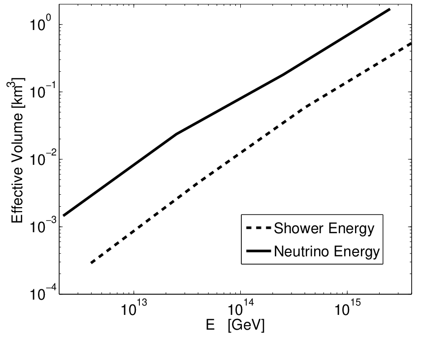
The efficiency of the SAUND II detector, , is obtained at each decade of neutrino energy and shower energy. The effective volume, , where is the volume in which Monte Carlo events are generated, is shown in Fig. 8. Using the model-independent method described in [11], the sensitivity for UHE neutrino flux at different neutrino and hadron shower energies is plotted in Fig. 9 using a 90% confidence interval and assuming events remaining after cuts.

V DISCUSSION AND RESULTS
In order to formalize the SAUND II results, the two events surviving all cuts must be accounted for. The four triggers associated with each event are shown in Fig. 10 and Fig. 11.


Further analysis capable of confirming the remaining two events as background or signal will require better understanding of the detector. Because the phase response of the system is unknown, the phase information of the triggered pulses is not utilised to discriminate events. Thus the event shown in Fig. 10 contains bipolar pulses with flipped phases, which are probably inconsistent as waveforms due to the same acoustic source. Apart from the phase, three of the four waveforms in Fig. 10 have similar high-amplitude bipolar pulses followed by a few more cycles of oscillation, while the fourth waveform on the top right has a much lower signal-to-noise. Since the probability of triangulating random arrival times to a single source location is extremely low, and since the four triggers are of order 100 ms to seconds apart, the origin of this event is assumed to be acoustic despite its peculiar features. Furthermore, the three high-amplitude waveforms are similar to a type of background repeatedly seen in the SAUND II data set. All but the waveforms in Fig. 10 are eliminated due to their high repetition rate during their occasional bursts. The triggers in Fig. 10, however, occur isolated in time and cannot be eliminated in such way.
As discussed in [12], the phase response of a hydrophone read-out system can distort bipolar pulses into more cycles, creating multi-polar oscillation signals. For this reason, the Waveform Selection cut does not define or utilize the number of cycles of oscillation. Thus some of the waveforms shown in Fig. 11 are not clearly bipolar. In addition, because many triggers occur with amplitudes that are not significantly higher than the noise level, it is difficult to define how many peaks constitute a signal. This effect also compounds the difficulty in phase matching bipolar pulses.
Given the a posteriori observation made on two events, and the inability to perform a meaningful statistical analysis with such a small data set, an upper limit on the flux is set. Since the knowledge of impulsive backgrounds is incomplete, an upper limit with statistical significance on neutrino flux alone cannot be derived. Nevertheless, a conservative limit can be obtained by assuming that the two events are due to signal, and no other background is present. Following the treatment in [11],
| (5) |
where is the expected number of events, is the sensitivity of the experiment at different energies, and is the UHE neutrino flux. For a 90% confidence level,
| (6) |
where is the 90% Poisson confidence interval upper limit of event detection. At each neutrino energy bin, is calculated for different shower energy ranges . For shower energy ranges – eV and – eV, is used, making the upper bound . For other shower energy ranges, is used, making the upper bound . At each neutrino energy, a weighted average is calculated using
| (7) |
where is the number of neutrinos that will produce a shower in the energy range when neutrinos are generated at neutrino-energy range . The weighted average gives at each neutrino energy, and is used to set a flux limit
| (8) |
The limit obtained by this method along with other experimental limits are plotted in Fig. 12.

VI CONCLUSION
The main factors contributing to the difference in sensitivities of SAUND I and SAUND II are volume, threshold, and hydrophone spacing. While SAUND II is advantageous in the first two factors, its sensitivity is limited by the larger hydrophone spacing. In both arrays, hydrophones are mounted on the ocean floor, resulting in a mostly flat, two dimensional geometry which severely limits the sensitivity to the emission properties of showers, as already discussed in [1].
Unambiguously identifying rare UHE neutrinos from either acoustic or radio signals in huge naturally occurring bodies subject to varying and poorly understood backgrounds is very difficult. Combining multiple techniques in a hybrid array featuring acoustic, radio, and/or optical detectors makes it possible to identify neutrinos by detecting two signals that have very different production and propagation mechanisms as well as backgrounds. One possible array has been simulated in [18]. In the absence of such arrays, it is important to understand and identify backgrounds. The extensive study of the ambient noise condition using SAUND II data [4] revealed that deep oceans are quieter than usually assumed at the high acoustic frequencies of interest. A model of such noise and a parametrization useful for ultra-high energy neutrino detection was developed. In executing a full analysis capable of detecting very rare events consistent with shower-induced signals, it was found that transient noise originating from discrete acoustic sources in the water causes the main limitation. A powerful cut, the Radiation Pattern cut, was developed to distinguish the geometry of emission to cope with such transient events. This cut will be significantly more effective when used with arrays of hydrophones arranged in all three dimensions. From such arrays, more information regarding the geometry of the emission lobe can be extracted.
Acknowledgements.
We would like to thank the US Navy and, in particular, D. Deveau and T. Kelly-Bissonnette for their hospitality and help at the AUTEC site. We are grateful to D. Kapolka (Naval Postgraduate School) and S. Waldman (Massachusetts Institute of Technology) for sharing their insights and expertise, and J. Kerwin, K. Montag, and S. Wilson for their contributions through Summer Research College at Stanford University. J. V. is supported by a Kavli Fellowship from the Kavli Foundation. This work was supported, in part, by NSF grant PHY-0457273.References
- [1] J. Vandenbroucke, G. Gratta, and N. Lehtinen, ApJ 621, 301 (2004).
- [2] J. G. Learned, Phys. Rev. D 19, 3293 (1979).
- [3] L. Sulak, T. Armstrong, H. Baranger, M. Bregman, M. Levi, D. Mael, J. Strait, T. Bowen, A. E. Pifer, P. A. Polakos, et al., Nucl. Instrum. Methods 161, 203 (1979).
- [4] N. Kurahashi and G. Gratta, Phys. Rev. D 78, 092001 (2008).
- [5] N. G. Lehtinen, S. Adam, G. Gratta, T. K. Berger, and M. J. Buckingham, Astropart. Phys. 17, 279 (2002).
- [6] COMEDI - Control and Measurement Device Interface, http://www.comedi.org, open soure drivers, tools, and libraries for data acquisition plug-in boards.
- [7] KiNOKO, http://www.awa.tohoku.ac.jp/~sanshiro/kinoko-e/, a general purpose online data acquisition system designed for high-energy physics experiments. Primarily developed for the KamLAND experiment.
- [8] R. Gandhi et al., Phys. Rev. D 39, 093009 (1998).
- [9] A. R. Beresnyak (2004), eprint arXiv:0310295.
- [10] J. Alvarez-Muniz and E. Zas, Phys. Lett. B 434, 396 (1998).
- [11] N. G. Lehtinen et al., Phys. Rev. D 69, 013008 (2004).
- [12] S. Danaher et al., J. Phys.: Conf. Ser. 81, 012011 (2007).
- [13] P. W. Gorham et al., Phys. Rev. Lett. 93, 041101 (2004).
- [14] P. W. Gorham et al., Phys. Rev. D 82, 022004 (2010).
- [15] C. W. James et al., Phys. Rev. D 81, 042003 (2010).
- [16] O. Scholten et al., Phys. Rev. Lett. 103, 191301 (2009).
- [17] S. Buitink et al., A&A (2010), preprint doi 10.1051/0004-6361/201014104, eprint arXiv:1004.027v1.
- [18] J. Vandenbroucke et al., J. Phys.: Conf. Ser. 60, 288 (2007).