Chemical signatures of the first star clusters in the Universe
Abstract
The chemical abundance patterns of the oldest stars in the Galaxy are expected to contain residual signatures of the first stars in the early universe. Numerous studies attempt to explain the intrinsic abundance scatter observed in some metal-poor populations in terms of chemical inhomogeneities dispersed throughout the early Galactic medium due to discrete enrichment events. Just how the complex data and models are to be interpreted with respect to “progenitor yields” remains an open question. Here we show that stochastic chemical evolution models to date have overlooked a crucial fact. Essentially all stars today are born in highly homogeneous star clusters and it is likely that this was also true at early times. When this ingredient is included, the overall scatter in the abundance plane [Fe/H] vs. [X/Fe] (space), where X is a nucleosynthetic element, can be much less than derived from earlier models. Moreover, for moderately flat cluster mass functions (), and/or for mass functions with a high mass cut-off ( M⊙), stars exhibit a high degree of clumping in space that can be identified even in relatively small data samples. Since stellar abundances can be modified by mass transfer in close binaries, clustered signatures are essential for deriving the yields of the first supernovae. We present a statistical test to determine whether a given set of observations exhibit such behaviour. Our initial work focusses on two dimensions in space, but we show that the clustering signal can be greatly enhanced by additional abundance axes. The proposed experiment will be challenging on existing 8-10m telescopes, but relatively straightforward for a multi-object echelle spectrograph mounted on a 25-40m telescope.
Subject headings
Galaxy – dwarf galaxies – stellar populations – star clusters – elemental abundancesI. Introduction
The Galactic stellar halo is a vast ancient repository that takes us back to a time when dark matter collapsed into bound structures and the Galaxy was seeded for the first time. Helmi (2008) and Tolstoy, Hill & Tosi (2009) provide excellent overviews of the many stellar systems and fragments that inhabit the halo. These include field halo stars (Christlieb et al 2002; Cayrel et al 2004; Frebel et al 2005; Cohen et al 2007), globular clusters (Gratton, Sneden & Carretta 2004), dwarf spheroidals (Mateo 1999; Venn et al 2004), ultra-faint dwarf galaxies (Simon & Geha 2007; Kirby et al 2008), stellar streams (Ibata et al 1995; Chou et al 2010), stellar associations (Walsh et al 2007) and satellites to dwarf galaxies (Coleman et al 2004; Belokurov et al 2009). Already the chemical information arising from the most metal-poor stars is very difficult to unravel (Nomoto et al 2005; Kirby et al 2008). We have barely begun to understand what these systems are telling us about the sequence of events that led to the Galaxy (McWilliam, Simon & Frebel 2009; Freeman & Bland-Hawthorn 2002).
The first stars were unique to their time. The first stellar generations changed the universe in many ways, in particular, the chemical properties and the equation of state of the intergalactic medium. But at present there are many unknowns. Did the first stars form in isolation or in groups? Were relatively few massive stars responsible for reionization or was it triggered by the collective effect of massive star clusters? Just what are the processes that govern star formation at extremely low metallicity? Is this exclusively the domain of the most massive stars, or can substantial intermediate and low mass stars form (Tsuribe & Omukai 2006, 2008; Clark, Glover & Klessen 2008)? In other words, did stellar populations observable today exist before reionization (Tumlinson 2010; Okrochov & Tumlinson 2010)? The first star clusters are of great interest in that they shed light on star formation processes in the early universe (Bromm, Coppi & Larson 2002; Abel et al 2002). There are few if any reliable constraints at the present time.
One of the most interesting developments in recent years is the simultaneous measurement of many elemental abundances for individual metal-poor halo stars or groups of stars (e.g. Beers & Christlieb 2005). Some of these elements, but not all, exhibit intrinsic scatter in the abundance plane [Fe/H] vs. [X/Fe] that exceeds the measurement errors. While the scatter is particularly apparent in halo stars (e.g. Roederer et al 2009), evidence is now emerging that star-to-star abundance variations exist in dwarf galaxies as well (Fulbright, Rich & Castro 2004; Koch et al 2008; Feltzing et al 2009). The observed scatter is likely to increase now that metal poor stars are now detected below [Fe/H] -3 (Norris et al 2009; Starkenburg et al 2010; Simon et al 2010; Frebel, Kirby & Simon 2010).
This has led numerous researchers to argue that the scatter in [X/Fe] is a tracer of an ancient inhomogeneous medium (e.g. Audouze & Silk 1995; Ryan, Norris & Beers 1996; McWilliam 1997; Ishimaru & Wanajo 1999). If this interpretation is correct, we would expect that a subset of these stars is telling us something fundamental about the first stars and their yields. But not all of the stars are providing us with an unambiguous “reading” of the early enrichment of the primordial interstellar gas. For example, a significant fraction of extremely metal poor stars appear to have undergone mass transfer with a companion (Ryan et al 2005; Lucatello et al 2005) which undermines any attempt at inferring the progenitor yields for elements such as CNO and elements. Binarity may partly explain why the elemental abundances of the most metal poor stars defy a clear explanation at the present time (Joggerst et al 2010; McWilliam et al 2009).
We now incorporate a missing ingredient into existing models of stochastic chemical evolution. In the present-day universe, most stars are born in a single burst within compact clusters and stellar fragments, rather than in isolation. This fact is well established in the local universe (Lada & Lada 2003) and is likely to be true at the time of the first stars (Clark et al 2008). Cluster formation has an important consequence for the distribution of stars in the abundance plane. De Silva et al (2006, 2007a,b) have shown that both old ( 10 Gyr) and intermediate-age ( Gyr) open clusters are chemically homogeneous to a high degree ([Fe/H] dex). The open cluster Tombaugh 2 was thought to be a rare example of a chemically inhomogeneous open cluster (Frinchaboy et al 2008), but this is contradicted by a new study that finds the stellar population to be highly homogeneous ([Fe/H] dex; Villanova et al 2010). Apart from a few light elements, the same holds true for globular clusters (Gratton et al 2004), although some systems (e.g. Cen) show evidence for more than one burst of star formation. Interestingly, even moving groups can show the same signature of chemical homogeneity (De Silva et al 2007a; Chou et al 2010; Bubar & King 2010).
Bland-Hawthorn, Krumholz & Freeman (2010) provide a condition that ensures chemical homogeneity in a young star cluster based on the surface density of the progenitor gas. They show that chemical homogeneity is expected in open clusters, globular clusters and plausibly clusters more massive than M⊙. This process has not been incorporated into stochastic chemical models to date. Once this is done, we arrive at an important insight that will enhance the interpretation of metal abundance distributions in individual stellar populations. The effects that we highlight can be searched for in existing and in future surveys, as we show.
A key assumption in our present work is that present-day dwarf galaxies are important sites for establishing the yields of the first stars and star clusters. This needs some clarification. While it is likely to be true that the most efficient way to identify metal-poor stars is to target dwarf galaxies, a low value of [Fe/H] is no guarantee that a star is ancient since it may simply reflect environmental conditions (e.g. low star formation efficiency, weak gravity field). Published numerical simulations are unclear on whether the most ancient stars are solely the preserve of the inner bulge (White & Springel 2000; Bland-Hawthorn & Peebles 2006) or spread over the entire Galaxy (Scannapieco et al 2006; Brook et al 2007). But it is now well established that the bulge, the halo and all dwarf galaxies comprise stellar populations that are 10 Gyr or older, equivalent to a formation redshift of (e.g. Tolstoy et al 2009). The relative fractions of dwarf populations that formed before, during or after the reionization epoch is an open question. We are therefore at liberty to explore new observational constraints on the nature of the first stars and star clusters.
In §2, we present evidence for homogeneous star clusters in the local universe and argue that the same should be true for their high-redshift counterparts. In §3, we briefly outline the inhomogeneous chemical evolution models that have been developed to date. In §4, we introduce a revised stochastic model of star formation in dwarf galaxies that incorporates the ‘homogeneity’ condition described by Bland-Hawthorn et al (2010), and show the predictions of the revised model in view of the earlier work. In §5 and in the Appendix, we introduce cluster finding algorithms for both large and small data sets, and demonstrate how the effects of clustering may already be visible in existing observations. We also explore the longer term prospect offered by a multi-object echelle spectrograph on an extremely large telescope (ELT). The conclusions are presented in §6.
II. Homogeneous star clusters
Before revisiting stochastic chemical evolution models, we review the key arguments presented in Bland-Hawthorn et al (2010) on the conditions under which star clusters are expected to be highly homogeneous in most elements, as observed for local star clusters (§1). We then extend these arguments to clusters at low metallicity.
As a star-forming cloud assembles, turbulent diffusion within it will homogenize its chemical composition [75]. For clouds whose turbulent motions are primarily on large scales (as is the case for all local molecular clouds – Heyer & Brunt [52]), Bland-Hawthorn et al. [13] show that the time required for this process to smooth out a composition gradient on the size scale of the cloud is roughly , where is the cloud crossing time, is its size, and is its velocity dispersion. Smaller-scale gradients are erased more quickly, with the diffusion time varying as the square of the (normalized) characteristic size scale. Since is comparable to or smaller than the timescale over which star formation takes place, clouds will homogenize as they assemble, and will be pushed away from homogeneity only if supernovae occur during the star formation process, before the cloud disperses. The time required for a very massive star to evolve from formation to explosion defines the supernova time scale, Myr, and we only expect star clusters to be homogeneous if they are assembled on time scales shorter than .
To determine under what conditions this requirement is satisfied, we must compare to the cluster formation timescale . There is considerable debate over this timescale, so for our purposed we will adopt the longest, most conservative proposed timescale of (Tan, Krumholz & McKee 2006). Since
| (1) |
for a cloud of mass , column density , and virial ratio ; observed clouds have [72]. For convenience we write the final stellar mass of a cluster as , where is the star formation efficiency. Both observational and theoretical arguments suggest independent of (Lada & Lada 2003; Fall, Krumholz & Matzner 2010). Thus the condition that (where the factor of 2 arises because the typical star forms halfway through the formation process) is satisfied only if
| (2) |
where and , and we have adopted fiducial values of and . Star-forming regions within the galaxy have g cm-2 independent of mass (Fall et al. 2010). Globular clusters today have somewhat higher values of , although it is unclear if this reflects the conditions under which they formed, or is the result of dynamical evolution since their formation. Regardless, this analysis suggests that clusters with masses up to should be chemically uniform and maybe much higher if systems form with the nuclear densities observed in today’s globular clusters (Bland-Hawthorn et al 2010).
There are few observational constraints on the existence of star clusters in extremely metal poor gas. In the nearby universe, clear evidence for star clusters at [Fe/H]-1.7 is observed in the most metal-poor, blue compact dwarf galaxy I Zw 18 (Izotov & Thuan 2004). Globular clusters are known to exist down to [Fe/H]-2.4 (Gratton et al 2004). We now argue that the above estimate for the uniform mass limit is likely to apply at metallicities as low as -5.
Low metallicity can change the star formation process in two ways that are relevant to the chemical signatures of the resulting stars. First, a change in metallicity can affect the way star-forming clouds fragment; if there is no fragmentation down to sub-solar masses below a certain metallicity, then no stars below that metallicity will survive to the present day. Fragmentation of low metallicity gas has received extensive attention in the literature, which we will only summarize here. The main point relevant for our purposes is that, when dust cooling is considered, gas is able to fragment to sub-solar masses even at metallicities at low as of the solar abundance (Clark et al. 2008; Schneider & Omukai 2010). Once fragmentation is possible, turbulence naturally generates a mass spectrum of fragments with a slope comparable to the Salpeter slope (Padoan & Nordlund 2002; Hennebelle & Chabrier 2008), and the properties of the turbulence do not depend on the redshift or the metallicity. Alternately, Clark et al. (2009) have proposed that competitive accretion processes would generate a universal mass spectrum, although doubts have been raised about whether this process in fact operates on both theoretical (Krumholz, McKee & Klein 2005) and observational (André et al. 2007) grounds. In either case, however, we expect there to be some sub-solar mass stars formed that can survive to the present day.
Given that small stars form at low metallicity, we can then ask whether our conclusions about cluster chemical homogeneity will continue to apply in this regime. A failure of homogeneity could occur either if clouds did not homogenize during star cluster formation, or if the cloud properties changed such that the cluster formation time became longer than the supernova timescale. The former is unlikely because the homogenization time is comparable to the crossing time, and it is implausible that any star formation process could take place in less time. The latter would require that protocluster gas clouds all have surface densities significantly below g cm-2 which is highly unlikely to be true. However this would imply that the star-forming clouds had surface densities at or below the mean surface density of observed high redshift galaxies (e.g. Genzel et al. 2006), which is implausible. We therefore conclude that homogeneity should continue to apply as well.11 1 Homogeneity could also fail in very massive clusters, those larger than (Maraston et al 2004; Larsen 2009). However in this case even if the whole clusters were not chemically homogeneous, smaller mass portions within them would be, and there is little distinction from the standpoint of the model we present below. The effect would simply be to break up very large clusters into a number of chemically homogeneous small clusters. Given that large clusters are rare, this would not affect our signal significantly.
III. Existing inhomogeneous chemical evolution models
III.1. A statistical treatment
Many authors have attempted to explain the declining scatter in elemental abundances with increasing [Fe/H] in terms of star formation within an ISM that is enriched by a succession of SN events (Ishimaru & Wanajo 1999; Shigeyama & Tsujimoto 1998; Raiteri et al 1999; Argast et al 2000, 2004; Wasserburg & Qian 2000; Karlsson & Gustafsson 2001, 2005; Qian 2000, 2001; Travaglio, Galli & Burkert 2001; Fields, Truran & Cowan 2002). In the [Fe/H] vs. [X/Fe] plane,22 2 In the standard notation, for a given star with a measured abundance ratio , it is convenient to write [X/Fe] = which is a logarithmic scale normalized to solar abundances. the scatter in [X/Fe] is due to two or more classes of SN that produce distinct yields of [X/Fe]. In these stochastic models, the scatter converges roughly quadratically to a mean value of [X/Fe] given by the supernova yields weighted by the initial mass function (IMF). In its simplest form, this behaviour is driven by the number of SN events (), such that [Fe/H] = [Fe/H], where [Fe/H]min is the minimum allowed metallicity. In other words, if [Fe/H] consistent with the most metal-poor stars to date (e.g. Frebel et al 2010), it takes 105 supernovae to enrich a gas parcel to solar abundance. An example of this behaviour is presented in Bland-Hawthorn & Freeman (2004; Fig. 3) where the number of SNe are indicated.
If the interpretation of declining inhomogeneity is broadly correct, we can hope to learn about the yields of the first SNe responsible for the enrichment (Fields, Truran & Cowan 2002). In other words, if the scatter in [X/Fe] is due to a high-yield source (class A) and a low-yield source (class B), an individual star with known [Fe/H] has a fraction of progenitors and progenitors of a total progenitor population of supernovae. We can simulate this with a random variable drawn from the beta distribution function,
| (3) |
defined for such that and where is the gamma function. The quantities and describe the yields of the two populations, such that and . The mean, variance and higher moments of the normalised distribution depend only on and .
Equation 3 has several remarkable properties that are useful for describing the declining influence of chemical inhomogeneities in the early ISM. The mean is given by such that is the mean of the distribution . The variance is given by which leads to a scatter that declines as as expected33 3 Note that in the abundance plane, .. Even initially skewed distributions in converge to the normal distribution () in the limit of high , as expected from the central limit theorem.
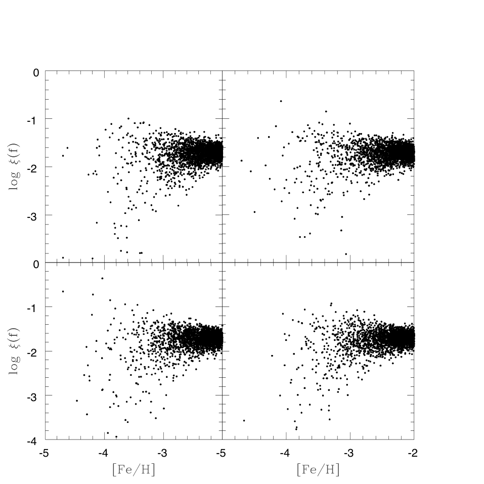
Four realizations of the beta distribution (i.e. no clustering) are presented in Fig. 1; a total of points was used for each simulation distributed in [Fe/H] according to Fig. 2 (see §5). The distribution can be renormalized trivially to match a given set of [Fe/H] vs. [X/Fe] observations (e.g. Fields et al 2002). The beta distribution is everywhere continuous in , and therefore , except in the limit of small or . This recognizes the fact that, as stated by Fields et al (2002), “a given parcel of ISM gas and dust can be enriched to different degrees by the ancestors it had.” But in the limit of small or , discreteness effects may exist. Stars with very few prior enrichments, if they can be identified, provide crucial information on the progenitor yields of class A or B sources (e.g. Shigeyama & Tsujimoto 1998; Karlsson & Gustafsson 2001; Ballero et al 2006), but within the domain of the statistical model, these are rare events and may be difficult to find unambiguously. This is an issue we return to in §5. At high [Fe/H], when new sources of metals become dominant (e.g. type Ia SNe, asymptotic giant branch stars [AGB]), the simple description in equation 3 breaks down.
To recap, the model described by equation 3 assumes that a star with a given [Fe/H] has been enriched to different degrees by its type A and type B ancestors which is considered to be a continuous rather than a discrete process. Equation 3 is used to generate a distribution of possible values of at a constant value of [Fe/H] or equivalently . More complex models show that there is generally no simple relation between and [Fe/H] (e.g. Qian 2001; Bland-Hawthorn & Freeman 2004).
We note already from Fig. 1 that spurious groupings (false positives) are inevitable, particularly when the data points are convolved with typical errors of 0.1 dex psf for differential abundance analysis. The importance of the beta distribution in equation 3 is that it enables us to efficiently generate large numbers of unbiassed realizations () of the theoretical abundance plane, something that is infeasible with full-blown chemical modelling. These are required to calibrate the statistical properties of our group-finding algorithm in §5. This step is necessary if we are to identify significant groups against a rapidly changing background, as observed in Fig. 1. Clusters at low [Fe/H] will have a higher level of significance than abundance groupings at higher [Fe/H] (cf. Karlsson et al 2008) and we need to be able to identify groups with smaller number statistics.
But first we must consider more complex treatments of stochastic chemical evolution that will allow us to include the effects of clustering during star formation.
III.2. Inhomogeneous stochastic model
The chemical evolution model that most resembles our new work is Argast et al (2000, 2004). Their model was computed over a volume (2.5 kpc)3 for a uniform gas mass of 108M⊙ at a resolution of (50 pc)3, such that they were sensitive to chemical inhomogeneities on mass scales as low as 103M⊙. A distinct feature of the Argast model is that star formation mostly occurs in the expanding shell of material swept up by the supernova shock front. They make the simplifying assumption that [X/Fe] is determined by the SN yield such that [Fe/H] is a combination of the SN yield and the swept-up ISM, and that the shell is everywhere fully mixed.
There are several problems with this assumption. First, as far as we are aware, there is no compelling evidence for star formation occurring in supernova remnant shells. The closest one gets are some studies of the Large Magellanic Cloud and the Galaxy (Yamaguchi et al 1999, 2001) which conclude that maybe 10% of star forming regions today appear to be triggered by local supernova events. There is a clear distinction that must be made. If the star formation occurred in collapsing massive clouds triggered by the passing shock wave, rather than in the swept up shell, we would still expect these star clusters to be highly homogeneous.
Secondly, core-collapse supernovae are inherently asymmetric due to the nature of the explosion mechanism due to stellar rotation, magnetic fields, and so on (Wang & Wheeler 2008). Asymmetric ejections from these supernovae are well supported by observations (q.v. Maund et al 2009). Therefore, the remnant shells are highly unlikely to be chemically homogeneous, again supported by x-ray observations of nearby supernova remnants (Wang & Wheeler 2008). Asymmetric enrichment would have led to even larger spread in the elemental abundances, thereby invalidating their model comparisons.
Thirdly, our new homogeneity condition, supported by observation, is essentially independent of the original gas distribution. This constitutes a smoothing scale in mass below which metallicity variations cannot occur, thereby suppressing the amount of scatter observed in the abundance plane (cf. Argast et al 2004).
We now introduce our revised chemical evolution model which incorporates the onset of chemically homogeneous star clusters.
IV. Revised chemical evolution model
IV.1. Initial cluster mass function
In order to derive the impact of star clusters on the abundance plane, we must consider the progenitor mass distribution of star clusters. It is now well established that star clusters have a range of masses that extend from a maximum mass () to a minimum mass (). The form of the birth distribution is known as the initial cluster mass function (ICMF) and is assumed to have the form
| (4) |
The observations may support a universal slope of in all environments, i.e. equal mass per logarithmic bin (Fall, Chandra & Whitmore 2005, 2009; Lada & Lada 2003; Elmegreen 2010). In this picture, the only parameter that does appear to vary at all between galaxies today is , which can be represented schematically as a Schechter function-like cutoff in the ICMF, although there is no good reason to prefer this functional form over a simple truncation.
A power law is logarithmically divergent at both low and high masses, so it must be truncated somewhere. At low masses, the truncation is due to the discreteness of stellar masses – the smallest cluster is simply one star. At large masses, there must also be a truncation. For this reason, and because the molecular cloud mass function (as opposed to the cluster mass function) is observed to have a non-trivial truncation, there is likely to be a maximum cluster mass, and that it varies depending on galactic environment. In disk galaxies, a possible explanation is that the truncation mass is of order the Toomre mass in the galactic disk (Toomre 1964; Escala & Larson 2008), which is M⊙ for the Milky Way, but is significantly larger for present-day starburst/merger galaxies (Larsen 2009) and their high-redshift counterparts (Genzel et al 2006; Forster-Schreiber et al 2009). The situation in spheroidal galaxies is much less clear but the common occurrence of globular clusters indicates that massive cluster formation must take place (Elmegreen 2010).
IV.2. Stochastic chemical evolution
We take as our starting point the stochastic chemical enrichment model presented in Karlsson (2005, 2006) and Karlsson et al. (2008). This model is now updated to include the homogenizing processes that must occur during the formation of star clusters (§2). But in order to do this, two additional mixing processes must be accounted for. First, since stars within clusters show no evidence of scatter in chemical abundance ratios, the gas involved in the formation of a cluster must be homogenized prior to, and stay homogenized during, the formation of the individual stars. We include a mixing process to ensure that this is always true during the cloud collapse and cluster formation phase. Second, since massive stars are short lived ( Myr) they will explode as supernovae (SNe) before the cluster has dispersed. Assuming that the cluster is unbound and that the intrinsic velocity dispersion of the stars in the cluster is km s-1, massive stars will, on average, be pc apart when they go off as SNe. This is less than the typical size ( pc) of a SN remnant (SNR) as it merges with the ambient medium. (e.g. Ryan et al. 1996). Therefore, we assume that the ejecta of all SNe formed within a single cluster enrich the ISM collectively with a mixing mass that scales linearly with the total energy output of the clustered SNe. These two processes, which produce additional averaging of newly synthesized material before a new generation of stars is formed, have not been considered in earlier models.
The mixing volume, , of each chemical enrichment event is given as a power-law expression. The present model is somewhat simplified as we suppress the continuous mixing due to the bulk random motions in the turbulent ISM. Without the time-dependent turbulent diffusion term (cf. Karlsson et al. 2008, equation 1), reduces to
| (5) |
where
| (6) |
is the density of the ISM and is the dilution mass of the ejecta of a number () of SNe as they merge with the ambient medium (e.g. Cioffi, McKee & Bertschinger 1988). Here, we assume that the total dilution mass for the ejecta of multiple SNe exploding in a cluster is proportional, on average, to the total energy released by the SNe associated with that cluster, such that
| (7) |
where is the mass swept-up by individual SNe assuming it explodes in isolation. In order to introduce a small amount of randomness, is drawn from a normal distribution centred on with a width of . Note that this mixing process is denoted a single enrichment event, even though it may involve enrichment by multiple SNe.
In addition to this mixing, there is also a mixing volume associated with the formation of the cluster during the collapse of the molecular cloud, , such that
| (8) |
where is the mass of the molecular cloud associated with the star cluster. Within this volume, everything is assumed to be thoroughly mixed before stars are allowed to form.
In our models, we explore the range (e.g. Kroupa & Boily 2002), between clusters of mass ), which is our fiducial mass range (Larsen 2009; Portegies Zwart et al 2010). We adopt a simple scaling relation between the cluster mass and the mass of the parent molecular cloud, such that , where we adopt a star formation efficiency of (see §2). Similarly, the stellar initial mass function (IMF) is governed by
| (9) |
For simplicity, , which recovers the Salpeter IMF. The range of stellar masses is set to and .
Formally, the average number of clusters contributing to the chemical enrichment in a random point in space can be expressed by the parameter , here given by
| (10) |
where is the fraction of clusters in which SNe explode, while is the formation rate of star clusters, closely related to the star formation rate and . The value of is set by the IMF and the upper mass limit of star clusters. On average, massive stars explode as SNe in a cluster of mass . Such a cluster will not form more than SNe at the -level. We set to be on the safe side.
Now, if we make the simplifying assumtion that star clusters are randomly distributed in space (i.e., not themselves clustered), the probability of finding a region in space enriched by events, i.e., clusters producing one or more SNe, at time is given by the Poisson distribution
| (11) |
To follow the chemical enrichment in a typical dwarf galaxy, we assume a simulation box of kpc on a side, with an initial, constant particle density of cm-3, corresponding to a gas density of g cm-3. The initial mass of baryons in the box is thus which is sufficient to make the largest star clusters considered in this work. The initial metallicity is set to . In the box, star clusters are allowed to form from collapsing molecular clouds. The molecular clouds are distributed randomly within the box and the masses of the corresponding clusters are distributed according to equation (4). During the collapse of a molecular cloud, the volume, , of gas corresponding to the mass of the cloud is made chemically homogeneous. The stars of the cluster will all have chemical abundances equal to those of the parent cloud. The number of massive stars, , in the cluster that will explode as SNe is, again, determined by the Poisson statistics , where the mean number of SNe in a cluster of a given mass is given by
| (12) |
where is the star formation efficiency, is the mass of the molecular cloud, is the fraction of massive stars exploding as SNe, and is the mean stellar mass in a single stellar population. The last two parameters are determined by the IMF. For large values of , the Poisson distribution approaches a normal distribution. We make use of this fact to simplify the calculations for . In clusters where one or more SNe are formed, the ejecta of all SNe, with masses distributed according to equation 9, are homogeneously mixed with the metals already present within the volume . The Fe-core collapse SN yields, in particular of Ca and Fe, are taken from Nomoto et al. (2006) while the yields of Eu, representing r-process elements and assumed to be formed in O-Ne-Mg core collapse SNe in the mass range , are taken from Argast et al. (2004). In order to match the simulations with observations of metal-poor stars in the Galactic halo, the yields of Eu are doubled.
In order to account for the amount of mass locked up in low-mass stars and stellar remnants and the mass lost due to star formation driven galactic outflows, a fraction, , of the mass of each star-forming molecular cloud is subtracted from the total mass of the system. The gas density is decreased accordingly. Infall and mass lost via interaction with the surroundings, such as tidal and ram-pressure stripping are not considered here. When the total mass and gas density of the system has been re-calculated, the next cycle begins with the formation of a new cluster. Since our focus is in the metal-poor regime, the yields of type Ia SNe and AGB stars are not considered here.
IV.3. Results
The results of the clustered simulations for [Ca/Fe] and [r/Fe] with respect to [Fe/H] are presented in Figs. 3 and 4 respectively. For all models, the number of simulated stars is equivalent to a stellar mass of M⊙ and a luminosity of L⊙ assuming a Salpeter IMF; the luminosity is two times higher for a Kroupa IMF. To begin with, we do not consider the effect of distance on the observed number counts; this is treated in §5.2. The modelled number of stars is much larger than we can expect to obtain in nearby dwarfs, but the results provide sufficient resolution to understand the impact of the ICMF parameters. The overall distribution of the stars with metallicity is shown in Fig. 2.
There is a clear progression moving from high to low in the occurrence of clustered abundance signatures. The high limit is indistinguishable from the beta (non-clustered) models. This is not unexpected since, in the limit of , almost all stars are formed in small star clusters such that unique groupings in abundance space are poorly represented.
As decreases, the clustering increases markedly but at the expense of the dispersion in [X/Fe]. In the limit of , the vertical spread has vanished over all [Fe/H] with little or no abundance spread in [X/Fe]. While is smaller than what is observed, it is in fact a useful surrogate for demonstrating the impact of a higher maximum cloud mass for larger values. For example, in Fig. 5, we show the result of running and models with . We see how the high mass cut-off at high mimics the behaviour of a lower value of : the vertical scatter is greatly reduced, and groupings are seen to extend to lower [Fe/H].
In Fig. 6, we show the cumulative fraction of stars and the integrated light as a function of stellar absolute magnitude for the model dwarf galaxy. In Table 1, we give a rough breakdown of how many stars are expected for the dwarf galaxy as a function of stellar apparent magnitude, distance and metallicity. We consider V=16 and V=18 to be the bright and faint limit of an 8m class experiment; these magnitude brackets become V=20 and V=22 on an ELT (Bland-Hawthorn et al 2010).
In the next section, we analyse these simulations using a group finder in order to provide an objective assessment of the amount of measurable clustering in the limit of high and low that we can expect. We apply this analysis for different [Fe/H] cut offs since, as we have seen, the abundance plots become crowded as [Fe/H] increases.
V. Clustering in -space: a statistical treatment
V.1. Group finding for large
In order to investigate the clustering in abundance space (defined by [Fe/H] and [Ca/Fe] or [r/Fe] abundances), we use the density based hierarchical clustering algorithm EnLink [92]. The method is statistically objective and robust in its application; the method is highly efficient and does not use pixellation or binning.
EnLink is based on the fact that a system having more than one group in a data set will have peaks and valleys in the density distribution. A peak in a density distribution identifies a cluster and the set of points which can “climb the peak,” identified by following density gradients, are labeled as its members. The valleys in between the peaks represent intersections between the clusters. These are used to define the boundaries of the clusters and also to form a parent-child relationship, thereby establishing a hierarchical organization of the groups. EnLink works by first calculating the densities of the data points using a set of nearest neighbours and then organizes the points in groups by using nearest neighbour links.
We present our results in the Appendix for both [Ca/Fe] and [r/Fe] for different values of over a wide dynamic range in the observed number of data points. We confirm that statistically significant groupings in abundance space can be recovered, particularly at low values of . For this work, we adopt a low cluster-mass limit of M⊙ which is likely to be too conservative. For a fixed number of simulation particles, decreasing suppresses the number of detected groups.
V.2. Group finding for small
Clustering should be present even in the limit of only a few data points. To emphasize this fact, we have simulated the abundance measurements for a dwarf galaxy at a distance of 30 kpc (see Figs. 8 and 9) as observed on 8m class and 30m class telescopes respectively. We adopt a stellar mass of M⊙ typical of a faint dwarf galaxy. This object has about stars, a luminosity of L⊙ and an absolute V mag of assuming a Salpeter IMF. The luminosity is a factor of two higher for a Kroupa IMF. The star counts are consistent with the model values in Table 1 when scaled to the adopted lower mass.
For the 8m experiment (Fig. 8), we assume measurement errors of 0.1 dex in both [r/Fe] and [Fe/H]. For and , the effects of clustering are evident and this holds true if we double the measurement error. The impact of this measurement uncertainty over the full simulation is shown in Fig. 7. We conclude that, once more extensive studies are made of the nearest dwarf galaxies, the effects of clustering may become evident even before the advent of ELTs. We envisage projects which focus on relatively few stars that appear grouped in abundance space in low resolution spectroscopic data. Long integrations and differential analysis will allow the null hypothesis to be tested that the stars have identical abundances in all elements.
For the 30m experiment (Fig. 9), we have assumed a general improvement in the atmospheric models and the experimental errors, and therefore adopt errors of 0.05 dex. The effects of clustering, which are easily seen, remain clearly visible even after a twofold increase in the measurement errors in both axes. This simulation is a powerful statement of the importance of multi-object echelles on ELTs.
For a fixed and data dimensionality, the number of spurious groups due to Poisson noise increases linearly with the total number of data points . Therefore, EnLink can be used in the limit of small with set to 3, i.e. a minimum of one more than the number of data dimensions. But with so few data points, the full power of EnLink is not being exploited such that more rudimentary statistical techniques may be better. However, EnLink is particularly efficient in treating data sets with more than two dimensions, even in the limit of small .The significance of groups increases dramatically when we apply EnLink on an abundance space with more dimensions. The normalizing distribution in equation 3 is easily extended to higher dimensions. In Fig. 15, we apply EnLink to the 3D -space ([Fe/H], [Ca/Fe], [r/Fe]) for three different measurement errors (0.05, 0.1, 0.2 dex) typical of contemporary observations on 8m telescopes at V=18. Even in the presence of large errors, clustering signals are seen in all cases.
VI. Discussion
This paper has explored the prospect of probing the mass scales of the first star clusters. We stress that we have used a lower cluster-mass limit of M⊙ (typically 10 stars) which is very conservative. A more reasonable value may be an order of magnitude higher (cf. Bland-Hawthorn et al 2010). For and a fixed number of simulation particles, the lower threshold has the effect of reducing cluster membership by a factor of ten, and increasing the “background” by the same factor. This lowers the overall clustering signal by an order of magnitude. But we adopt the conservative lower mass limit in order to account for a possible dwarf stellar population that are not born in clusters. We were unable to find any observational constraints on the diffuse vs. clustered population in dwarf galaxies (cf. Lada & Lada 2003).
In our conservative analysis, we find that there is an intimate connection between properties of the ICMF and the amount of potentially detectable clustering in the abundance plane. A flat ICMF and/or a ICMF with a high mass cut-off produces strong clustering in the [Fe/H] vs. [X/Fe] abundance plane (-space). While our models are inevitably oversimplified, the phenomenon should be detectable on 8-10m telescopes (e.g. Figs. 8 and 9). This gains support from existing observations of open clusters, globular clusters and moving groups (Castro et al 1999; Shen et al 2005; Randich et al 2006; Sestito et al 2007; De Silva, Freeman & Bland-Hawthorn 2009; Chou et al 2010; Bubar & King 2010). A clean “clustering” signature in -space, particularly at low metallicity, is important for a number of reasons. First, it indicates the presence of massive star clusters in the early universe and conceivably provides a constraint on the mass of the first systems. Second, it provides a clean signal of the progenitor abundances in the cloud prior to cluster formation. This abundance measurement is averaged over a substantial amount of gas and is therefore not subject to mixing anomalies (Karlsson & Gustafsson 2001) or mass transfer in binaries (e.g. Suda et al 2004; Ryan et al 2005; Lucatello et al 2005).
Strong clustering would indicate a highly flattened ICMF, or a high mass cut-off. This could herald the onset of the formation of massive star clusters in dwarf galaxies (e.g. Bromm & Clarke 2002). If the star formation efficiencies were low at that time, this may require supermassive gas clouds ( M⊙) to have formed even at the earliest times (Abel et al 2000), possibly consistent with the regular occurrence of massive star-forming clumps at high redshift (Genzel et al 2006; Forster-Schreiber et al 2009; Elmegreen & Elmegreen 2006). Conversely, if such clustering was not observed, then we would infer that the slope of the early ICMF is steep, or the maximum cluster size is relatively small compared to the present day. But the observed scatter would need to be consistent with the non-detection of clustering.
In future investigations, from the perspective of chemical signatures, we will look at the degeneracy between steep ICMFs with a high mass cut-off and flatter ICMFs with a lower mass cut-off (see §4.2). We will also look at a wider class of chemical elements that are considered in numerical simulations of the first stars. We will look at the improvement in cluster identification with more chemical elements, particularly in the limit of small . The clustered abundance signatures will provide unique insight into the most ancient star clusters. These signatures are signposts of the chemistry immediately before the onset of star formation, untainted by mass transfer in close binary pairs or incomplete mixing anomalies.
Finally, it is an extraordinary fact that we can probe back to the first billion years from observations of the local universe. We can say with absolute certainty that stars existed at this time. These were responsible for the first chemical elements (Ryan-Weber, Pettini & Madau 2006) and for reionizing the fog of hydrogen that permeated the early Universe (Fan et al 2002). Precisely when the first star clusters formed is unknown. It seems likely, however, that gas was able to fragment at very high density even at primordial abundance levels (Clark et al 2008). It may be possible to directly probe these environments in an era of the Atacama Large Millimetre Array and the James Webb Space Telescope. But we believe that some of the most important insights, particularly with regard to progenitor yields, will undoubtedly come from near-field cosmology. To this end, it will be necessary to equip the next generation of ELTs with wide-field multi-object spectrographs that operate at high spectroscopic resolution (R20,000).
| Salpeter | Kroupa | |||||||||
|---|---|---|---|---|---|---|---|---|---|---|
| Fe/H | -5:-4 | -4:-3 | -3:-2 | -2:-1 | -5:-4 | -4:-3 | -3:-2 | -2:-1 | ||
| V = 16 | ||||||||||
| 10 | 0.7 | 1.9 | 3.0 | 3.5 | 1.0 | 2.2 | 3.3 | 3.8 | ||
| 30 | - | 0.8 | 1.9 | 2.4 | - | 1.1 | 2.2 | 2.7 | ||
| 100 | - | - | 0.4 | 1.0 | - | - | 0.7 | 1.3 | ||
| V = 18 | ||||||||||
| 10 | 1.1 | 2.3 | 3.4 | 3.9 | 1.4 | 2.6 | 3.7 | 4.2 | ||
| 30 | 0.7 | 1.9 | 3.0 | 3.5 | 0.9 | 2.2 | 3.2 | 3.8 | ||
| 100 | - | 0.6 | 1.7 | 2.2 | - | 0.9 | 2.0 | 2.5 | ||
| V = 20 | ||||||||||
| 10 | 2.2 | 3.4 | 4.5 | 5.0 | 2.5 | 3.7 | 4.8 | 5.3 | ||
| 30 | 1.0 | 2.2 | 3.3 | 3.8 | 1.3 | 2.5 | 3.6 | 4.1 | ||
| 100 | 0.1 | 1.3 | 2.4 | 2.9 | 0.4 | 1.6 | 2.7 | 3.2 | ||
| V = 22 | ||||||||||
| 10 | 2.8 | 4.0 | 5.1 | 5.6 | 3.0 | 4.3 | 5.3 | 5.8 | ||
| 30 | 2.0 | 3.3 | 4.3 | 4.8 | 2.3 | 3.5 | 4.6 | 5.1 | ||
| 100 | 0.9 | 2.1 | 3.2 | 3.7 | 1.2 | 2.4 | 3.4 | 4.0 | ||
References
- [1] Abel, T., Bryan, G. L., & Norman, M. L. 2000, ApJ, 540, 39
- [2] Abel, T., Bryan, G. L., & Norman, M. L. 2002, Science, 295, 93
- [3] André, P., Belloche, A., Motte, F., & Peretto, N. 2007, A&A, 472, 519
- [4] Argast, D., Samland, M., Gerhard, O. E., & Thielemann, F.-K. 2000, A&A, 356, 873
- [5] Argast, D., Samland, M., Thielemann, F.-K., & Qian, Y.-Z. 2004, A&A, 416, 997
- [6] Ascasibar, Y., & Binney, J. 2005, MNRAS, 356, 872
- [7] Audouze, J., & Silk, J. 1995, ApJ, 451, L49
- [8] Ballero, S. K., Matteucci, F., & Chiappini, C. 2006, New Astronomy, 11, 306
- [9] Beers, T. C., & Christlieb, N. 2005, ARA&A, 43, 531
- [10] Belokurov, V., et al. 2009, MNRAS, 397, 1748
- [11] Bland-Hawthorn, J., & Freeman, K. C. 2004, Publications of the Astronomical Society of Australia, 21, 110
- [12] Bland-Hawthorn, J., & Peebles, P. J. E. 2006, Science, 313, 311
- [13] Bland-Hawthorn, J., Krumholz, M., & Freeman, K. 2010, ApJ, 713, 166
- [14] Bromm, V., & Clarke, C. J. 2002, ApJ, 566, L1
- [15] Bromm, V., Coppi, P. S., & Larson, R. B. 2002, ApJ, 564, 23
- [16] Brook, C. B., Kawata, D., Scannapieco, E., Martel, H., & Gibson, B. K. 2007, ApJ, 661, 10
- [17] Bubar, E. J., & King, J. R. 2010, AJ, 140, 293
- [18] Castro, S., Porto de Mello, G. F., & da Silva, L. 1999, MNRAS, 305, 693
- [19] Cayrel, R., et al. 2004, A&A, 416, 1117
- [20] Chou, M.-Y., et al. 2010, ApJ, 708, 1290
- [21] Christlieb, N., et al. 2002, Nature, 419, 904
- [22] Cioffi, D. F., McKee, C. F., & Bertschinger, E. 1988, ApJ, 334, 252
- [23] Clark, P. C., Glover, S. C. O., & Klessen, R. S. 2008, ApJ, 672, 757
- [24] Clark, P. C., Glover, S. C. O., Bonnell, I. A., & Klessen, R. S. 2009, ApJ, submitted, arXiv:0904.3302
- [25] Cohen, J. G., McWilliam, A., Christlieb, N., Shectman, S., Thompson, I., Melendez, J., Wisotzki, L., & Reimers, D. 2007, ApJ, 659, L161
- [26] Coleman, M., Da Costa, G. S., Bland-Hawthorn, J., Martínez-Delgado, D., Freeman, K. C., & Malin, D. 2004, AJ, 127, 832
- [27] De Silva, G. M., Sneden, C., Paulson, D. B., Asplund, M., Bland-Hawthorn, J., Bessell, M. S., & Freeman, K. C. 2006, AJ, 131, 455
- [28] De Silva, G. M., Freeman, K. C., Bland-Hawthorn, J., Asplund, M., & Bessell, M. S. 2007, AJ, 133, 694
- [29] De Silva, G. M., Freeman, K. C., Asplund, M., Bland-Hawthorn, J., Bessell, M. S., & Collet, R. 2007, AJ, 133, 1161
- [30] De Silva, G. M., Freeman, K. C., & Bland-Hawthorn, J. 2009, PASA, 26, 11
- [31] Elmegreen, B. G., & Elmegreen, D. M. 2006, ApJ, 650, 644
- [32] Elmegreen, B. G. 2010, arXiv:1003.0798
- [33] Escala, A., & Larson, R. B. 2008, ApJ, 685, L31
- [34] Fall, S. M., Chandar, R., & Whitmore, B. C. 2005, ApJ, 631, L133
- [35] Fall, S. M., Chandar, R., & Whitmore, B. C. 2009, ApJ, 704, 453
- [36] Fall, S. M., Krumholz, M. R., & Matzner, C. D. 2010, ApJ, 710, L142
- [37] Fan, X., Narayanan, V. K., Strauss, M. A., White, R. L., Becker, R. H., Pentericci, L., & Rix, H.-W. 2002, AJ, 123, 1247
- [38] Feltzing, S., Eriksson, K., Kleyna, J., & Wilkinson, M. I. 2009, A&A, 508, L1
- [39] Fields, B. D., Truran, J. W., & Cowan, J. J. 2002, ApJ, 575, 845
- [40] Förster Schreiber, N. M., et al. 2009, ApJ, 706, 1364
- [41] Frebel, A., et al. 2005, Nature, 434, 871
- [42] Frebel, A., Collet, R., Eriksson, K., Christlieb, N., & Aoki, W. 2008, ApJ, 684, 588
- [43] Frebel, A., Simon, J. D., Geha, M., & Willman, B. 2010, ApJ, 708, 560
- [44] Frebel, A., Kirby, E. N., & Simon, J. D. 2010, Nature, 464, 72
- [45] Freeman, K. & Bland-Hawthorn, J. 2002, ARA&A, 40, 487
- [46] Frinchaboy, P. M., Marino, A. F., Villanova, S., Carraro, G., Majewski, S. R., & Geisler, D. 2008, MNRAS, 391, 39
- [47] Fulbright, J. P., Rich, R. M., & Castro, S. 2004, ApJ, 612, 447
- [48] Genzel, R., et al. 2006, Nature, 442, 786
- [49] Gratton, R., Sneden, C. & Carretta, E. 2004, ARA&A, 42, 385
- [50] Helmi, A. 2008, A&A Rev., 15, 145
- [51] Hennebelle, P., & Chabrier, G. 2008, ApJ, 684, 395
- [52] Heyer, M. H., & Brunt, C. M. 2004, ApJ, 615, L45
- [53] Ibata, R. A., Gilmore, G., & Irwin, M. J. 1995, MNRAS, 277, 781
- [54] Ishimaru, Y., & Wanajo, S. 1999, ApJ, 511, L33
- [55] Izotov, Y. I., & Thuan, T. X. 2004, ApJ, 616, 768
- [56] Joggerst, C. C., Almgren, A., Bell, J., Heger, A., Whalen, D., & Woosley, S. E. 2010, ApJ, 709, 11
- [57] Karlsson, T. 2005, A&A, 439, 93
- [58] Karlsson, T. 2006, ApJ, 641, L41
- [59] Karlsson, T., & Gustafsson, B. 2001, A&A, 379, 461
- [60] Karlsson, T., & Gustafsson, B. 2005, A&A, 436, 879
- [61] Karlsson, T., Johnson, J. L., & Bromm, V. 2008, ApJ, 679, 6
- [62] Kirby, E. N., Simon, J. D., Geha, M., Guhathakurta, P., & Frebel, A. 2008, ApJ, 685, L43
- [63] Koch, A., McWilliam, A., Grebel, E. K., Zucker, D. B., & Belokurov, V. 2008, ApJ, 688, L13
- [64] Kroupa, P., & Boily, C. M. 2002, MNRAS, 336, 1188
- [65] Krumholz, M. R., McKee, C. F., & Klein, R. I. 2005, Nature, 438, 332
- [66] Lada, C. J., & Lada, E. A. 2003, ARA&A, 41, 57
- [67] Larsen, S. S. 2009, A&A, 503, 467
- [68] Lucatello, S., Tsangarides, S., Beers, T. C., Carretta, E., Gratton, R. G., & Ryan, S. G. 2005, ApJ, 625, 825
- [69] Maraston, C., Bastian, N., Saglia, R. P., Kissler-Patig, M., Schweizer, F., & Goudfrooij, P. 2004, A&A, 416, 467
- [70] Mateo, M. L. 1998, ARA&A, 36, 435
- [71] Maund, J. R., Wheeler, J. C., Baade, D., Patat, F., Höflich, P., Wang, L., & Clocchiatti, A. 2009, ApJ, 705, 1139
- [72] McKee, C. F., & Ostriker, E. C. 2007, ARA&A, 45, 565
- [73] McWilliam, A., Simon, J. D., & Frebel, A. 2009, astro2010: The Astronomy and Astrophysics Decadal Survey, 2010, 200
- [74] McWilliam, A. 1997, ARA&A, 35, 503
- [75] Murray, S. D., & Lin, D. N. C. 1990, ApJ, 363, 50
- [76] Nomoto, K., Tominaga, N., Umeda, H., Maeda, K., Ohkubo, T., Deng, J., & Mazzali, P. A. 2005, The Fate of the Most Massive Stars, 332, 374
- [77] Nomoto, K., Tominaga, N., Umeda, H., Kobayashi, C., & Maeda, K. 2006, Nuclear Physics A, 777, 424
- [78] Okrochkov, M., & Tumlinson, J. 2010, ApJ, 716, L41
- [79] Padoan, P., & Nordlund, Å. 2002, ApJ, 576, 870
- [80] Portegies Zwart, S., McMillan, S., & Gieles, M. 2010, arXiv:1002.1961
- [81] Qian, Y.-Z. 2000, ApJ, 534, L67
- [82] Qian, Y.-Z. 2001, ApJ, 552, L117
- [83] Raiteri, C. M., Villata, M., Gallino, R., Busso, M., & Cravanzola, A. 1999, ApJ, 518, L91
- [84] Randich, S., Sestito, P., Primas, F., Pallavicini, R., & Pasquini, L. 2006, A&A, 450, 557
- [85] Roederer, I. U., Kratz, K.-L., Frebel, A., Christlieb, N., Pfeiffer, B., Cowan, J. J., & Sneden, C. 2009, ApJ, 698, 1963
- [86] Ryan, S. G., Norris, J. E., & Beers, T. C. 1996, ApJ, 471, 254
- [87] Ryan, S. G., Aoki, W., Norris, J. E., & Beers, T. C. 2005, ApJ, 635, 349
- [88] Ryan-Weber, E. V., Pettini, M., & Madau, P. 2006, MNRAS, 371, L78
- [89] Scannapieco, E., Kawata, D., Brook, C. B., Schneider, R., Ferrara, A., & Gibson, B. K. 2006, ApJ, 653, 285
- [90] Schneider, R., & Omukai, K. 2010, MNRAS, 402, 429
- [91] Sestito, P., Randich, S., & Bragaglia, A. 2007, A&A, 465, 185
- [92] Sharma, S. & Johnston, K. V. 2009, ApJ, 703, 1061
- [93] Shen, Z.-X., Jones, B., Lin, D. N. C., Liu, X.-W., & Li, S.-L. 2005, ApJ, 635, 608
- [94] Shigeyama, T., & Tsujimoto, T. 1998, ApJ, 507, L135
- [95] Simon, J. D., & Geha, M. 2007, ApJ, 670, 313
- [96] Suda, T., Aikawa, M., Machida, M. N., Fujimoto, M. Y., & Iben, I., Jr. 2004, ApJ, 611, 476
- [97] Tan, J. C., Krumholz, M. R., & McKee, C. F. 2006, ApJ, 641, L121
- [98] Tolstoy, E., Hill, V., & Tosi, M. 2009, ARA&A, 47, 371
- [99] Toomre, A. 1964, ApJ, 139, 1217
- [100] Travaglio, C., Galli, D., & Burkert, A. 2001, ApJ, 547, 217
- [101] Tsuribe, T., & Omukai, K. 2006, ApJ, 642, L61
- [102] Tsuribe, T., & Omukai, K. 2008, ApJ, 676, L45
- [103] Tumlinson, J, 2010, ApJ, 708, 1398
- [104] Venn, K. A., Irwin, M., Shetrone, M. D., Tout, C. A., Hill, V., & Tolstoy, E. 2004, AJ, 128, 1177
- [105] Villanova, S., Randich, S., Geisler, D., Carraro, G., & Costa, E. 2010, A&A, 509, A102
- [106] Walsh, S. M., Jerjen, H., & Willman, B. 2007, ApJ, 662, L83
- [107] Wang, L., & Wheeler, J. C. 2008, ARA&A, 46, 433
- [108] Wasserburg, G. J., & Qian, Y.-Z. 2000, ApJ, 538, L99
- [109] White, S. D. M., & Springel, V. 2000, The First Stars, 327
- [110] Yamaguchi, R., Saito, H., Mizuno, N., Mine, Y., Mizuno, A., Ogawa, H., & Fukui, Y. 1999, PASJ, 51, 791
- [111] Yamaguchi, R., Mizuno, N., Onishi, T., Mizuno, A., & Fukui, Y. 2001, ApJ, 553, L185


Appendix A Group finding in an abundance space
In the EnLink clustering scheme, each group is characterized by a maximum density and a minimum density , and these are used to define its significance as
| (A1) |
where is the standard deviation associated with the density estimator and is a constant for a given dimensionality and .
For Poisson-sampled data the distribution of density as estimated by the code using the kernel scheme is log-normal and the variance satisfies the relation
| (A2) |
where is the number of neighbours employed for density estimation, the volume of a -dimensional unit hypersphere and the norm of the kernel function [92]. For and , evaluates to 0.4714.
Thus Enlink has two free parameters: (i) the significance threshold of the group , and (ii) the number of nearest neighbours used for density estimation. The variable should be set to less than the minimum desired size of the groups because the density is smoothed over a scale of nearest neighbours such that the significance and hence the probability of detecting groups of size less than is drastically reduced. Additionally, neighbours are used for linking the groups which means groups whose density peaks lie within nearest neighbours of each other cannot be separated. Since we are interested in identifying groups with less than 10 data points, we set ; the case for is discussed in the next section.
Our initial analysis is for data points with [Fe/H] -2.5. This includes a crowded, high-density region of the abundance plane which skews the clustering analysis considerably. However, this may be an important regime if the first chemical elements arise from pair instability supernovae (Karlsson et al 2008). The significance of spurious groups is distributed almost as a Gaussian distribution and hence the significance threshold is used to suppress these groups. An improved version of the empirical formula [92] for the expected number of spurious groups, valid for , is given by
| (A3) |
where is a small correction term and is the number of data points.44 4 Since the distribution in for spurious groups is roughly normal (equation 15), can be loosely interpreted as the statistical z-score for finding a group per unit data point. In Figs. 10 and 11, we plot the significance distribution of identified groups for data sets with different values of and as labelled on the plots.
We set such that the expected number of spurious groups (false positives) with is about 2 in all data sets which we calibrate from the beta models. is set to 1.0, 2.35, 3.5 and 4.35 for data with as 100, 300, 1000 and 3000 respectively. This number is increasing because, for a fixed and data dimensionality, the number of spurious groups due to Poisson noise increases linearly with the total number of data points .
Each panel shows the outcome of five EnLink analyses: the cluster-less beta model (solid black line); the simulated models A1 and B1 having unrealistic abundance errors 0.01 dex shown as solid red and blue curves respectively; the simulated models A5 and B5 having abundance errors 0.05 dex shown as dotted red and blue lines respectively. In each panel, the mean number of identified groups along with its dispersion is also given. The mean and dispersion were calculated using 100 random realizations of each data type. The plotted distributions are also averaged over these 100 random realizations. We also provide a measure of the statistical significance of detecting clusters in a data set as follows. If is the number of groups as predicted by the smooth beta model, the statistical significance of clustering in a model is given by
| (A4) |
The third column shows the value of for each data set.
It can be seen in Fig. 10 and 11 that the expected number of spurious groups for the beta models are nearly independent of the value of , which is a consequence of the adaptive metric scheme. Specifically, EnLink uses the concept of a locally adaptive metric, which is used for calculating densities and nearest neighbours of data points (a refinement over earlier developments by Ascasibar & Binney [2005]) to increase the efficiency of detecting clusters in multi-dimensional spaces. If instead clustering is performed using a Euclidean metric on raw data, the significance distribution of spurious groups due to Poisson noise is found to vary with the distribution of points in the abundance space, e.g., the beta models with different values of .
In the limit of few data points, the locally adaptive metric scheme is equivalent to using a metric which is given by the inverse of the dispersion along each dimension. As a check we also performed the analysis using this simpler scheme and found equivalent results, thereby demonstrating the robustness of our group-finding analysis. For the sake of accuracy, we use the beta models to evaluate the significance of clustering, but strictly speaking this is not required and any Poisson sampled cluster-less data would also suffice. In fact, the empirically derived formula given by Equation (A3) can also be used directly to predict the number of spurious groups.
Next we compare the parameter for the different cases. It can be seen that as and increase, increases also. First we look at cases with unrealistic measurement errors of 0.01 dex. It is clear that the models are nearly undetectable for all values of and closely resemble the beta models. For , a minimum value of is needed for . For lower values of , signatures of clustering are visible with as few as 100 points. Increasing the abundance errors to 0.05 dex significantly affects our ability to detect clusters. When sufficient number of data points are present, the A5 and B5 models perform better for and as compared to . This is because the clusters in these cases are more in number, are spread over a larger area, are less crowded, and hence easier to detect.
Since clustering is most prominent for lower values of [Fe/H], we also investigated data sets with a lower metallicity cut-off, [Fe/H] -3.0. These results are shown in Figs. 12 and 13. The parameter is found to increase in general for all cases, unlike what is seen in the [Fe/H] -2.5 analysis (Figs. 10 and 11). It is striking how much better EnLink performs on these simulations which is to be expected given the broader intrinsic dispersions of [r/Fe] in the models. In light of these results, another way to look at Fig. 4 is the significance of clustering over the abundance plane. In Fig. 14, we show the contours for the four different values of with lower significance regions to high [Fe/H]. Clustered abundance data points near the mean value of [r/Fe] are more likely at low [Fe/H] for low values of . Clustered abundance data points away from the mean are favoured by higher values of .