The Value of Staying Current when Beamforming

Feedback delay results in CSI at the transmitter that is inaccurate, and the resulting mismatch between the true channel and the estimate causes errors in code selection. Note that it is possible to base feedback on long-range prediction of rapidly time-varying correlated fading channels (see [6]) but this approach is outside the scope of our model. In our system model, we assume no forward prediction of CSI.

Jakes [11] models the channel state evolution for time-selective narrowband channels as a Markov chain. The autocorrelation of the transfer function as a function of the time difference $\delta{t}$ is derived as

where $J_{0}(\cdot)$ denotes the zero-order Bessel function of the first kind and $f_{d}$ is the maximum Doppler shift. Note that for small $\delta{t}$, the slope of the autocorrelation $\rho$ is strictly negative. We view $\rho$ as a measure of the persistence of the channel - the larger $\|\rho\|$, the stronger is the correlation between the latest channel measurement and the current channel state.

We model channel state persistence by a simple Markov chain as in [12, 13]. We define the current channel state $\tilde{\mathbf{h}}$ in relation to the previous channel estimation $\mathbf{h}$ as

where $\mathbf{e}$ is the deviation from the estimate. The variables $\mathbf{h}$ and $\mathbf{e}$ are independent and each of their components follows the standard complex Gaussian distribution, $\mathop{\it CN}(0,1)$.

In [9], Annapureddy et al. derive the outage probability for a beamforming system that is subject to feedback delay. They show that in the low $\mathop{\mathsf{SNR}}$ regime, power allocation in the direction of the CSI performs better, while uniform spatial power allocation (USPA) is beneficial in high $\mathop{\mathsf{SNR}}$ scenarios. The minimum outage probability for unconstrained codebook cardinality is

where $\Gamma_{k}\left(x\right)$ is the lower incomplete gamma function.

RVQ codebooks are parameterized by their cardinality $N$ and consist of vectors that are isotropic (uniformly distributed over the sphere). We define the tradeoff factor $\nu=\max_{\mathbf{p}\in\mathcal{C}}\frac{|\langle\mathbf{h},\mathbf{p}\rangle|^{2}}{\|\mathbf{h}\|^{2}}$ as the loss of adaptability in comparison to the perfect mutual-information maximizing code due to the limited size of the RVQ codebook. Complex Gaussian distribution of the channel vector and isotropy of the codebook yields the probability density function that appears in [14]

We now extend (6) with the tradeoff factor and average over the probability density function, resulting in

with

Proof: Given $\nu$, the outage probability is

Then, the overall outage probability for random vector quantization beamforming systems of $N$ random vectors is

$\square$

Fig. 1 plots outage probability as a function of persistence; the RVQ codebook has cardinality 8, the transmission rate is 2 bits/s/Hz, and performance of a $4\times 1$ MISO system is compared to that of a similar $2\times 1$ MISO system. Note that loss of persistence results in curves with equal slopes, indicating a loss in MISO diversity order.

In the opposite direction, Fig. 2 starts with a target outage probability and plots the required size of the RVQ codebook as a function of persistence. Note that outage probabilities of 1% are representative of delay sensitive applications such as voice, whereas probabilities of 10% or higher are representative of best effort data services. We see that codebook size grows exponentially with lower persistence and that the rate of growth depends on the target error probability. We expect to explore the value of adapting the choice of codebook in future work.

The diversity order is defined as

Using the fact that $\Gamma_{k}(x)\approx\frac{x^{k}}{k!}$, we approximate the outage probability in high $\mathop{\mathsf{SNR}}$ regime as

where $\gamma_{0}=\frac{2^{R}-1}{\epsilon/N_{t}}$.

Therefore, the diversity order for RVQ beamforming in the presence of feedback delay ($0\leq\rho<1$) is

When there is no delay, the outage probability for RVQ beamforming is

So, the diversity order for RVQ beamforming with no feedback delay is given by

Hence, the diversity order for RVQ beamforming is

Remark: In a open-loop wireless communication systems with $N_{t}$ transmit antennas and single receive antenna, space-time coding helps to achieve the diversity order of $N_{t}$ by scheduling streams across different transmit antennas. Our analysis is based on non-coded beamforming systems. With perfect feedback, it can achieve the diversity order $N_{t}$ and the diversity deteriorates to 1 as feedback becomes delayed. Note that, in the case of delayed feedback, space-time coding can also helps to obtain full diversity.

In Figure 3 we study the possibility of mitigating the degradation effect by increasing the codebook size. Again, we assume a $4\times 1$ MISO setup and plot the outage probability for different codebook sizes at a fixed channel persistence of $\rho=0.9$. Observe that larger codebooks converge towards the perfect beamforming case, but cannot mitigate the loss in diversity order.

In pure TAS scenarios, the transmitter-side antenna is selected for which the channel gain is maximal, hence

$\gamma_{\textrm{TAS}}$ is the largest member of a set of exponentially distributed channel gain values $h_{i}$ with probability density function

Based on the distribution of $\gamma_{\textrm{TAS}}$, we now derive the outage probability for TAS scenarios.

Proof: We recall from equation (6) that $\left|\lambda+\sqrt{2}z\right|^{2}$ is non-central chi-square distributed. For a given $\gamma_{\textrm{TAS}}$ we can therefore derive equality

where $\beta=\frac{\gamma_{0}}{1-\rho^{2}}$ and $F_{(\textrm{nc}-\mathcal{X}^{2},\;n,\;m)}(\cdot)$ is the cumulative probability function for the non-central chi-square distribution with $n$ degrees of freedom and parameter $m$.

So the overall outage probability is

Using the fact that

where $F_{(\mathcal{X}^{2},2+2k)}(\cdot)$ is the cumulative probability function of chi-square distribution with degree $2+2k$ and the fact that

we can rewrite the outage probability as

$\square$

Fig. 4 plots outage probability for TAS beamforming as a function of persistence. The pattern is similar to that for RVQ codebooks; loss of persistence results in curves with equal slopes, indicating a loss in MISO diversity order

In the presence of feedback delay ($0<\rho<1$), the diversity order for TAS is

Hence, the diversity order is given by

Fig. 5 plots outage probability in a low-persistence channel ($\rho=0.8$) as a function of SNR. As expected, Perfect Beamforming (PBF) is superior to RVQ beamforming and Transmit Antenna Selection (TAS). However the gap between PBF and RVQ will narrow as the size of the codebook increases. When the persistence $\rho<1$, all schemes experience a loss in diversity order.

The outage probability for transmit antenna selection with multiuser diversity in the case of no-delay feedback is given in [15]. We extend the analysis to the case of delayed feedback. During each coherent interval, the scheduler selects the $i^{th}$ transmit antenna and the $k^{th}$ user by

where $\mathbf{h}_{i}^{(k)}=\left(h_{i,1}^{(k)},\cdots,h_{i,N_{r}}^{(k)}\right)$ represents the channel vector between the $i^{th}$ transmit antenna and the $k^{th}$ user. Given Maximal Ratio Combining (MRC) at the $\hat{k}^{th}$ user, the received signal $\mathbf{r}^{(\hat{k})}$ is given by

where $\sum_{j=1}^{N_{r}}\langle\mathbf{h}_{\hat{i},j}^{(\hat{k})},\mathbf{n}_{\hat{i},j}^{(\hat{k})}\rangle$ is the combined noise with zero mean and variance $N_{r}$. The cumulative probability function of $\eta=\|\mathbf{h}_{\hat{i}}^{(\hat{k})}\|^{2}$ is given by

where $Z=N_{u}N_{t}$ and its probability density function is given by

The outage probability in the presence of feedback delay is

where $\tilde{\mathbf{h}}_{\hat{i}}^{(\hat{k})}$ is defined in (2) and $z_{j}=\mathbf{e}^{(\hat{k})}_{\hat{i},j}e^{-i\angle\mathbf{h}_{\hat{i},j}^{(\hat{k})}}$ is zero mean complex Gaussian with unit variance. Note that $\sum_{j=1}^{N_{r}}\left|\sqrt{2\mu|\mathbf{h}_{\hat{i},j}^{(\hat{k})}|^{2}}+\sqrt{2}z_{j}\right|^{2}$ is non-central chi-square distributed with $2N_{r}$ degrees of freedom and parameter $\sqrt{2\mu\eta}$.

Using the distribution in (26) and (27), we write the outage probability for a given $\eta$ as

Then, the overall outage probability for multiuser MIMO transmit antenna selection with MRC at the receiver is

Lemma 1 [16]: Let $m$, $n$, $k$ be positive integers and $m\geq n$, then the following equation holds:

$\square$

Now, we derive the outage probability for the multiuser MIMO systems with transmit antenna selection and MRC at the receiver.

Proof: the proof is provided in appendix which uses the result in Lemma 1.$\square$

The diversity order of multiuser MIMO systems with transmit antenna selection and receive maximal ratio combining can be derived as

Remark: Proposition 2 is a special case of proposition 3 by setting $N_{u}=N_{r}=1$.

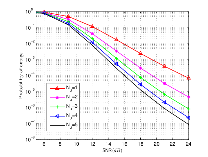
It is shown in Fig. 6 that feedback delay has a great impact on transmit antenna selection in multiuser systems, where it considers 2-user wireless communication system with four transmit antennas at the base station and two receive antenna for each user. Fig. 7 illustrates the outage comparison for systems with different users where their outage probabilities share the same diversity order.

In a $N_{u}$-user system with the base station employing $N_{t}$ transmit antennas and each user equipped with single receive antenna, the base station select the $\hat{k}^{th}$ user via the following algorithm:

Then $\tau=\|\mathbf{h}^{(\hat{k})}\|^{2}$ has the following cumulative density function

and its probability density function is given by

Following the similar calculation for proposition 3, we can derive the outage probability for multiuser MISO systems with perfect beamforming as

Noticing the duality between perfect beamforming for a $M\times 1$ system and maximal ratio combining for a $1\times M$ system, the result in equation (IV-B) can also be easily derived by switching $N_{r}$ and $N_{t}$ in equation (2).

Then, the outage probability for multiuser MISO systems with RVQ beamforming can be easily derived from equation (IV-B) as

where $f_{\nu}$ is defined in equation (9).

The diversity order for multiuser MISO systems with perfect beamforming and RVQ beamforming can be given by

References

- [1] P. Viswanath, D. Tse, and R. Laroia, “Opportunistic beamforming using dumb antennas,” IEEE Transactions on Information Theory, vol. 48, pp. 1277–1294, 2002.
- [2] Y. Wu and R. Calderbank, “Circulant space-time codes for integration with beamforming,” accepted to ICASSP, 2010.
- [3] K. K. Mukkavilli, A. Sabharwal, E. Erkip, and B. Aazhang, “On beamforming with fnite rate feedback in multiple-antenna systems,” IEEE Transactions on Information Theory, vol. 49, pp. 2562–2579, 2003.
- [4] D. J. Love, R. W. Heath, and T. Strohmer, “Grassmannian beamforming for multiple-input multiple-output wireless systems,” IEEE Transactions on Information Theory, vol. 49, pp. 2735–2745, 2003.
- [5] W. Santipach and M. L. Honig, “Capacity of a multi-antenna fading channel with a quantized precoding matrix,” IEEE Transactions on Information Theory, vol. 55, pp. 1218–1234, 2009.
- [6] Y. Wu, T. Jia, A. R. Calderbank, A. Duel-Hallen, and H. Hallen, “Integration of code diversity and long-range channel prediction in wireless communication,” Invited to International Conference on Electromagnetics in Advanced Applications (ICEAA), 2009.
- [7] E. N. Onggosanusi, A. Gatherer, A. G. Dabak, and S. Hosur, “Performance analysis of closed-loop transmit diversity in the presence of feedback delay,” IEEE Transactions on Communications, vol. 49, pp. 1618–1630, 2001.
- [8] K. Huang, B. Mondal, R. W. Heath, and J. G. Andrews, “Effect of feedback delay on multi-antenna limited feedback for temporarily-correlated channels,” Proceedings, IEEE Globecom, 2006.
- [9] V. S. Annapureddy, D. V. Marathe, T. R. Ramya, and S. Bhashyam, “Outage probability of multiple-input and single-output (MISO) systems with delayed feedback,” IEEE Transactions on Communications, vol. 57, pp. 319–326, 2009.
- [10] T. R. Ramya and S. Bhashyam, “Eigen-beamforming with delayed feedback and channel prediction,” ISIT, 2009.
- [11] W. C. Jakes, Microwave Mobile Communication. Wiley, 1974.
- [12] D. Marathe and S. Bhashyam, “Power control for multi-antenna gaussian channels with delayed feedback,” Proceedings of the 39th Asilomar Conference on Signals, Systems and Computers, 2005.
- [13] H. T. Nguyen, J. B. Andersen, and G. F. Pedersen, “Capacity and performance of MIMO systems under the impact of feedback delay,” PIMRC, 2004.
- [14] C. K. Au-Yeung and D. J. Love, “On the performance of random vector quantization limited feedback beamforming in a miso system,” IEEE Transactions on Wireless Communications, vol. 6, pp. 458–462, 2007.
- [15] X. Zhang, F. Chen, and W. Wang, “Outage probability study of multiuser diversity in mimo transmit antenna selection systems,” IEEE Signal Processing Letters, vol. 14, pp. 161–164, 2007.
- [16] D. E. Knuth, The art of computer programming, vol 1: fundamental algorithms. Addison Welsley, Reading, Massachusetts, 1968.