Hořava-Lifshitz Cosmology: A Review

Publication type: Topical Review

Shinji Mukohyama Affiliation: Institute for the Physics and Mathematics of the Universe (IPMU) Affiliation: The University of Tokyo Affiliation: 5-1-5 Kashiwanoha, Kashiwa, Chiba 277-8582, Japan

Abstract

This article reviews basic construction and cosmological implications of a power-counting renormalizable theory of gravitation recently proposed by Hořava. We explain that (i) at low energy this theory does not exactly recover general relativity but instead mimic general relativity plus dark matter; that (ii) higher spatial curvature terms allow bouncing and cyclic universes as regular solutions; and that (iii) the anisotropic scaling with the dynamical critical exponent $z=3$ solves the horizon problem and leads to scale-invariant cosmological perturbations even without inflation. We also comment on issues related to an extra scalar degree of freedom called scalar graviton. In particular, for spherically-symmetric, static, vacuum configurations we prove non-perturbative continuity of the $\lambda\to 1+0$ limit, where $\lambda$ is a parameter in the kinetic action and general relativity has the value $\lambda=1$ . We also derive the condition under which linear instability of the scalar graviton does not show up.

(IPMU10-0120)

1 Introduction

One of the biggest difficulties in attempts toward the theory of quantum gravity is the fact that general relativity is non-renormalizable. This would imply loss of theoretical control and predictability at high energies. In January 2009, Hořava proposed a new theory of gravity to evade this difficulty by invoking a Lifshitz-type anisotropic scaling at high energy [1]. This theory, often called Hořava-Lifshitz gravity, is power-counting renormalizable and is expected to be renormalizable and unitary. Having a new candidate theory for quantum gravity, it is important to investigate its cosmological implications.

There are a number of interesting cosmological implications of Hořava-Lifshitz gravity. For example, higher spatial curvature terms lead to regular bounce solutions in the early universe [2, 3]. Higher curvature terms might also make the flatness problem milder [4]. The anisotropic scaling with $z=3$ solves the horizon problem and leads to scale-invariant cosmological perturbations without inflation [5]. The anisotropic scaling provides a new mechanism for generation of primordial magnetic seed field [6], and also modifies the spectrum of gravitational wave background via a peculiar scaling of radiation energy density [7]. In parity-violating version of the theory, circularly polarized gravitational waves can also be generated in the early universe [8]. The lack of local Hamiltonian constraint leads to dark matter as an integration “constant” [9, 10].

The purpose of this article is to review basic construction of the theory and some of its cosmological implications. In Sec. 2 we explain basics of Hořava-Lifshitz gravity, such as power-counting argument, symmetry, basic quantities, action and equations of motion. In Sec. 3 we comment on issues related to an extra scalar degree of freedom called scalar graviton, and consider the limit in which general relativity is supposed to be recovered. We explicitly see the known result that the naive metric perturbation breaks down in this limit for the scalar graviton. However, this does not necessarily imply the loss of predictability. Indeed, for spherically-symmetric, static, vacuum configurations we shall show that the limit is non-perturbatively continuous. This result might correspond to what is called Vainshtein mechanism [11] in theories of massive gravity [12] and suggest that the extra scalar degree of freedom might safely decouple from the rest of the world in the limit. In Sec. 4 we shall review some of cosmological implications: the dark matter as an integration “constant”, bouncing and cyclic universes and generation of scale-invariant cosmological perturbation without inflation. Finally, Sec. 5 is devoted to a summary of this article and some discussions.

2 Hořava-Lifshitz gravity

2.1 Preliminaries

2.1.1 Power-counting

Let us begin with heuristically explaining the usual power-counting argument in field theory. As the simplest example, let us consider a scalar field with the canonical kinetic term:

\frac{1}{2}\int dtd^{3}\vec{x}\ \dot{\phi}^{2},

(1)

where an overdot represents a time derivative. The scaling dimension of the scalar field $\phi$ is determined by demanding that the kinetic term be invariant under the scaling

t\to bt,\quad\vec{x}\to bx,\quad\phi\to b^{-s}\phi,

(2)

where $b$ is an arbitrary number and $s$ is the scaling dimension to be determined. The invariance of the kinetic term under the scaling leads to the condition

1+3-2-2s=0,

(3)

where $1$ comes from $dt$ , $3$ from $d^{3}\vec{x}$ , $-2$ from two time derivatives and $-2s$ from two $\phi$ ’s. Thus, we obtain $s=1$ . In other words, the scalar field scales like energy. With this scaling in mind, it is easy to see that an $n$ -th order interaction term behaves as

\int dtd^{3}\vec{x}\phi^{n}\propto E^{-(1+3-ns)},

(4)

where $E$ is the energy scale of the system of interest. Here, the minus sign in the exponent comes from $-1$ in $E\to b^{-1}E$ , $1$ in the parentheses comes from $dt$ , $3$ from $d^{3}\vec{x}$ and $-ns$ from $\phi^{n}$ . Now, it is expected that we have a good theoretical control of ultraviolet (UV), i.e. high $E$ , behaviors if the exponent is non-positive. Since $s=1$ , this condition leads to $n\leq 4$ . This is the power-counting renormalizability condition.

We are interested in gravity. Unfortunately, Einstein gravity is not power-counting renormalizable. This is because the curvature is a highly nonlinear functional of the metric and there are graviton interaction terms with $n$ higher than $4$ . The non-renormalizability is one of difficulties in attempts to quantize general relativity.

2.1.2 Abandoning Lorentz symmetry

As already stated, Hořava-Lifshitz gravity is power-counting renormalizable. How does it evade the above argument? The basic idea is very simple but potentially dangerous: abandoning Lorentz symmetry and invoking a different kind of scaling in the UV. The scaling invoked here, often called anisotropic scaling or Lifshitz scaling, is

t\to b^{z}t,\quad\vec{x}\to bx,\quad\phi\to b^{-s}\phi,

(5)

where $z$ is a number called dynamical critical exponent.

Let us now see how the power-counting argument changes if the scaling is anisotropic as in (5). Invariance of the canonical kinetic term (1) under this scaling leads to

z+3-2z-2s=0,

(6)

where $z$ comes from $dt$ , $3$ from $d^{3}\vec{x}$ , $-2z$ from two time derivatives and $-2s$ from two $\phi$ ’s. Then we obtain

s=\frac{3-z}{2}.

(7)

This of course recovers the previous result $s=1$ for $z=1$ . What is interesting here is that $s=0$ if $z=3$ . This implies that, if $z=3$ , the amplitude of quantum fluctuations of $\phi$ does not change as the energy scale of the system changes. The $n$ -th order interaction term behaves as

\int dtd^{3}\vec{x}\phi^{n}\propto E^{-(z+3-ns)/z},

(8)

where $-1/z$ in the exponent comes from $-z$ in $E\to b^{-z}E$ , $z$ in the parentheses comes from $dt$ , $3$ from $d^{3}\vec{x}$ and $-ns$ from $\phi^{n}$ . For $z=3$ (and thus $s=0$ ), the exponent is negative for any $n$ and, therefore, any nonlinear interactions are power-counting renormalizable. For $z>3$ , the theory is power-counting super-renormalizable.

From the above consideration, it is expected that gravity may become renormalizable if the anisotropic scaling with $z\geq 3$ is realized in the UV.

2.1.3 Scalar field action

We would like to realize the anisotropic scaling with $z\geq 3$ in the UV to construct renormalizable nonlinear theories. On the other hand, in order to recover the Lorentz invariance in the infrared (IR), we would like to realize the usual scaling with $z=1$ at low energy. A simple example is a scalar field with the following free-part action:

I_{free}=\frac{1}{2}\int dtd^{3}\vec{x}\left(\dot{\phi}^{2}+\phi{\cal O}\phi\right),

(9)

where

{\cal O}=\frac{\Delta^{3}}{M^{4}}-\frac{\kappa\Delta^{2}}{M^{2}}+c_{\phi}^{2}\Delta-m_{\phi}^{2},

(10)

$M$ is the energy scale corresponding to the transition from the $z=1$ scaling to the $z=3$ scaling, $\kappa$ is a constant, $c_{\phi}$ is the sound speed, i.e. the limit of speed in the IR, $m_{\phi}$ is the mass of the field, and $\Delta$ is the Laplacian in the $3$ -dimensional space ¹¹ 1 If photons have this kind of dispersion relation with $\kappa=O(1)$ , $c_{\phi}=1$ and $m_{\phi}=0$ then experiments such as Fermi GBM/LAT [13] and MAGIC [14] set a lower bound on $M$ as $M>10^{11}GeV$ ..

In the UV, the sixth-order spatial derivative term dominates over lower-order terms and balances with the time kinetic term which includes two time derivatives. This naturally leads to the $z=3$ scaling. On the other hand, in the IR, the second-order spatial derivative term and the mass term are dominant and, thus, the $z=1$ scaling is realized. In this way, it is possible to realize the $z=3$ scaling in the UV and the $z=1$ scaling in the IR.

However, one must be aware that all “constants” in the action are subject to running under the renormalization group (RG) flow. Of course, the sound speed is not an exception. If we consider many fields then the sound speed for each field should run under the RG flow [15]. We need a mechanism or symmetry to make sound speeds of different species to be essentially the same at low energies. More generally speaking, we need a mechanism or symmetry to suppress Lorentz violating operators at low energies. Perhaps, embedding the theory into a larger theory is necessary. One such possibility is related to supersymmetry [16].

2.2 Symmetry

As explained in the previous subsection, the way the power-counting renormalizability is achieved is to violate the Lorentz invariance and to invoke the anisotropic scaling with the dynamical critical exponent $z\geq 3$ . Since the Lorentz invariance is not respected, we treat the time coordinate $t$ and the spatial coordinates $\vec{x}^{i}$ ( $i=1,2,3$ ) separately.

The fundamental symmetry of the theory is the invariance under space-independent time reparametrization and time-dependent spatial diffeomorphism:

t\to t^{\prime}(t),\quad\vec{x}\to\vec{x}^{\prime}(t,\vec{x}).

(11)

The time-dependent spatial diffeomorphism allows an arbitrary change of spatial coordinates on each constant time surface. However, the time reparametrization here is not allowed to depend on spatial coordinates. As a result, unlike general relativity, in Hořava-Lifshitz gravity the foliation of spacetime by constant time hypersurfaces is not just a choice of coordinates but is a physical entity. Indeed, the foliation is preserved by the symmetry transformation (11). For this reason, the map (11) is called foliation preserving diffeomorphism.

In addition to the foliation preserving diffeomorphism invariance, we assume that the theory is invariant under the spatial parity $\vec{x}\to-\vec{x}$ [17] and the time reflection $t\to-t$ .

Finally, in order to render the theory power-counting renormalizable, we would like to realize the anisotropic scaling with $z\geq 3$ at high energy. In the present article, for concreteness, we mainly focus on the case with $z=3$ .

2.3 Basic quantities and projectability condition

Basic quantities of Hořava-Lifshitz gravity are

\mbox{lapse}:N(t),\quad\mbox{shift}:N^{i}(t,\vec{x}),\quad\mbox{$3$d metric}:g_{ij}(t,\vec{x}),

(12)

from which we can construct a four-dimensional spacetime metric of the ADM form as

ds^{2}=-N^{2}dt^{2}+g_{ij}(dx^{i}+N^{i}dt)(dx^{j}+N^{j}dt).

(13)

While the shift $N^{i}$ and the $3$ d metric $g_{ij}$ depend on both the time coordinate $t$ and the spatial coordinates $\vec{x}$ , the lapse $N$ is assumed to be a function of the time only. This condition on the lapse is called the projectability condition.

The projectability condition stems from the foliation preserving diffeomorphism. The lapse represents a gauge freedom associated with the space-independent time reparametrization $t\to t^{\prime}(t)$ and, thus, it is fairly natural to restrict it to be space-independent ²² 2 Abandoning the projectability condition leads to phenomenological obstacles [18] and theoretical inconsistency [19]. On the other hand, the criticisms made in [18, 19] do not apply if the projectability condition is respected.. Of course, the projectability condition is compatible with the foliation preserving diffeomorphism. The transformation of the basic quantities (12) under the infinitesimal foliation preserving diffeomorphism,

\delta t=f(t),\quad\delta\vec{x}^{i}=\xi^{i}(t,\vec{x}),

(14)

is defined as follows.

$\displaystyle\delta N$	$\displaystyle=$	$\displaystyle\partial_{t}(Nf),$
$\displaystyle\delta N^{i}$	$\displaystyle=$	$\displaystyle\partial_{t}(N^{i}f)+\partial_{t}\xi^{i}+{\cal L}_{\xi}N^{i},$
$\displaystyle\delta(N_{i})$	$\displaystyle=$	$\displaystyle\partial_{t}(N_{i}f)+g_{ij}\partial_{t}\xi^{j}+{\cal L}_{\xi}N_{i},$
$\displaystyle\delta g_{ij}$	$\displaystyle=$	$\displaystyle f\partial_{t}g_{ij}+{\cal L}_{\xi}g_{ij},$	(15)

where $N_{i}=g_{ij}N^{j}$ . Note that $\delta N$ is independent of spatial coordinates since $f$ and $N$ are functions of time only. Thus the projectability condition is compatible with the foliation preserving diffeomorphism: the foliation preserving diffeomorphism maps a space-independent $N$ to a space-independent $N$ .

The equation of motion for the lapse corresponds to the generator of the time reparametrization and is called the Hamiltonian constraint. Since the lapse is independent of spatial coordinates, its variations are also space-independent. This means that the Hamiltonian constraint in Hořava-Lifshitz gravity is not a local equation but an equation integrated over a whole space. In subsection 4.1 we shall discuss cosmological implication of the global nature of the Hamiltonian constraint.

2.4 Action

The theory should respect the foliation preserving diffeomorphism. We can then use the following ingredients in the action:

Ndt,\quad\sqrt{g}d^{3}\vec{x},\quad g_{ij},\quad D_{i},\quad R_{ij},

(16)

where $g$ is the determinant of $g_{ij}$ , $D_{i}$ is the $3$ -dimensional covariant derivative compatible with $g_{ij}$ and $R_{ij}$ is the Ricci tensor of $g_{ij}$ . Note that the Ricci tensor includes all information about the Riemann tensor since Weyl tensor identically vanishes in $3$ -dimensions.

2.4.1 The UV action

We should include time-derivative of the $3$ -dimensional metric in the action in order to make the metric dynamical. However, $\dot{g}_{ij}$ is not covariant under the spatial diffeomorphism and, therefore, $\dot{g}_{ij}$ should appear in the action as a part of the covariant quantity called extrinsic curvature,

K_{ij}=\frac{1}{2N}\left(\dot{g}_{ij}-D_{i}N_{j}-D_{j}N_{i}\right).

(17)

The extrinsic curvature transforms as a second-rank symmetric tensor under the spatial diffeomorphism and as a scalar under the time reparametrization. The time kinetic term for the metric is obtained by squaring the extrinsic curvature and properly contracting indices. There are two ways to contract indices:

I_{kin}=\frac{1}{16\pi G}\int Ndt\sqrt{g}d^{3}\vec{x}\left(K^{ij}K_{ij}-\lambda K^{2}\right),

(18)

where $G$ and $\lambda$ are constants, and $K=K^{i}_{i}$ . In general relativity, $\lambda$ is fixed to $1$ because of higher symmetry. On the other hand, in Hořava-Lifshitz gravity, any value of $\lambda$ is compatible with the foliation preserving diffeomorphism invariance and thus $\lambda$ is not fixed. We shall not include terms including derivatives of the extrinsic curvature in the action. This is consistent if the theory without those higher derivative terms is renormalizable: those terms would be non-renormalizable and thus would not be generated by quantum correction. For the same reason, we shall not include terms cubic or higher order in the extrinsic curvature.

Invariant terms made of time derivatives of the shift would inevitably include second or higher time derivatives of the spatial metric. For the reason explained above, we shall not include those higher derivative terms in the action. Time derivative of the lapse corresponds to the connection in $1$ -dimension spanned by the time but the curvature in $1$ -dimension is always zero. Thus, there is no invariant term made of time derivatives of the lapse. Of course, the spatial derivative of the lapse vanishes because of the projectability condition.

Since terms in the kinetic action (18) include two time derivatives, we should include terms with six spatial derivatives in order to realize the $z=3$ scaling in the UV. (For a general choice of $z$ ( $\geq 3$ ) in the UV, we should include terms with $2z$ spatial derivatives.) The foliation preserving diffeomorphism invariance allows five such terms in the action,

	$\displaystyle I_{z=3}$	$\displaystyle=$	$\displaystyle\int Ndt\sqrt{g}d^{3}\vec{x}\left[c_{1}D_{i}R_{jk}D^{i}R^{jk}\right.$		(19)
			$\displaystyle\left.+c_{2}D_{i}RD^{i}R+c_{3}R_{i}^{j}R_{j}^{k}R_{k}^{i}+c_{4}RR_{i}^{j}R_{j}^{i}+c_{5}R^{3}\right],$		(19)

where $c_{i}$ ( $i=1,\cdots,5$ ) are constants. Note that the other possible term $D_{i}R_{jk}D^{j}R^{ki}$ is a linear combination of the above terms up to total derivative and, thus, does not have to be included explicitly. We do not include terms with more than six spatial derivatives since they would be non-renormalizable and thus would not be generated by quantum corrections if the theory without them is renormalizable.

2.4.2 Relevant deformations in the IR

In the IR, terms with less number of spatial derivatives in the action become important. There are two independent terms with four spatial derivatives

I_{z=2}=\int Ndt\sqrt{g}d^{3}\vec{x}\left[c_{6}R_{i}^{j}R_{j}^{i}+c_{7}R^{2}\right],

(20)

one term with two spatial derivatives

I_{z=1}=c_{8}\int Ndt\sqrt{g}d^{3}\vec{x}\ R,

(21)

and a constant

I_{z=0}=c_{9}\int Ndt\sqrt{g}d^{3}\vec{x}\ ,

(22)

where $c_{i}$ ( $i=6,\cdots,9$ ) are constants.

We have written down all possible terms consistent with the symmetry of the theory except for terms involving more than two time derivatives and terms with more than six spatial derivatives. As already stated, those higher-derivative terms excluded in the above construction would be non-renormalizable and, thus, would not be generated by quantum corrections if the theory without them is renormalizable. The theory defined in this way is power-counting renormalizable and, thus, expected to be renormalizable although renormalizability beyond the power-counting argument has not been proved. Also, the theory is expected to be unitary since the action does not include more than two time derivatives. Note that the constants $G$ , $\lambda$ and $c_{i}$ ( $i=1,\cdots,9$ ) are subject to running under the RG flow.

2.4.3 IR action with $z=1$

In the UV the theory naturally exhibits the $z=3$ scaling as the second time derivative terms $I_{kin}$ and the sixth spatial derivative terms $I_{z=3}$ balance with each other.

On the other hand, in the IR the forth and sixth spatial derivative terms, $I_{z=2}$ and $I_{z=3}$ , are unimportant. We therefore have the following action describing the IR behavior of the theory:

	$\displaystyle I_{IR}$	$\displaystyle=$	$\displaystyle I_{kin}+I_{z=1}+I_{z=0}$		(23)
		$\displaystyle=$	$\displaystyle\frac{M_{Pl}^{2}}{2}\int Ndt\sqrt{g}d^{3}\vec{x}\left(K^{ij}K_{ij}-\lambda K^{2}+R-2\Lambda\right),$		(23)

where $M_{Pl}^{2}\equiv 1/(8\pi G)$ and $\Lambda\equiv-8\pi Gc_{9}$ , and we have set $16\pi Gc_{8}$ to unity by rescaling of the time coordinate. This IR action naturally exhibits the $z=1$ scaling. Moreover, the action looks identical to the Einstein-Hilbert action in the ADM formalism if $\lambda\to 1$ . There are however two important differences: (i) $\lambda$ does not have to be $1$ and is subject to running under the RG flow; (ii) the projectability condition restricts the lapse $N$ to be a function of the time only. Regarding (i), the RG flow of the theory has not been investigated and, thus, we do not know whether $\lambda=1$ is an IR fixed point of the RG flow or not. On the other hand, we shall discuss cosmological implication of the point (ii) in subsection 4.1.

2.5 Equations of motion

Adding the matter action $I_{m}$ , the total action is

$\displaystyle I$	$\displaystyle=$	$\displaystyle I_{g}+I_{m},$	(24)
$\displaystyle I_{g}$	$\displaystyle=$	$\displaystyle\frac{M_{Pl}^{2}}{2}\int Ndt\sqrt{g}d^{3}\vec{x}(K^{ij}K_{ij}-\lambda K^{2}+\Lambda+R+L_{z>1}),$	(25)
$\displaystyle\frac{M_{Pl}^{2}}{2}L_{z>1}$	$\displaystyle=$	$\displaystyle(c_{1}D_{i}R_{jk}D^{i}R^{jk}+c_{2}D_{i}RD^{i}R+c_{3}R_{i}^{j}R_{j}^{k}R_{k}^{i}$	(26)
		$\displaystyle+c_{4}RR_{i}^{j}R_{j}^{i}+c_{5}R^{3})+(c_{6}R_{i}^{j}R_{j}^{i}+c_{7}R^{2}).$	(26)

Here, we have rescaled the time coordinate to set $16\pi Gc_{8}$ to unity. Note that not only the gravitational action $I_{g}$ but also the matter action $I_{m}$ should be invariant under the foliation-preserving diffeomorphism.

By variation of the action with respect to the lapse $N(t)$ , we obtain the Hamiltonian constraint

H_{g\perp}+H_{m\perp}=0,

(27)

where

H_{g\perp}\equiv-\frac{\delta I_{g}}{\delta N}=\int d^{3}\vec{x}{\cal H}_{g\perp},\ H_{m\perp}\equiv-\frac{\delta I_{m}}{\delta N},

(28)

and

{\cal H}_{g\perp}=\frac{M_{Pl}^{2}}{2}\sqrt{g}(K^{ij}p_{ij}-\Lambda-R-L_{z>1}),\quad p_{ij}\equiv K_{ij}-\lambda Kg_{ij}.

(29)

Variation with respect to the shift $N^{i}(t,x)$ leads to the momentum constraint

{\cal H}_{gi}+{\cal H}_{mi}=0,

(30)

where

{\cal H}_{gi}\equiv-\frac{\delta I_{g}}{\delta N^{i}}=-M_{Pl}^{2}\sqrt{g}D^{j}p_{ij},\quad{\cal H}_{mi}\equiv-\frac{\delta I_{m}}{\delta N^{i}}.

(31)

Note that the gravitational part of the momentum constraint is determined solely by the kinetic terms and thus is totally insensitive to the structure of higher spatial curvature terms. In particular, for $\lambda=1$ the momentum constraint agrees with that in general relativity.

For comparison, let us consider the case in which the matter sector recovers spacetime diffeomorphism invariance. In this case it makes sense to define the stress-energy tensor $T_{\mu\nu}$ of matter and then

H_{m\perp}=\int d^{3}\vec{x}\sqrt{g}\ T_{\mu\nu}n^{\mu}n^{\nu},\quad{\cal H}_{mi}=\frac{1}{\sqrt{g}}T_{i\mu}n^{\mu},

(32)

where

n_{\mu}dx^{\mu}=-Ndt,\quad n^{\mu}\partial_{\mu}=\frac{1}{N}(\partial_{t}-N^{i}\partial_{i}).

(33)

As in general relativity, the gravitational action can be written as the sum of kinetic terms and constraints up to boundary terms:

I_{g}=\int dtd^{3}\vec{x}\left[\pi^{ij}\partial_{t}g_{ij}-N^{i}{\cal H}_{gi}\right]-\int dtNH_{g\perp}+(\mbox{boundary terms}),

(34)

where $\pi^{ij}$ is momentum conjugate to $g_{ij}$ given by

\pi^{ij}\equiv\frac{\delta I_{g}}{\delta(\partial_{t}g_{ij})}=M_{Pl}^{2}\sqrt{g}p^{ij},\quad p^{ij}\equiv g^{ik}g^{jl}p_{kl}.

(35)

The Hamiltonian corresponding to the time $t$ is the sum of constraints and boundary terms as

H_{g}[\partial_{t}]=NH_{g\perp}+\int d^{3}\vec{x}N^{i}{\cal H}_{gi}+(\mbox{boundary terms}).

(36)

Finally, by variation with respect to $g_{ij}(t,x)$ , we obtain the dynamical equation

{\cal E}_{gij}+{\cal E}_{mij}=0,

(37)

where

{\cal E}_{gij}\equiv g_{ik}g_{jl}\frac{2}{N\sqrt{g}}\frac{\delta I_{g}}{\delta g_{kl}},\quad{\cal E}_{mij}\equiv g_{ik}g_{jl}\frac{2}{N\sqrt{g}}\frac{\delta I_{m}}{\delta g_{kl}}=T_{ij}.

(38)

Note that the matter sector (as well as the gravity sector) should be invariant under spatial diffeomorphism (as a part of the foliation preserving diffeomorphism) and thus it makes sense to define $T_{ij}$ in general. The explicit expression for ${\cal E}_{gij}$ is given by

	$\displaystyle{\cal E}_{gij}$	$\displaystyle=$	$\displaystyle M_{Pl}^{2}\left[-\frac{1}{N}(\partial_{t}-N^{k}D_{k})p_{ij}+\frac{1}{N}(p_{ik}D_{j}N^{k}+p_{jk}D_{i}N^{k})\right.$		(39)
			$\displaystyle\left.-Kp_{ij}+2K_{i}^{k}p_{kj}+\frac{1}{2}g_{ij}K^{kl}p_{kl}+\frac{1}{2}\Lambda g_{ij}-G_{ij}\right]+{\cal E}_{z>1ij},$		(39)

where ${\cal E}_{z>1ij}$ is the contribution from $L_{z>1}$ and $G_{ij}$ is Einstein tensor of $g_{ij}$ .

The invariance of $I_{\alpha}$ under the infinitesimal transformation (15) leads to the following conservation equations, where $\alpha$ represents $g$ or $m$ .

	$\displaystyle 0$	$\displaystyle=$	$\displaystyle N\partial_{t}H_{\alpha\perp}+\int d^{3}\vec{x}\left[N^{i}\partial_{t}{\cal H}_{\alpha i}+\frac{1}{2}N\sqrt{g}{\cal E}_{\alpha}^{ij}\partial_{t}g_{ij}\right],$		(40)
	$\displaystyle 0$	$\displaystyle=$	$\displaystyle\frac{1}{N}(\partial_{t}-N^{j}D_{j})\left(\frac{{\cal H}_{\alpha i}}{\sqrt{g}}\right)+K\frac{{\cal H}_{\alpha i}}{\sqrt{g}}-\frac{1}{N}\frac{{\cal H}_{\alpha i}}{\sqrt{g}}D_{i}N^{j}-D^{j}{\cal E}_{\alpha ij}.$		(41)

3 Scalar graviton and the $\lambda\to 1+0$ limit

3.1 Propagating degrees of freedom

In order to identify propagating degrees of freedom, let us consider linear perturbations around a flat background without matter. We can decompose the perturbation into scalar, vector and tensor parts, according to the transformation under infinitesimal spatial diffeomorphism. Thus, we have

	$\displaystyle N$	$\displaystyle=$	$\displaystyle 1+A,\quad N_{i}=\partial_{i}B+n_{i},$
	$\displaystyle g_{ij}$	$\displaystyle=$	$\displaystyle(1+2\zeta)\delta_{ij}+2\partial_{i}\partial_{j}h_{L}+\partial_{i}h_{j}+\partial_{j}h_{i}+h_{ij},$		(42)

where $n_{i}$ and $h_{i}$ are transverse and $h_{ij}$ is transverse traceless: $\delta^{ij}\partial_{i}n_{j}=\delta^{ij}\partial_{i}h_{j}=0$ , $\delta^{ij}\partial_{i}h_{jk}=0$ and $\delta^{ij}h_{ij}=0$ . Also, $A$ depends only on $t$ because of the projectability condition. By fixing the gauge degrees of freedom $f(t)$ and $\xi_{i}(t,\vec{x})$ as $f=-\int Adt$ and $\xi_{i}=-\partial_{i}h_{L}-h_{i}$ , the gauge transformation (15) leads to

N=1,\quad N_{i}=\partial_{i}B+n_{i},\quad g_{ij}=(1+2\zeta)\delta_{ij}+h_{ij}.

(43)

In this gauge, the momentum constraint (30) without matter is

\partial_{i}\left[(3\lambda-1)\dot{\zeta}-(\lambda-1)\partial^{2}B\right]+\frac{1}{2}\partial^{2}n_{i}=0,

(44)

leading to

B=\frac{3\lambda-1}{\lambda-1}\frac{\dot{\zeta}}{\partial^{2}},\quad n_{i}=0,

(45)

where $\partial^{2}\equiv\delta^{ij}\partial_{i}\partial_{j}$ is the spatial Laplacian. We do not have to solve the Hamiltonian constraint since it is an equation integrated over a whole space and thus does not reduce the number of local physical degrees of freedom. The scalar physical degree of freedom $\zeta$ is often called scalar graviton while the tensor perturbation $h_{ij}$ represents the two physical degrees of freedom of usual tensor graviton.

The time kinetic term expanded up to quadratic order is

I_{kin}=M_{Pl}^{2}\int dtd^{3}\vec{x}\left[\frac{3\lambda-1}{\lambda-1}\dot{\zeta}^{2}+\frac{1}{8}\delta^{ik}\delta^{jl}\dot{h}_{ij}\dot{h}_{kl}\right]+O(\epsilon^{3}),

(46)

where we have introduced a small expansion parameter $\epsilon$ and considered $\zeta$ and $h_{ij}$ as $O(\epsilon)$ . In order to avoid ghost instability, thus $\lambda$ must be either larger than $1$ or smaller than $1/3$ [1]. Since general relativity has $\lambda=1$ and we would like to recover something similar to general relativity in the IR, we should consider the regime $\lambda>1$ . Although the RG flow of the theory has not yet been analyzed, a hope is that the RG flow may have a UV fixed point at $\lambda=+\infty$ and an IR fixed point at $\lambda=1+0$ so that $\lambda$ runs from $+\infty$ in the UV to $1+0$ in the IR.

3.2 Dispersion relation

Expanding the potential terms up to the second order and adding them to (46), we obtain

I_{g}=M_{Pl}^{2}\int dtd^{3}\vec{x}\left[\frac{3\lambda-1}{\lambda-1}\left(\dot{\zeta}^{2}+\zeta{\cal O}_{s}\zeta\right)+\frac{1}{8}\delta^{ik}\delta^{jl}\left(\dot{h}_{ij}\dot{h}_{kl}+h_{ij}{\cal O}_{t}h_{kl}\right)\right]+O(\epsilon^{3}),

(47)

where

{\cal O}_{s}=\frac{\lambda-1}{3\lambda-1}\left(\frac{\Delta^{3}}{M_{s}^{4}}-\frac{\kappa_{s}\Delta^{2}}{M_{s}^{2}}-\Delta\right),\quad{\cal O}_{t}=\frac{\Delta^{3}}{M_{t}^{4}}-\frac{\kappa_{t}\Delta^{2}}{M_{t}^{2}}+\Delta.

(48)

Here, we have introduced $M_{Pl}^{2}\equiv 1/(8\pi G)$ , set $16\pi Gc_{8}$ to unity by rescaling of the time coordinate, set $\Lambda=0$ in order to allow the flat spacetime as a consistent background, and defined $M_{s,t}$ and $\kappa_{s,t}$ as

	$\displaystyle M_{s}^{-4}$	$\displaystyle=$	$\displaystyle-2(3c_{1}+8c_{2})M_{Pl}^{-2},\quad M_{t}^{-4}=-2c_{1}M_{Pl}^{-2},$
	$\displaystyle\kappa_{s}M_{s}^{-2}$	$\displaystyle=$	$\displaystyle-2(3c_{6}+8c_{7})M_{Pl}^{-2},\quad\kappa_{t}M_{t}^{-2}=-2c_{6}M_{Pl}^{-2}.$		(49)

Thus the dispersion relation is

\omega^{2}=\frac{\lambda-1}{3\lambda-1}\left(\frac{k^{6}}{M_{s}^{4}}+\frac{\kappa_{s}k^{4}}{M_{s}^{2}}-k^{2}\right)

(50)

for scalar graviton, and

\omega^{2}=\frac{k^{6}}{M_{t}^{4}}+\frac{\kappa_{t}k^{4}}{M_{t}^{2}}+k^{2}

(51)

for tensor graviton.

As we have already seen, the absence of ghost requires $\lambda>1$ . The dispersion relation (50) then implies that the scalar graviton is unstable for $k$ lower than $\sim M$ [20, 21, 22] and that the time scale of this linear instability is

t_{L}\sim\frac{1}{k}\sqrt{\left|\frac{3\lambda-1}{\lambda-1}\right|},

(52)

As we shall see in subsection 4.1, the lack of local Hamiltonian constraint leads to “dark matter as an integration constant”, a non-dynamical component which behaves like pressure-less dust. As in the standard cold dark matter (CDM) scenario, the dust-like component exhibits Jeans instability and forms large-scale structures in the universe. The timescale of Jeans instability is

t_{J}\sim\frac{M_{Pl}}{\sqrt{\rho}},

(53)

where $\rho$ is the energy density at the position of interest. Note that this instability is necessary for structure formation if we consider the dust-like component as an alternative to CDM. Thus, as far as

t_{L}>t_{J},

(54)

the linear instability of the scalar graviton does not show up. Also, the linear instability is tamed by Hubble friction if

t_{L}>H^{-1},

(55)

where $H$ is the Hubble expansion rate at the time of interest. If either (54) or (55) is satisfied then the linear instability of the scalar graviton does not show up [23]. For length scales shorter than $\sim 0.01mm$ , we do not experimentally know how gravity behaves and, thus, the linear instability at shorter length scales would not contradict with any experiments. Also, modes with $k$ higher than $\sim M_{s}$ are stable, provided that $3c_{1}+8c_{2}<0$ .

In summary, the condition under which linear instability of the scalar graviton does not show up is

0<\frac{\lambda-1}{3\lambda-1}<\max\left[\frac{H^{2}}{k^{2}},|\Phi|\right]\quad\mbox{for}\quad H<k<\min\left[M_{s},\frac{1}{0.01mm}\right],

(56)

where we have introduced Newton potential $\Phi$ by $M_{Pl}^{2}k^{2}\Phi\sim-\rho$ . Note that $\lambda$ is subject to running under the RG flow and thus should depend on $k$ , $H$ and $\Phi$ in general. Therefore, the condition (56) should be considered as a phenomenological constraint on properties of the RG flow.

3.3 Breakdown of metric perturbation

Basically, the condition (56) says that $\lambda$ ( $>1$ ) must be sufficiently close to $1$ at low energy, while $\lambda-1$ ( $>0$ ) can be of $O(1)$ or larger at high energy. In the following we shall show that a naive metric perturbation breaks down when $\lambda$ is close to $1$ . Non-perturbatively, however, the theory is described by a finite number of parameters, $M_{Pl}$ , $\lambda$ , $\Lambda$ and $c_{i}$ ( $i=1,2,\cdots,7$ ) if renormalizable.

A natural nonlinear extention of (43) is

N=1,\quad N_{i}=\partial_{i}B+n_{i},\quad g_{ij}=e^{2\zeta}\left[e^{h}\right]_{ij},

(57)

where $n_{i}$ is transverse and $h_{ij}$ is transverse traceless: $\delta^{ij}\partial_{i}n_{j}=0$ , $\delta^{ij}\partial_{i}h_{jk}=0$ and $\delta^{ij}h_{ij}=0$ . We shall consider $\zeta$ and $h_{ij}$ as $O(\epsilon)$ and perform perturbative expansion with respect to $\epsilon$ .

In order to calculate the action up to cubic order, it suffices to solve the momentum constraint up to the first order. Thus, by substituting (45), we obtain

$\displaystyle I_{kin}$	$\displaystyle=$	$\displaystyle M_{Pl}^{2}\int dtd^{3}\vec{x}\left\{(1+3\zeta)\left[\frac{3\lambda-1}{\lambda-1}\dot{\zeta}^{2}+\frac{1}{8}\dot{h}^{ij}\dot{h}_{ij}\right]\right.$	(58)
		$\displaystyle+\frac{1}{2}\zeta\partial^{i}(\partial_{i}B\partial^{2}B+3\partial^{j}B\partial_{i}\partial_{j}B)+\frac{1}{2}(\partial^{k}h_{ij}\partial_{k}B-3\dot{h}_{ij}\zeta)\partial^{i}\partial^{j}B$
		$\displaystyle\left.-\frac{1}{4}(\dot{h}^{ij}\partial_{k}h_{ij})\partial^{k}B\right\}+O(\epsilon^{4}),$

where $B$ is given by (45), and spatial indices are raised and lowered by $\delta^{ij}$ and $\delta_{ij}$ . Note that, when written in terms of $\zeta$ and $h_{ij}$ , each term in $I_{kin}$ includes exactly two time derivatives.

In order to calculate the action up to the ( $n+2$ )-th order ( $n=1,2,\cdots$ ), we need to solve the momentum constraint up to $n$ -th order. By expanding $B$ and $n_{i}$ as

B=B_{1}+B_{2}+\cdots,\quad n_{i}=n^{(1)}_{i}+n^{(2)}_{i}+\cdots,

(59)

where $B_{n}$ and $n^{(n)}_{i}$ are $O(\epsilon^{n})$ , and solving the momentum constraint perturbatively, we see that $B_{n}$ (and $n^{(n)}_{j}$ ) is a sum of various terms with negative powers of $(\lambda-1)$ up to $(\lambda-1)^{-n}$ (and up to $(\lambda-1)^{-(n-1)}$ , respectively) and each term includes just one time derivative. This means that $I_{kin}$ expanded up to $O(\epsilon^{n+2})$ includes various terms with negative powers of $(\lambda-1)$ up to $(\lambda-1)^{-(n+1)}$ ³³ 3 Terms proportional to $(\lambda-1)^{-(n+2)}$ cancel after integration by parts. and each term includes exactly two time derivatives. On the other hand, terms in $I_{z=3,\cdots,0}$ do not include time derivatives at all and are totally independent of $\lambda$ .

Therefore, while all coefficients of potential terms for $\zeta$ and $h_{ij}$ remain finite, many coefficients of their kinetic terms diverge in the limit $\lambda\to 1+0$ . The divergence is worse for terms of higher order in the perturbative expansion. This means that the naive perturbative expansion breaks down in this limit. Here, let us stress again that the theory is still non-perturbatively described by a finite number of parameters, $M_{Pl}$ , $\lambda$ , $\Lambda$ and $c_{i}$ ( $i=1,2,\cdots,7$ ) if renormalizable.

3.4 Non-perturbative continuity at $\lambda=1+0$

Since the naive metric perturbation breaks down in the limit $\lambda\to 1+0$ , nonlinear analysis is required. In the following, for simplicity we consider spherically symmetric, static, vacuum configurations and show the non-perturbative continuity of the limit. In this discussion we consider macroscopic objects and, thus, neglect higher spatial derivative terms $I_{z=3}$ and $I_{z=2}$ . Anyway, $I_{z=3}$ and $I_{z=2}$ have well-behaved perturbative expansion and, thus, would not spoil the continuity even if they were included. We set the cosmological constant to zero, $I_{z=0}=0$ , just for simplicity.

The lapse is required to be independent of spatial coordinates by the projectability condition. Hence, by a space-independent time reparametrization, we can set the lapse to unity. Then, by fixing the gauge freedom associated with the spatial diffeomorphism, a spherically symmetric, static configuration can be expressed as

N=1,\quad N_{i}dx^{i}=\beta(x)dx,\quad g_{ij}dx^{i}dx^{j}=dx^{2}+r(x)^{2}d\Omega_{2}^{2},

(60)

where $d\Omega_{2}^{2}$ is the line element of the unit sphere. The momentum constraint and the $xx$ -component of the dynamical equation are written as

$\displaystyle\frac{\beta r^{\prime\prime}}{r}+(\lambda-1)\left[\frac{\beta^{\prime\prime}}{2}+\frac{\beta^{\prime}r^{\prime}}{r}+\frac{\beta r^{\prime\prime}}{r}-\frac{\beta(r^{\prime})^{2}}{r^{2}}\right]$	$\displaystyle=$	$\displaystyle 0,$
$\displaystyle 1-(r^{\prime})^{2}+2\beta\beta^{\prime}rr^{\prime}+2\beta^{2}rr^{\prime\prime}+\beta^{2}(r^{\prime})^{2}$
$\displaystyle\quad+(\lambda-1)\left[\beta\beta^{\prime\prime}r^{2}+2\beta^{2}rr^{\prime\prime}+4\beta\beta^{\prime}rr^{\prime}+\frac{1}{2}(\beta^{\prime})^{2}r^{2}\right]$	$\displaystyle=$	$\displaystyle 0,$	(61)

where a prime denotes derivative w.r.t. $x$ . The $\theta\theta$ -component of the dynamical equation follows from the above two equations unless $r^{\prime}=0$ , and it is easy to show that $r^{\prime}=0$ is incompatible with the above two equations for $\lambda>1$ . We shall not impose the global Hamiltonian constraint since we are currently interested in physics in a finite region: either staticity or spherical symmetry is not a globally valid assumption and thus the equation integrated over a whole space (including e.g. regions far outside the cosmological horizon) with these assumptions at face value is not valid. For $\beta=0$ , the second equation leads to $r^{\prime}=\pm 1$ and thus allows only a trivial solution. For this reason, hereafter we assume that $\beta\neq 0$ at least in a neighborhood of a point of interest.

It is easy to show the continuity of the $\lambda\to 1+0$ limit explicitly. By introducing a new variable $R(x)$ by

R\equiv\beta^{(\lambda-1)/(2\lambda)}r,

(62)

we can rewrite equations (61) as

	$\displaystyle R^{\prime\prime}+\frac{\lambda-1}{\lambda}\left[\frac{(3\lambda-1)(\beta^{\prime})^{2}R}{4\lambda^{2}\beta^{2}}+\frac{(\lambda-1)\beta^{\prime}R^{\prime}}{\lambda\beta}-\frac{(R^{\prime})^{2}}{R}\right]$	$\displaystyle=$	$\displaystyle 0,$		(63)
	$\displaystyle\frac{\beta^{\prime}}{\beta}-\frac{(\lambda-1)R}{4\lambda R^{\prime}}\left(\frac{\beta^{\prime}}{\beta}\right)^{2}+\frac{\lambda}{RR^{\prime}}\frac{\beta^{(\lambda-1)/\lambda}+[(2\lambda-1)\beta^{2}-1](R^{\prime})^{2}}{(3\lambda-1)\beta^{2}+(\lambda-1)}$	$\displaystyle=$	$\displaystyle 0.$		(64)

The second equation can be solved w.r.t. $\beta^{\prime}/\beta$ and there are two branches:

	$\displaystyle\frac{\beta^{\prime}}{\beta}$	$\displaystyle=$	$\displaystyle\frac{1\pm\sqrt{1+4AB}}{2A},$		(65)
	$\displaystyle A$	$\displaystyle\equiv$	$\displaystyle\frac{(\lambda-1)R}{4\lambda R^{\prime}},\quad B\equiv\frac{\lambda}{RR^{\prime}}\frac{\beta^{(\lambda-1)/\lambda}+[(2\lambda-1)\beta^{2}-1](R^{\prime})^{2}}{(3\lambda-1)\beta^{2}+(\lambda-1)}.$

The two equations (63) and (65) provide expressions of highest-order derivatives of $R$ and $\beta$ , i.e. $R^{\prime\prime}$ and $\beta^{\prime}$ , as functions of ( $R$ , $R^{\prime}$ , $\beta$ ). For the ‘ $-$ ‘ branch, i.e. if we choose the ‘ $-$ ‘ sign in (65), the limit $\lambda\to 1+0$ of the expressions of $R$ and $\beta$ is well-defined as:

\lim_{\lambda\to 1+0}R^{\prime\prime}=0,\quad\lim_{\lambda\to 1+0}\frac{\beta^{\prime}}{\beta}=\lim_{\lambda\to 1+0}\frac{(1-\beta^{2})(R^{\prime})^{2}-1}{2RR^{\prime}\beta^{2}}.

(66)

These coincide with the equations obtained by simply setting $\lambda=1$ in (63) and (64). Thus, for the ‘ $-$ ‘ branch, the limit $\lambda\to 1+0$ is continuous.

For comparison, let us consider general relativity with the metric ansatz

ds^{2}=-dt^{2}+\left[dx+\beta(x)dt\right]^{2}+r(x)^{2}d\Omega_{2}^{2}.

(67)

Non-vanishing components of the vacuum Einstein equation $G_{\mu\nu}=0$ are

\beta r^{\prime\prime}=0,\quad\beta\beta^{\prime}=\frac{(1-\beta^{2})(r^{\prime})^{2}-1}{2rr^{\prime}}.

(68)

Remember that we have assumed $\beta\neq 0$ in a neighborhood of a point of interest. Thus, the limit $\lambda\to 1+0$ of the ‘ $-$ ‘ branch shown in (66) agrees with the Einstein equation (68). We have thus proved that, for the ‘ $-$ ‘ branch, the limit $\lambda\to 1+0$ is continuous and recovers general relativity for the metric ansatz (67).

3.5 Schwarzschild solution and Newtonian limit

The continuity shown above, combined with Birkhoff’s theorem in general relativity, implies that the spherically symmetric, static, vacuum solution in the ’ $-$ ’ branch approaches a $3+1$ decomposition of the Schwarzschild spacetime in the $\lambda\to 1+0$ limit. This argument neglects higher order spatial curvature terms, $I_{z=3}$ and $I_{z=2}$ , but this is a fairly good approximation for macroscopic objects.

If we include $I_{z=3}$ and $I_{z=2}$ then in the $\lambda\to 1+0$ limit we have

r^{\prime}=r_{1},\quad\frac{d}{dr}(rr_{1}^{2}\beta^{2})=(r_{1}^{2}-1)-\sum_{z=2}^{3}\frac{\alpha_{z}(r_{1})}{r^{2z}},

(69)

where $r_{1}$ is a constant and $\alpha_{z}(r_{1})$ ( $z=2,3$ ) are constants depending on $r_{1}$ and the parameters in $I_{z=3}$ and $I_{z=2}$ . Since the spatial metric is flat for $r_{1}=1$ , we have

\alpha_{z}(1)=0,\quad(z=2,3).

(70)

Integrating (69), we obtain

r_{1}^{2}\beta^{2}=(r_{1}^{2}-1)+\frac{2\mu}{r}+\sum_{z=2}^{3}\frac{\alpha_{z}(r_{1})}{2z-1}\frac{1}{r^{2z}},

(71)

where $\mu$ is an integration constant [23]. For a macroscopic object and thus for large $r$ , only the first two terms are important and, as expected, a $3+1$ decomposition of the Schwarzschild spacetime with mass $\mu$ is recovered ⁴⁴ 4 The Kerr spacetime in a coordinate system with a unit lapse (see e.g. [24]) is also a good approximate solution for a macroscopic rotating object.:

r^{\prime}=r_{1},\quad r_{1}^{2}\beta^{2}\simeq(r_{1}^{2}-1)+\frac{2\mu}{r}.

(72)

The $3+1$ decomposition is characterized by the constant $r_{1}$ . It is noteworthy that for $r_{1}=1$ , the solution is not just approximately but exactly the Schwarzschild spacetime in the Painlevé-Gullstrand coordinate system. This is because the spatial metric is flat for $r_{1}=1$ and thus higher spatial curvature terms do not contribute to the equations of motion (see (70)).

In general relativity the Newtonian limit is usually taken after going to a gauge in which the space-dependent part of the lapse is the Newtonian potential. How can we express the Newtonian potential in Hořava-Lifshitz gravity with the projectability condition? Actually, all information about the Newtonian potential can be included in the shift and the spatial metric. See the Schwarzschild solution (72) as an example. Even in general relativity, we can choose a gauge in which the lapse is space-independent at least locally, and in this gauge the Newtonian potential is encoded in the shift and the spatial metric.

In Hořava-Lifshitz gravity, the same spacetime metric (in the sense of general relativity) with different foliations are physically different. Nonetheless, they are experimentally and observationally indistinguishable from each other at low energies for the following reason. As we all know, Lorentz invariance is a good symmetry of the matter sector at least at low energy. It is for this reason that we need a mechanism or symmetry to suppress Lorentz violating operators at low energies, as already stated at the end of subsubsection 2.1.3. Therefore, although such a mechanism or symmetry has not yet been developed and should be explored in detail in the future, we must at the very least admit the necessity of recovery of Lorentz symmetry in the matter sector at low energy. With this minimal (but challenging) requirement, it is not possible to construct low energy observables which can distinguish different foliations of the same spacetime through motion of matter.

In summary, in Hořava-Lifshitz gravity with the projectability condition, the Newtonian potential is encoded in the shift and the spatial metric, but matter at low energy behaves as if the Newtonian potential were expressed as the space-dependent part of the lapse in the “usual” way. Therefore, the projectability condition is not an obstacle to expressing the Newtonian potential and taking the Newtonian limit.

4 Cosmological implications

There are a number of interesting cosmological implications of Hořava-Lifshitz gravity. In this section we shall review some of them: dark matter as an integration “constant” (subsection 4.1), bouncing and cyclic universes (subsection 4.2) and generation of scale-invariant cosmological perturbation from $z=3$ scaling (subsection 4.3).

4.1 Dark matter as an integration “constant”

4.1.1 Structure of GR and FRW universe

General relativity has the four-dimensional diffeomorphism invariance as its fundamental symmetry. As a result, there are four local constraints: one Hamiltonian constraint and three momentum constraints at each spatial point and at each time. The constraints are preserved by dynamical equations. Thus, we can solve dynamical equations without worrying about constraints, provided that constraints are satisfied at initial time.

Now, let us consider the flat FRW spacetime

ds^{2}=-dt^{2}+a^{2}(t)d\vec{x}^{2},

(73)

as a simple example. It is supposed that this metric approximates overall behavior of our patch of the universe inside the Hubble horizon. The Hamiltonian constraint leads to the Friedmann equation

3H^{2}=8\pi G\rho,

(74)

where $G$ is Newton’s constant, $H\equiv\dot{a}/a$ is the Hubble expansion rate and $\rho$ is the total energy density of matter contents of the universe. Equations of motion of matter lead to the conservation equation

\dot{\rho}+3H(\rho+P)=0,

(75)

where $P$ is the total pressure of the matter contents. The momentum constraint is trivial because of the symmetry of the FRW spacetime. The dynamical equation

-(2\dot{H}+3H^{2})=8\pi GP

(76)

follows from the Friedmann equation and the conservation equation, and thus we do not consider it as an independent equation.

4.1.2 Structure of HL gravity and FRW universe

The fundamental symmetry of Hořava-Lifshitz gravity is the invariance under the foliation preserving diffeomorphism (11), which is $3$ -dimensional spatial diffeomorphism plus space-independent time reparametrization. Consequently, contrary to general relativity, the theory has $3$ local constraints and $1$ global constraint: $3$ momentum constraints at each spatial point at each time and $1$ Hamiltonian constraint integrated over a whole space at each time. Of course, the constraints are preserved by dynamical equations. Thus, we can solve dynamical equations without worrying about constraints, provided that constraints are satisfied at initial time.

Now let us consider the flat FRW spacetime (73), or

N=1,\quad N^{i}=0,\quad g_{ij}=a(t)^{2}\delta_{ij},

(77)

in Hořava-Lifshitz gravity. Again, the FRW spacetime is supposed to approximate overall behavior of our patch of the universe inside the Hubble horizon. This means that the global Hamiltonian constraint, which is an integral over a whole space including regions far outside the Hubble horizon, does not apply to our system within the horizon. Thus, the lack of local Hamiltonian constraint implies that there is no Friedmann equation and that we should consider the dynamical equation

-\frac{3\lambda-1}{2}(2\dot{H}+3H^{2})=8\pi GP

(78)

as an independent equation. Here, note that higher spatial curvature terms do not contribute to the equation because of the spatial flatness. Equations of motion for matter leads to the conservation equation (75) at least at low energy, provided that the local Lorentz invariance is restored in the matter sector at low energy as required by many experimental and observational data (see discussion in the second-to-the-last paragraph of subsection 3.5). At high energy, however, the matter sector does not have to satisfy the conservation equation and thus the equation of motion for matter generally leads to

\dot{\rho}+3H(\rho+P)=-Q,

(79)

where $Q$ represents the amount of energy non-conservation. Note that $Q\to 0$ at low energy. The two equations (78) and (79) are sufficient to describe the evolution of our system. Indeed, it is easy to obtain the first integral of the dynamical equation:

\frac{3(3\lambda-1)}{2}H^{2}=8\pi G\left[\rho+\frac{C(t)}{a^{3}}\right],

(80)

where

C(t)\equiv C_{0}+\int_{t_{0}}^{t}Q(t^{\prime})a^{3}(t^{\prime})dt^{\prime},

(81)

and $C_{0}=C(t_{0})$ is an integration constant. Since $Q\to 0$ at low energy,

C(t)\to const.\quad\mbox{at low energy}.

(82)

The first integral (80) looks like Friedmann equation but, intriguingly, the extra term ( $\propto C(t)/a^{3}$ ) behaves like dark matter at low energy. This term is not real matter but gravitationally behaves like pressure-less dust. Thus, in Hořava-Lifshitz gravity, something like dark matter emerges as an integration “constant” at least in flat FRW background at low energy. Note that (81) describes how the “dark matter” is generated in the early universe: even with $C_{0}=0$ and $t_{0}=-\infty$ , we have non-vanishing $C(t)$ at late time.

4.1.3 General case in the IR

We now show that the dark matter as an integration “constant” emerges at low energy in more general situation.

Low energy behavior of the theory is described by the IR action (23). This looks like the Einstein Hilbert action with the ADM decomposition if $\lambda=1$ . Hence, we set $\lambda=1$ in the discussion below, hoping that in the near future we can show that $\lambda=1$ is a stable IR fixed point of the RG flow.

The Hamiltonian constraint is then of the form

\int d^{3}\vec{x}\sqrt{g}\left[G^{(4)}_{\mu\nu}+\Lambda g^{(4)}_{\mu\nu}-8\pi GT_{\mu\nu}\right]n^{\mu}n^{\nu}=0,

(83)

where $g^{(4)}_{\mu\nu}$ is the four-dimensional spacetime metric defined in (13), $G^{(4)}_{\mu\nu}$ is the Einstein tensor of $g^{(4)}_{\mu\nu}$ , $n^{\mu}$ is the unit vector normal to the constant time hypersurface defined in (33), and $T_{\mu\nu}$ is the energy momentum tensor of matter. This is an equation integrated over a whole space including regions far outside the cosmological horizon, and thus does not restrict physics inside our patch of the universe. On the other hand, the momentum constraint

\left[G^{(4)}_{i\mu}+\Lambda g^{(4)}_{i\mu}-8\pi GT_{i\mu}\right]n^{\mu}=0,

(84)

and dynamical equations

G^{(4)}_{ij}+\Lambda g^{(4)}_{ij}-8\pi GT_{ij}=0,

(85)

are local equations.

Interestingly, it is possible to give a general solution to these local equations. For this purpose let us define $T^{dark}_{\mu\nu}$ by

T^{dark}_{\mu\nu}\equiv(8\pi G)^{-1}\left[G^{(4)}_{\mu\nu}+\Lambda g^{(4)}_{\mu\nu}-8\pi GT_{\mu\nu}\right].

(86)

The momentum constraint (84) and the dynamical equations (85) are rewritten as

T^{dark}_{i\mu}n^{\mu}=0,\quad T^{dark}_{ij}=0,

(87)

meaning that the time-space components and the space-space components of $T^{dark}_{\mu\nu}$ vanish. Only the time-time component remains and thus $T^{dark}_{\mu\nu}$ should be proportional to $n_{\mu}n_{\nu}$ :

T^{dark}_{\mu\nu}=\rho_{dark}n_{\mu}n_{\nu},

(88)

where the scalar $\rho_{dark}$ can in general depend on both time and spatial coordinates. This is exactly of the form of pressure-less dust and thus behaves like dark matter. It is easy to show that the vector $n^{\mu}$ defined in (33) follows the geodesic equation

n^{\nu}\nabla_{\nu}n^{\mu}=0.

(89)

Also, by taking the divergence of the definition (86) of $T^{dark}_{\mu\nu}$ , we can show that $\rho_{dark}$ satisfies the conservation equation

n^{\mu}\partial_{\mu}\rho_{dark}+K\rho_{dark}=0,

(90)

provided that the real matter sector recovers the local Lorentz invariance in the IR and thus satisfies the energy conservation $n^{\mu}\nabla^{\nu}T_{\mu\nu}=0$ at low energy. In more general cases the right hand side of (90) obtains non-vanishing contributions from higher spatial curvature terms, deviation of $\lambda$ from unity, and energy non-conservation of matter.

As a consistency check, let us apply the conservation equation (90) to the flat FRW spacetime (77). In this case, (90) is reduced to $\partial_{t}\rho_{dark}+3H\rho_{dark}=0$ and thus $\rho_{dark}\propto a^{-3}$ . This reproduces the scale factor dependence of the last term in (80) with $C(t)=const$ .

In summary, we have shown that gravity equations of motion in Hořava-Lifshitz gravity at low energy with $\lambda=1$ is written as

G^{(4)}_{\mu\nu}+\Lambda g^{(4)}_{\mu\nu}=8\pi G\left[T_{\mu\nu}+\rho_{dark}n_{\mu}n_{\nu}\right].

(91)

This modified Einstein equation includes a built-in component which behaves like dark matter, as an inevitable consequence of the projectability condition. The “dark matter velocity vector” $n^{\mu}$ follows the geodesic equation (89) and the “dark matter energy density” $\rho_{dark}$ satisfies the conservation equation (90). In the Newtonian limit the modified Einstein equation (91) reduces to the Poisson equation with the built-in “dark matter” included. Note that, as already discussed in subsection 3.5, the Newtonian potential is encoded not in the lapse but in the shift and the spatial metric.

4.2 Bouncing and cyclic universes

Higher curvature terms in the action are expected to play important roles in the early universe. In this section we consider the FRW universe with spatial curvature

N=1,\quad N^{i}=0,\quad g_{ij}dx^{i}dx^{j}=a(t)^{2}\left[\frac{dr^{2}}{1-Kr^{2}}+r^{2}d\Omega_{2}^{2}\right],

(92)

and see that higher curvature terms drastically change the evolution of the early universe. In particular, bouncing universes and cyclic universes are allowed as regular solutions in Hořava-Lifshitz gravity.

4.2.1 Modified Friedmann equation with higher curvature terms

As already stated in subsubsection 4.1.2, the FRW spacetime is just an approximation to describe overall behavior of our patch of the universe inside the Hubble horizon, and thus the global Hamiltonian constraint does not restrict the dynamics of our approximate FRW universe inside the horizon. (This is evident in the presence of superhorizon fluctuations.) Instead, we should consider the dynamical equation as an independent equation,

-\frac{3\lambda-1}{2}(2\dot{H}+3H^{2})=8\pi GP-\frac{\alpha_{3}K^{3}}{a^{6}}-\frac{\alpha_{2}K^{2}}{a^{4}}+\frac{K}{a^{2}}-\Lambda,

(93)

where

\alpha_{3}=192\pi G(c_{3}+3c_{4}+9c_{5}),\quad\alpha_{2}=32\pi G(c_{6}+3c_{7}).

(94)

By using the definition (79) of energy non-conservation $Q$ , we can easily obtain the first integral of the dynamical equation,

\frac{3(3\lambda-1)}{2}H^{2}=8\pi G\left[\rho+\frac{C(t)}{a^{3}}\right]-\frac{\alpha_{3}K^{3}}{a^{6}}-\frac{3\alpha_{2}K^{2}}{a^{4}}-\frac{3K}{a^{2}}+\Lambda,

(95)

where $C(t)$ is defined in (81). This is a straightforward generalization of (80) and includes contributions from the spatial curvature $K$ . As in (80), the term proportional to $C(t)/a^{3}$ behaves like dark matter at low energy as $C(t)\to const$ . In the early universe, i.e. for small $a$ , the curvature cubic term ( $\propto K^{3}/a^{6}$ ) plays important roles.

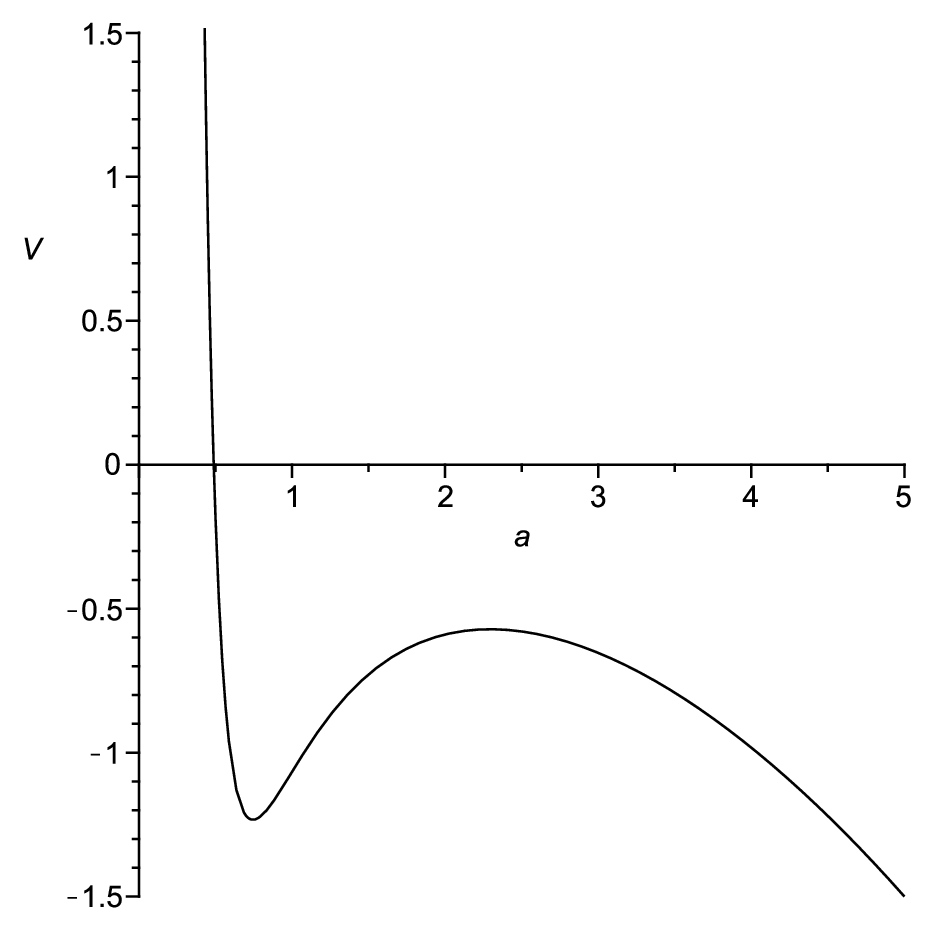
In order to see qualitative behavior of the system, let us rewrite the first integral (95) in the form of the energy conservation equation for a non-relativistic particle moving in a $1$ -dimensional potential as

\frac{1}{2}\dot{a}^{2}+\frac{2}{3\lambda-1}V(a)=0,

(96)

where

V(a)=\frac{\alpha_{3}K^{3}}{6a^{4}}+\frac{\alpha_{2}K^{2}}{2a^{2}}+\frac{K}{2}-\frac{\Lambda}{6}a^{2}-\frac{4\pi G}{3}\left[\rho a^{2}+\frac{C(t)}{a}\right].

(97)

The shape of the potential $V(a)$ completely determines the behavior of the system.

4.2.2 Simple examples

Let us now consider some simple examples. For simplicity we set $\alpha_{3}=1$ , $\alpha_{2}=0$ , $K=1$ , $\rho=0$ , $C=const$ . We still have freedom to choose values of $\Lambda$ and $C$ . We show four examples of the $1$ -dimensional potential (97): a bouncing universe (Figure 2), a cyclic universe (Figure 2), an unstable static universe (Figure 4) and a stable static universe (Figure 4). See [25] for more examples with $\rho=0$ and $C=const$ .

Refer to caption — Figure 1: $V(a)$ for $\Lambda=0.4$ and $8\pi GC=10$ . If the universe is initially contracting then it bounces and expands.

4.3 Scale-invariant cosmological perturbations from $z=3$ scaling

One of the essential ingredients of Hořava-Lifshitz gravity is the anisotropic scaling with the dynamical critical exponent $z\geq 3$ . Indeed, it is this property that makes the theory power-counting renormalizable and attractive as a candidate for the theory of quantum gravity. There are interesting cosmological implications of the anisotropic scaling. In this section we show that the anisotropic scaling with the minimal $z$ , i.e. $z=3$ , leads to a new mechanism for the generation of scale-invariant cosmological perturbations. Intriguingly, this mechanism works even without inflation.

4.3.1 Usual story with $z=1$

Before explaining the new mechanism, let us remind ourselves of the usual story with $z=1$ .

Cosmological perturbations are analyzed by perturbative expansion around a FRW background. In the linearized level, perturbations are Fourier expanded and the evolution of each mode is characterized by the frequency $\omega$ defined by the dispersion relation

\omega^{2}=c_{s}^{2}\frac{k_{c}^{2}}{a^{2}},

(98)

where $c_{s}$ is the sound speed, $k_{c}$ is the comoving wave number and $a$ is the scale factor of the universe. For simplicity we assume that the time dependence of $c_{s}$ , if any, is slow compared with the cosmological time scale $H^{-1}$ , where $H=\dot{a}/a$ is the Hubble expansion rate. (For example, $c_{s}$ is identically $1$ for a canonical scalar field with any potential.)

If a mode of interest satisfies $\omega^{2}\gg H^{2}$ then the evolution of the mode is not affected by the expansion of the universe and the mode just oscillates. When $\omega^{2}\ll H^{2}$ , on the other hand, the expansion of the universe is so rapid that the Hubble friction freezes the mode and the mode stays almost constant. Generation of cosmological perturbations from quantum fluctuations is nothing but the oscillation followed by the freeze-out. Therefore, the condition for generation of cosmological perturbations is

\frac{d}{dt}\left(\frac{H^{2}}{\omega^{2}}\right)>0.

(99)

With the $z=1$ dispersion relation (98), this condition is equivalent to $\ddot{a}>0$ for expanding universe ( $\dot{a}>0$ ). Therefore, if $z=1$ then generation of cosmological perturbations from quantum fluctuations requires accelerated expansion of the universe, i.e. inflation. For example, for power law expansion $a\propto t^{p}$ , $p>1$ is required.

Observational data of the cosmic microwave background strongly indicates that the primordial cosmological perturbations have an almost scale-invariant spectrum. It is easy to see that the scale-invariance also requires inflation. From the scaling (2) with $s=1$ , the amplitude of quantum fluctuations of the scalar field should be proportional to the energy scale of the system. In cosmology the energy scale is set by the Hubble expansion rate $H$ . Thus, we expect that

\delta\phi\propto H.

(100)

Since cosmological perturbations with different scales are generated at different times, the scale-invariance is nothing but the constancy of the right hand side of (100). Noting that $H=\dot{a}/a$ , this implies the exponential expansion of the universe $a\propto\exp(Ht)$ , namely inflation.

We have seen that, for $z=1$ , both the generation of cosmological perturbations and the scale-invariance of generated perturbations require the existence of an inflationary epoch in the early universe.

4.3.2 The story in the UV with $z=3$

The condition (99) for generation of cosmological perturbations is valid irrespective of the dispersion relation. In Hořava-Lifshitz gravity, to realize the anisotropic scaling (5), the dispersion relation for a physical degree of freedom in the UV should be

\omega^{2}=M^{2}\times\left(\frac{k_{c}^{2}}{M^{2}a^{2}}\right)^{z},

(101)

where $M$ is some energy scale. By substituting this to the condition (99) we obtain $d^{2}(a^{z})/dt^{2}>0$ for expanding universe ( $\dot{a}>0$ ). Since $z\geq 3$ in Hořava-Lifshitz gravity at high energy, generation of cosmological perturbations from quantum fluctuations does not require accelerated expansion of the universe, i.e. inflation. For example, power law expansion $a\propto t^{p}$ with $p>1/z$ satisfies the condition.

In this way, the anisotropic scaling provides a solution to the horizon problem. Essential reason for this is that perturbations freeze-out not at the Hubble horizon but at the sound horizon, defined by $\omega\sim H$ . The physical radius of sound horizon is thus $\sim(M^{z-1}H)^{-1/z}$ . In the UV epoch ( $H\gg M$ ), the sound horizon is far outside the Hubble horizon and can therefore accommodate scales much longer than the Hubble horizon size. In order to stretch microscopic scales to cosmological scales, we just need to have a long enough expansion history (satisfying the condition $d^{2}(a^{z})/dt^{2}>0$ ) in the UV epoch. Note that $M$ is not a cutoff scale of a low energy effective theory but is just the scale at which the theory starts exhibiting the anisotropic scaling, provided that Hořava-Lifshitz gravity is UV complete.

For general $z$ , the formula (7) implies that the amplitude of quantum fluctuations of $\phi$ should be

\delta\phi\sim M\times\left(\frac{H}{M}\right)^{\frac{3-z}{2z}},

(102)

where $M$ is defined through the dispersion relation (101). This is of course consistent with the well-known result (100) for $z=1$ and the result in ghost inflation $\delta\phi\sim(M^{3}H)^{1/4}$ [26, 27] for $z=2$ . On the other hand, in Hořava-Lifshitz gravity with the minimal value of $z$ ,i.e. $z=3$ , (102) is reduced to $\delta\phi\sim M$ , implying that the amplitude of quantum fluctuations does not depend on the Hubble expansion rate. This means that the spectrum of cosmological perturbations in Hořava-Lifshitz gravity with $z=3$ is automatically scale-invariant even without inflation.

4.3.3 A simple model

We have shown that the anisotropic scaling with $z=3$ naturally leads to a new mechanism for generation of scale-invariant cosmological perturbations. As a simple implementation of the mechanism, let us consider a free scalar field described by the action

I=\frac{1}{2}\int dtd^{3}\vec{x}N\sqrt{g}\left[\frac{1}{N^{2}}(\partial_{t}\phi-N^{i}\partial_{i}\phi)^{2}+\phi{\cal O}\phi\right],

(103)

where

{\cal O}=\frac{\Delta^{3}}{M^{4}}-\frac{\kappa\Delta^{2}}{M^{2}}+c_{\phi}^{2}\Delta-m_{\phi}^{2},\quad\Delta=g^{ij}D_{i}D_{j}

(104)

This is a covariantized version of (9).

In the UV, the first term in ${\cal O}$ is dominant and the scalar field action exhibits the $z=3$ scaling. In this regime it is easy to find the mode function in a flat FRW background as [5]

\phi_{\vec{k}_{c}}=\frac{e^{i\vec{k}_{c}\cdot\vec{x}}}{(2\pi)^{3}}\times 2^{-1/2}k_{c}^{-3/2}M\exp\left(-i\frac{k_{c}^{3}}{M^{2}}\int\frac{dt}{a^{3}}\right),

(105)

where $a$ is the scale factor, $t$ is the proper time, $\vec{k}_{c}$ is the comoving wave number and $k_{c}=|\vec{k}_{c}|$ . Note that this is not just WKB approximation but actually exact and applicable to both subhorizon and superhorizon scales in any background $a(t)$ , provided that the first term in ${\cal O}$ is dominant. The mode function approaches a constant value in the $a\to\infty$ limit if and only if the integral $\int^{\infty}dt/a^{3}$ converges. For power-law expansion $a\propto t^{p}$ , this condition is satisfied if $p>1/3$ , and agrees with the condition for the freeze-out after oscillation discussed after (101). Provided that the integral converges, the power-spectrum is calculated as

{\cal P}_{\phi}=\frac{k_{c}^{3}}{2\pi^{2}}\left|(2\pi)^{3}\phi_{\vec{k}_{c}}\right|^{2}=\left(\frac{M}{2\pi}\right)^{2}.

(106)

This is manifestly scale-invariant in accord with the general argument after (102). In this way, scale-invariant cosmological perturbations of the scalar field can be generated even without inflation.

After scales of interest exit the sound horizon, cosmological perturbations of the scalar field can be converted to curvature perturbations by either curvaton mechanism or modulated decay of heavy particles or/and oscillating fields. For example, it is possible to suppose that the scalar field $\phi$ itself plays the role of a curvaton [5]. When the Hubble expansion rate becomes as low as $m_{\phi}$ , $\phi$ starts rolling and eventually decays to radiation. Perturbations of $\phi$ are converted to those of radiation energy density and thus curvature perturbations.

In the IR, the first two terms in ${\cal O}$ can be neglected and the usual $z=1$ scaling is recovered. In this epoch, unless the universe is in an inflationary phase, physical scales re-enter the horizon as usual.

5 Summary and discussions

We have reviewed basic construction and cosmological implications of a power-counting renormalizable theory of gravitation recently proposed by Hořava. While there are many fundamental issues to be addressed in the future, it is interesting to investigate cosmological implications.

Since the high energy behavior of Hořava-Lifshitz gravity is very different from general relativity, there is a possibility that the theory does not exactly recover general relativity at low energy. As reviewed in subsection 4.1, this is indeed the case and the theory can instead mimic general relativity plus dark matter. The constraint algebra in this theory is smaller than general relativity since the time slicing is synchronized with the “dark matter rest frame” in the theory level. In subsection 4.2 we have shown that higher spatial curvature terms in the action drastically change the evolution of the early universe. We have derived modified Friedmann equation with higher spatial curvature terms and have shown some simple examples, including bouncing and cyclic universes. The anisotropic scaling at high energy is one of essential ingredients of the theory since the power-counting renormalizability stems from it. In subsection 4.3 we have reviewed a new mechanism for generation of cosmological perturbations based on the anisotropic scaling. This mechanism can solve the horizon problem and generate scale-invariant cosmological perturbations even without inflation.

In Sec. 3 we have commented on some issues related to the scalar graviton and the $\lambda\to 1+0$ limit, where $\lambda$ is a parameter in the kinetic action. We have explicitly seen that the naive metric perturbation breaks down for the scalar graviton in the $\lambda\to 1+0$ limit. However, this does not necessarily imply the loss of predictability. Actually, for spherically-symmetric, static, vacuum configurations we have proved that the limit is non-perturbatively continuous and safely recovers general relativity.

Now let us compile a list of some important open questions.

•

Renormalizability must be shown beyond power-counting argument. (See [28] for discussion about renormalizability of the theory with the detailed balance condition.)
•

The RG flow of the theory must be analyzed. In particular, it is very important to see whether $\lambda=1$ is an IR fixed point or not. If it is the case then we would like to know whether the RG flow can satisfy the condition (56) or not.
•

We have to develop mechanisms or symmetries to suppress Lorentz violating operators in the matter sector at low energies. Perhaps, embedding into a larger theory is needed. One such possibility is related to supersymmetry [16].
•

Is there an analogue of Vainshtein effect [11]? In subsection 3.4, non-perturbative continuity of the $\lambda\to 1+0$ limit was shown only for spherically-symmetric, static, vacuum configurations. We need to consider more general situations in order to see how general the non-perturbative continuity is.
•

In [10], based on exact results in some simple cases, it was conjectured that there is no caustic for constant time hypersurfaces. We need to provide evidences for this conjecture in more general situations if a proof is difficult. Perhaps, numerical simulations similar to those in [29] are necessary.
•

In [23] it was proved that a spherically-symmetric solution should include a time-dependent region near the center. On the other hand, as shown in Sec. 3 of the present article, the vacuum region far from the center recovers the standard Schwarzschild geometry. Since the size of the dynamical region is expected to be of the fundamental scale, the dynamical nature of the central region is not really relevant for macroscopic objects such as astrophysical stars. Microscopically, however, this could be rather significant . We would like to know, e.g. the typical size of the dynamical region and the motion of its boundary.
•

As already stressed in [10], we need to know if microscopic lumps of “dark matter as an integration constant” can play the role of particles in usual dark matter models from macroscopic viewpoint. Interactions among them such as collisions and bounces need to be understood. At astrophysical scales, we need to see if collective behavior of a group of large number of microscopic lumps can more or less mimic behavior of a cluster of particles with velocity dispersion and vorticity. Clearly, detailed investigation is necessary to understand rich dynamics of “dark matter” from microscopic to macroscopic scales.
•

As shown in (81), “dark matter as an integration constant” is generated in the early universe even if it vanishes initially. This formula can be applied to superhorizon perturbations. Given a concrete model of the matter sector, therefore, it is straightforward to estimate the typical amplitude and spectrum of the “dark matter”. If a single physical degree of freedom is responsible for both the source term $Q$ in (81) and generation of curvature perturbations then it should be possible to realize adiabatic initial conditions for the late time evolution of perturbations. (See [30] for classical late time evolution.) It is worthwhile investigating this possibility in details.
•

The mechanism reviewed in subsection 4.3 generates scale-invariant cosmological perturbations without a need for inflation. It would be interesting to see whether renormalization effects such as anomalous dimension can break the exact scale-invariance and explain the observed spectral tilt.
•

In the early universe, it is expected that $\lambda$ should deviate from $1$ under the RG flow and that the scalar graviton can be treated perturbatively. Since the scalar graviton has the $z=3$ anisotropic scaling in the UV, it should also obtain the scale-invariant cosmological perturbations [31]. Provided that $\lambda=1$ is a stable IR fixed point of the RG flow, as the universe expands and the Hubble expansion rate decreases, $\lambda$ approaches $1$ and the perturbative treatment of the scalar graviton becomes invalid ⁵⁵ 5 Thus, the conventional cosmological perturbation scheme [32] probably breaks down for the scalar graviton in the $\lambda\to 1+0$ limit. Again, this does not necessarily imply loss of predictability but requires nonlinear analysis.. However, the result in subsection 3.4 suggests that the $\lambda\to 1+0$ limit may be non-perturbatively continuous. A natural question is then “how to convert the scale-invariant cosmological perturbations of the scalar graviton to observables such as cosmic microwave background anisotropies and matter power spectrum?”

Since Hořava’s original proposal in January 2009, several extensions appeared in the literature. Blas, et.al. [21] proposed an extension without the projectability condition by including spatial derivatives of the lapse in the action. More recent proposal by Hořava and Melby-Thompson [33] respects the projectability condition but the fundamental symmetry of the theory is larger than the original one.

Throughout this article, we have considered the minimal theory, i.e. the original theory with the projectability condition but without extension of the symmetry. Whether this minimal theory is viable is still an open question and crucially depends on non-perturbative nature of the scalar graviton (see subsection 3.4) and properties of the RG flow (see the condition (56) ).

Acknowledgments

The author would like to thank Keisuke Izumi, Takeshi Kobayashi, Satoshi Maeda, Kazunori Nakayama, Tetsuya Shiromizu, Fuminobu Takahashi and Shuichiro Yokoyama for fruitful collaboration on this subject. He is grateful to Frans Klinkhamer, Massimo Porrati, Valery Rubakov, Misao Sasaki, Masaru Shibata and Takahiro Tanaka for useful discussions. The work of the author is supported by JSPS Grant-in-Aid for Young Scientists (B) No. 17740134, JSPS Grant-in-Aid for Creative Scientific Research No. 19GS0219, MEXT Grant-in-Aid for Scientific Research on Innovative Areas No. 21111006, JSPS Grant-in-Aid for Scientific Research (C) No. 21540278, and the Mitsubishi Foundation. This work was supported by World Premier International Research Center Initiative.

References

[1] P. Horava, Phys. Rev. D 79, 084008 (2009) [arXiv:0901.3775 [hep-th]].
[2] G. Calcagni, JHEP 0909, 112 (2009) [arXiv:0904.0829 [hep-th]].
[3] R. Brandenberger, Phys. Rev. D 80, 043516 (2009) [arXiv:0904.2835 [hep-th]].
[4] E. Kiritsis and G. Kofinas, Nucl. Phys. B 821, 467 (2009) [arXiv:0904.1334 [hep-th]].
[5] S. Mukohyama, JCAP 0906, 001 (2009) [arXiv:0904.2190 [hep-th]].
[6] S. Maeda, S. Mukohyama and T. Shiromizu, Phys. Rev. D 80, 123538 (2009) [arXiv:0909.2149 [astro-ph.CO]].
[7] S. Mukohyama, K. Nakayama, F. Takahashi and S. Yokoyama, Phys. Lett. B 679, 6 (2009) [arXiv:0905.0055 [hep-th]].
[8] T. Takahashi and J. Soda, Phys. Rev. Lett. 102, 231301 (2009) [arXiv:0904.0554 [hep-th]].
[9] S. Mukohyama, Phys. Rev. D 80, 064005 (2009) [arXiv:0905.3563 [hep-th]].
[10] S. Mukohyama, JCAP 0909, 005 (2009) [arXiv:0906.5069 [hep-th]].
[11] A. I. Vainshtein, Phys. Lett. B 39, 393 (1972).
[12] M. Fierz and W. Pauli, Proc. Roy. Soc. Lond. A 173, 211 (1939).
[13] M. Ackermann et al. [Fermi GBM/LAT Collaborations], Nature 462, 331 (2009) [arXiv:0908.1832 [astro-ph.HE]]. For the limits on $M_{QG,2}$ relevant for the parity and time-reversal invariant dispersion relation, see the supplementary material at http://gammaray.nsstc.nasa.gov/gbm/grb/GRB090510/supporting_material.pdf.
[14] J. Albert et al. [MAGIC Collaboration and Other Contributors Collaboration], Phys. Lett. B 668, 253 (2008) [arXiv:0708.2889 [astro-ph]].
[15] R. Iengo, J. G. Russo and M. Serone, JHEP 0911, 020 (2009) [arXiv:0906.3477 [hep-th]].
[16] S. Groot Nibbelink and M. Pospelov, Phys. Rev. Lett. 94, 081601 (2005) [arXiv:hep-ph/0404271].
[17] T. P. Sotiriou, M. Visser and S. Weinfurtner, Phys. Rev. Lett. 102, 251601 (2009) [arXiv:0904.4464 [hep-th]].
[18] C. Charmousis, G. Niz, A. Padilla and P. M. Saffin, JHEP 0908, 070 (2009) [arXiv:0905.2579 [hep-th]].
[19] M. Henneaux, A. Kleinschmidt and G. L. Gomez, Phys. Rev. D 81, 064002 (2010) [arXiv:0912.0399 [hep-th]].
[20] A. Wang and R. Maartens, Phys. Rev. D 81, 024009 (2010) [arXiv:0907.1748 [hep-th]].
[21] D. Blas, O. Pujolas and S. Sibiryakov, Phys. Rev. Lett. 104, 181302 (2010) [arXiv:0909.3525 [hep-th]].
[22] K. Koyama and F. Arroja, JHEP 1003, 061 (2010) [arXiv:0910.1998 [hep-th]].
[23] K. Izumi and S. Mukohyama, Phys. Rev. D 81, 044008 (2010) [arXiv:0911.1814 [hep-th]].
[24] C. Doran, Phys. Rev. D 61, 067503 (2000) [arXiv:gr-qc/9910099].
[25] K. i. Maeda, Y. Misonoh and T. Kobayashi, arXiv:1006.2739 [hep-th].
[26] N. Arkani-Hamed, H. C. Cheng, M. A. Luty and S. Mukohyama, JHEP 0405, 074 (2004) [arXiv:hep-th/0312099].
[27] N. Arkani-Hamed, P. Creminelli, S. Mukohyama and M. Zaldarriaga, JCAP 0404, 001 (2004) [arXiv:hep-th/0312100].
[28] D. Orlando and S. Reffert, Class. Quant. Grav. 26, 155021 (2009) [arXiv:0905.0301 [hep-th]].
[29] N. Arkani-Hamed, H. C. Cheng, M. A. Luty, S. Mukohyama and T. Wiseman, JHEP 0701, 036 (2007) [arXiv:hep-ph/0507120].
[30] T. Kobayashi, Y. Urakawa and M. Yamaguchi, JCAP 0911, 015 (2009) [arXiv:0908.1005 [astro-ph.CO]].
[31] B. Chen, S. Pi and J. Z. Tang, JCAP 0908, 007 (2009) [arXiv:0905.2300 [hep-th]].
[32] J. O. Gong, S. Koh and M. Sasaki, Phys. Rev. D 81, 084053 (2010) [arXiv:1002.1429 [hep-th]].
[33] P. Horava and C. M. Melby-Thompson, arXiv:1007.2410 [hep-th].

Hořava-Lifshitz Cosmology: A Review

Abstract

1 Introduction

2 Hořava-Lifshitz gravity

2.1 Preliminaries

2.1.1 Power-counting

2.1.2 Abandoning Lorentz symmetry

2.1.3 Scalar field action

2.2 Symmetry

2.3 Basic quantities and projectability condition

2.4 Action

2.4.1 The UV action

2.4.2 Relevant deformations in the IR

2.4.3 IR action with z=1z=1

2.5 Equations of motion

3 Scalar graviton and the λ→1+0\lambda\to 1+0 limit

3.1 Propagating degrees of freedom

3.2 Dispersion relation

3.3 Breakdown of metric perturbation

3.4 Non-perturbative continuity at λ=1+0\lambda=1+0

3.5 Schwarzschild solution and Newtonian limit

4 Cosmological implications

4.1 Dark matter as an integration “constant”

4.1.1 Structure of GR and FRW universe

4.1.2 Structure of HL gravity and FRW universe

4.1.3 General case in the IR

4.2 Bouncing and cyclic universes

4.2.1 Modified Friedmann equation with higher curvature terms

4.2.2 Simple examples

4.3 Scale-invariant cosmological perturbations from z=3z=3 scaling

4.3.1 Usual story with z=1z=1

4.3.2 The story in the UV with z=3z=3

4.3.3 A simple model

5 Summary and discussions

Acknowledgments

References

2.4.3 IR action with $z=1$

3 Scalar graviton and the $\lambda\to 1+0$ limit

3.4 Non-perturbative continuity at $\lambda=1+0$

4.3 Scale-invariant cosmological perturbations from $z=3$ scaling

4.3.1 Usual story with $z=1$

4.3.2 The story in the UV with $z=3$