Role of two-flavor color superconductor pairing in a three-flavor Nambu–Jona-Lasinio model with axial anomaly
Abstract
The phase diagram of strongly interacting matter is studied within a three-flavor Nambu–Jona-Lasinio model, which contains the coupling between chiral and diquark condensates through the axial anomaly. Our results show that it is essential to include the 2SC phase in the analysis. While this is expected for realistic strange quark masses, we find that even for equal up, down, and strange bare quark masses, 2SC pairing can be favored due to spontaneous flavor-symmetry breaking by the axial anomaly. This can lead to a rich phase structure, including BCS- and BEC-like 2SC and CFL phases and new endpoints. On the other hand, the low-temperature critical endpoint, which was found earlier in the same model without 2SC pairing, is almost removed from the phase diagram and cannot be reached from the low-density chirally broken phase without crossing a preceding first-order phase boundary. For physical quark masses no additional critical endpoint is found.
I Introduction
The phase diagram of strongly interacting matter is studied with great effort, both experimentally and theoretically. From direct observations we know that at low temperature and low chemical potential chiral symmetry is spontaneously broken and hadrons are the relevant degrees of freedom. There are strong indications from heavy-ion experiments that this is changed at high temperatures where quarks and gluons become the relevant degrees of freedom and a so-called quark-gluon plasma (QGP) is formed (see Ref. [1] for an overview). This is also confirmed by lattice simulations of quantum chromodynamics (QCD) at nonvanishing temperature [2, 3]. These calculations indicate that, for physical quark masses and vanishing chemical potential, the hadronic phase and the QGP are connected by a smooth crossover [4].
At high densities and low temperatures, on the other hand, strongly interacting matter is expected to be a color superconductor, where the quarks form Cooper pairs (for reviews, see [5, 6, 7, 8, 9, 10, 11]). This can rigorously be shown for asymptotically high densities by applying weak-coupling techniques to QCD [12, 13, 14, 15]. Unfortunately, these methods fail at more “moderate” densities, which are of phenomenological interest. Moreover, because of the “sign problem”, the regime of low temperature and nonvanishing chemical potential cannot be studied within lattice QCD. However, in model calculations one typically finds that the hadronic phase is bordered by a first-order phase boundary in the low-temperature region [16, 17]. The combination of this result with the notion of the crossover at zero chemical potential then leads to the standard picture of the phase diagram where the first-order phase transition ends at a critical end point (CEP). The latter has attracted considerable attention, as it is potentially detectable in heavy-ion experiments [18].
It is possible, however, that the phase boundary of the hadronic phase contains more than one CEP. For instance, it was found within a Nambu–Jona-Lasinio (NJL) model that imposing charge neutrality or the inclusion of vector interactions weaken the first-order phase transition and can lead to a second end point at low temperatures near the chemical potential axis [19, 20, 21]. Beside these mechanisms, it has been shown in a Ginzburg-Landau (GL) analysis [22, 23, 24] that the interaction between the chiral and diquark condensates, induced by the axial anomaly, can also lead to such a low-temperature endpoint. This result is rather general, but it strongly depends on the values of the GL coefficients, which could not be determined within this framework. It is therefore very interesting that it has recently been confirmed explicitly within an NJL-model study [25]. Thereby the authors have included a -symmetry breaking interaction term which connects chiral and diquark condensates. This term plays a crucial role in the GL analysis but is usually neglected in the NJL model. In it was found that it indeed leads to the emergence of a second CEP if the coupling is sufficiently strong.
However, the calculations have been performed under the simplifying assumption of three quark flavors with equal masses. In this case it appears natural that color superconducting quark matter is realized in the color-flavor locked (CFL) phase [26], where up, down, and strange quarks are paired in a very symmetric way. The authors of Ref. [25] have therefore considered only one common diquark condensate and one common chiral condensate in their analysis. The same is true for the GL analysis of Refs. [22, 23, 24] in the case of equal quark masses. Of course, the assumption of equal quark masses is quite unrealistic, leading to the question whether the second CEP can still be found in a scenario where the strange quark mass is significantly larger than the masses of the up and down quarks. In order to investigate this question, some generalizations of the model are necessary: When the quark masses are different, the chiral condensates will take different values for different flavors and also the diquark condensates will depend on the flavor content of the paired quarks. In particular, at large differences between strange and nonstrange quark masses, the CFL pairing will become unfavored [27, 28, 29] and a two-flavor color superconductor (2SC) [30, 31] will emerge, where only up and down quarks are paired.
In the following we will analyze the effect of these generalizations on the phase structure. Thereby it was our original motivation to investigate the effect of realistic mass differences. However, to our surprise, we find that even for equal bare quark masses the 2SC phase can be favored due to the coupling of the chiral and diquark condensates by the axial anomaly. As a result we find the scenario of Ref. [25] never to be favored, not even for equal quark masses.
II The model
II.1 The Lagrangian
We adopt the NJL-type Lagrangian of ,
| (1) |
which is based on a frequently used Lagrangian (e.g., [32, 33, 34, 35]), extended by the interaction term . It describes the dynamics of a quark field with three color (r,g,b) and three flavor (u,d,s) degrees of freedom. The current quark masses enter through the diagonal mass matrix and is the quark chemical potential. In the present analysis, we do not impose electric or color charge neutrality constraints. These constraints play an important role in compact stars and can lead to a rather complicated phase structure [32, 33, 34, 35, 36]. On the other hand, they are less important in heavy-ion collisions, where the matter does not need to be locally neutral. As a first step, we therefore use a common chemical potential for all quarks, in order to keep the analysis simple.
The Lagrangian Eq. (1) includes a four-point interaction in the quark-antiquark channel,
| (2) |
and a four-point interaction in the quark-quark channel,
| (3) |
Here and are dimensionful coupling constants, is the charge conjugation matrix, and are the Gell-Mann matrices in flavor space, extended by . The flavor and color structure of the quark-quark interaction is generated by the antisymmetric matrices
| (4) |
where are the Gell-Mann matrices in color space.
The four-point interaction terms and are symmetric under transformations in flavor space. In order to break the axial symmetry we include the standard six-point interaction term [37, 38]
| (5) |
which can be related to instanton effects. This term connects three incoming right-handed fields with three outgoing left-handed fields, and vice versa. In principle, it can therefore couple to three quark-antiquark channels (e.g., ) as well as to one quark-antiquark channel together with one diquark and one anti-diquark (e.g., ). However, in Hartree approximation, which will be employed below, only connects quark-antiquark condensates but no diquark condensates. Since on the other hand the coupling between quark-antiquark and diquark condensates was found to be important in the GL analysis of Refs. [22, 23, 24], the authors of have introduced a second six-point interaction. In our notation, Eq. (4), this term can be written as
| (6) |
where in the last factor the indices and refer to the flavor components. has the same symmetries as Eq. (5) but the quark fields are ordered in such a way that in Hartree approximation the diquark and quark-antiquark condensates are connected. This reordering of the quark fields can be realized via a Fierz transformation,11 1 Useful references in this context are Refs. [39, 40, 41]. of the instanton vertex, relating to . In this way one can also relate the new coupling constant to . However, following , we will treat as a free independent parameter.
II.2 Mean-field approximation and thermodynamic potential
We are working in mean-field approximation by introducing the scalar diquark condensates
| (7) |
and the scalar antiquark-quark condensates
| (8) |
In Hartree approximation the six-point interaction , Eq. (6), then is simplified to
| (9) |
One can identify the first term as a contribution to the effective quark masses, while the following two terms contribute to the anomalous selfenergy of the propagator in the color superconducting phase. The last term does not depend on the fields and gives a constant contribution.
Adding the other terms from Eq. (1) and using Nambu-Gorkov bispinors the full mean-field Lagrangian can be written as
| (10) |
with the inverse dressed propagator
| (11) |
Here is the diagonal mass matrix of the constituent quark masses with the components
| (12) |
The off-diagonal elements of Eq. (11) include
| (13) |
Finally includes a field-independent term
| (14) |
With these ingredients the thermodynamic potential in mean-field approximation becomes
| (15) |
where the sum is over fermionic Matsubara frequencies. For equal diquark condensates, , and equal chiral condensates, , it agrees with the thermodynamic potential of , where only this limit was considered.
The self-consistent mean-field solutions are given by the stationary points of with respect to the condensates, i.e., by the solutions of the gap equations
| (16) |
The phase diagram is then constructed by taking the solution with the highest pressure (i.e., the lowest value of ) at each point in the - plane.
II.3 Parameters
The model defined above contains eight parameters: the three bare quark masses (), the two four-point coupling constants (), the two six-point coupling constants (), and a regularization parameter. For the latter we take a sharp three-momentum cut-off .
To fix these parameters, we basically follow the procedure of . Starting point are the parameters of ,
| (17) |
which have been obtained by fitting meson masses and decay constants in vacuum. The value of the quark-quark coupling , which cannot be determined from vacuum meson properties, is taken from ,
| (18) |
Finally, as already mentioned, we treat the coupling constant as a free parameter. We will often take , because with this value a second endpoint was found in .
The authors of have only studied the case of equal quark masses. To that end, they reduced the bare strange quark mass to the value of the up and down quark masses and then re-adjusted the antiquark-quark coupling , so that the dynamical up and down quark masses remain unchanged in vacuum (parameter set II of ):
| (19) |
In this way the vacuum values of the chiral condensates and of the pion mass and decay constant remain unchanged as well.
Since we are interested in the effect of the strange quark mass on the phase structure we generalize this procedure to the case of arbitrary values of . Starting with equal quark masses, Eq. (19), we will increase the bare strange quark mass up to the more realistic case, Eq. (17), always keeping the dynamical vacuum masses fixed by adjusting the coupling constant .
III Results
In this section we present our numerical results, which mainly consist of a series of phase diagrams with different six-point couplings and different choices for the strange quark mass. We begin with the case of equal bare quark masses in Sec. III.1, before introducing larger values of in Sec. III.2.
III.1 Equal bare masses

As a basis for our investigations, we consider equal quark masses, and allow for only one common chiral condensate and one common diquark . For we then reproduce the phase diagram obtained in , as shown in Fig. 1. The normal phases, where all diquark condensates vanish, are denoted by ‘SB’ in regions with large chiral condensates and by ‘NQ’ in regions with small chiral condensates. At low chemical potential and high temperature these two regions are connected by a crossover, while at higher chemical potential and lower temperature they are separated by a first-order phase boundary. Without diquark condensates the latter would continue down to the chemical-potential axis. However, when diquark condensates are included, the CFL phase is favored in the lower right part of the phase diagram, replacing the NQ phase in that regime. The first-order chiral phase transition then does no longer go down to zero temperature but ends inside the CFL phase,22 2 In this article we use the term ‘chiral phase transition’ whenever the transition is mainly characterized by a change of the chiral condensates . Note, however, that in the CFL phase chiral symmetry is always broken by the diquark condensates. while the latter is bordered to the SB phase by a second-order phase boundary.
As discussed in , this particular phase structure is a consequence of the interaction term . Without this term, i.e., for , the SB-CFL phase transition is first order and basically a continuation of the first-order SB-NQ phase transition (see Fig. 4 below). In particular, the chiral condensate drops considerably at the phase boundary and is therefore small in the entire CFL phase. This is different for sufficiently large values of , as in Fig. 1. In this case the coupling between chiral and diquark condensates leads to the existence of strongly bound diquarks in the SB phase, which eventually condense and then form a Bose-Einstein condensate (BEC) in the lower- part of the CFL phase (see also ). Hence, the SB-CFL phase boundary is simply the condensation line of the diquarks and therefore the transition is continuous. In particular, the chiral condensate is still large at the phase boundary and only decreases considerably at somewhat higher values of . In a small regime near the boundary to the NQ phase this happens discontinuously and is just the continuation of the first-order phase transition between the SB and the NQ phase. At most temperatures, however, the decrease is continuous and closely related to a BEC-BCS crossover where the BEC-like CFL phase (‘’) gets converted into a BCS-like CFL phase (‘’). The corresponding crossover line is indicated in the figure as well. Following we have defined it as the line where the in-medium constituent quark masses are equal to . Note that with this definition the crossover line does not exactly run into the endpoint of the first-order phase boundary.

Next we allow the different diquark condensates and the chiral condensates to vary independently for . This opens the possibility for the formation of a 2SC phase (). Still keeping the bare quark masses equal, we obtain the phase diagram shown in Fig. 2. Whereas the normal-conducting phases NQ and SB occupy approximately the same regions of the phase diagram as in Fig. 1, we find that a large part of the CFL phase is replaced by a 2SC phase. The first-order chiral phase transition, which in Fig. 1 ends inside the CFL phase, now separates a BEC-like 2SC phase with large chiral condensates (‘’) and a BCS-like 2SC phase with small chiral condensates (‘’). However, unlike in Fig. 1, the BEC-like and the BCS-like phases are always separated by a first-order phase transition and never connected by a crossover.
Since and vanish in the 2SC phase whereas they are equal to in the CFL phase, the two phases are necessarily separated by first-order phase boundaries. On the other hand, the phase transition from the CFL phase as well as from the neighboring region of the 2SC phase to the NQ phase is of second order.33 3 For simplicity, we drop the subscripts ‘BCS’ or ‘BEC’ when the distinction between BCS-like or BEC-like phases is not relevant for the discussion. As an interesting consequence, the first-order 2SC-CFL phase-transition line ends exactly on the second-order phase boundary to the NQ phase. Also note that the 2SC-NQ phase boundary, in the regime where it is second order, exactly agrees with the CFL-NQ phase boundary in Fig. 1. This is due to the fact that on the second-order phase boundary all diquark condensates vanish and therefore the 2SC phase and the CFL phase have the same free energy. For similar reasons the second-order SB- phase boundary agrees with the SB- phase boundary in Fig. 1. Again, this is not surprising because both boundaries are related to the Bose-Einstein condensation of diquarks, which are identical in the SB phase and, hence, on the boundary.
At low temperatures () we find a small area between the phase and the phase, where the phase is slightly preferred. The origin of this “CFL island” will become more clear below.

In order to get a more complete picture, we now vary the coupling constant of the six-point interaction . In Fig. 3 we show the phase diagram in the - plane for . One immediately recognizes that for all choices of there is always a first-order phase transition at some value of . For low values of only the SB phase and the CFL phase are present. The first interesting development occurs when the interaction gets strong enough to have bound diquarks in the SB phase, which then condense at some value of . As a consequence, a phase appears in the phase diagram. At a slightly higher value of the CFL phase splits into a BEC-like and a BCS-like region. These two regimes are separated by a first-order transition, which eventually turns into a crossover at higher values of . The corresponding endpoint marks the critical value of where in the phase diagram with equal condensates (, ) the lower critical end point appears on the -axis. However, allowing for 2SC pairing, there still is a first-order transition between the and the phase.
Cutting Fig. 3 at , we reproduce the behavior of Fig. 2. From this perspective it becomes clear that the “CFL island”, which we have found there between the and the phase, corresponds to the upper end of the regime and will disappear at a slightly higher value of .


In Fig. 4 we show a series of phase diagrams in the - plane in order to illustrate how the phase structure evolves with . While the effect is almost negligible for small and moderate values of , a major restructuring takes place at : It starts with a phase, which appears near the triple point of the three original phases (b) and then grows towards lower temperatures and higher chemical potentials. Slightly below , Bose condensation of diquarks sets in, leading to a phase and shortly afterwards to a phase (c). At the beginning, the latter is completely separated from the phase by a first-order phase boundary, which turns into a crossover upon further increasing . As a result we find at a critical endpoint (d), which is of the same origin as the low-temperature critical endpoint in Fig. 1. Note, however, that the endpoint is now located in a region which is separated from the low-density regime by a first-order phase transition between 2SC and CFL phase. Moreover, the endpoint exists only in an extremely small interval of the coupling : While for the - phase transition is still first order down to , already at the entire phase boundary including the endpoint is covered by the 2SC phase. Eventually, the latter reaches the -axis and the two CFL regimes become separated again (e). At even higher , the first-order - phase transition turns into a crossover, leading to another endpoint (f).44 4 As mentioned earlier, the BEC-BCS cross-over line (blue dotted line), which we have defined as the line where the non-strange constituent quark masses are equal to , does not exactly run into the endpoint. In this sense, the first-order phase transition (related to a discontinuity in the condensates) does not exactly coincide with the BEC-BCS transition, although both are closely related to each other. This endpoint is located at the upper temperature end of the first-order boundary, like the “conventional” endpoint of the SB-NQ phase boundary, and it moves downwards with increasing . Finally, slightly above , it reaches the -axis and only a crossover remains (not shown). On the other hand, as argued before, the 2SC-CFL phase transition is necessarily first order, and therefore there is always a discontinuous phase transition at low temperatures.
After getting this overview, we would like to understand how the 2SC phase can be preferred over the CFL phase in some regions of the phase diagram although we have chosen equal bare quark masses. It clearly means that the -flavor symmetry is spontaneously broken, so there is in fact a continuous set of degenerate ground states, which are related to each other by flavor rotations. Bearing in mind that we will introduce larger strange quark masses later on, we choose, without loss of generality, the standard 2SC pairing pattern, i.e., , .
As obvious from Figs. 3 and 4, the emergence of the 2SC phase at equal bare quark masses is a consequence of the six-point interaction . This term couples the chiral condensates to the diquark condensates and, thus, the constituent quark masses to the diquark gaps, see Eqs. (12) and (13). However, whereas in the CFL phase this happens symmetrically for all flavors, in the 2SC phase these equations conspire in a rather peculiar way: Since but , there is a contribution from the diquark condensates to but not to and . Hence, even if we start with equal bare quark masses, in the 2SC phase the strange quarks will be heavier than the non-strange quarks. In turn, the larger value of leads to an enhancement of via an increased modulus of the (negative) condensate in Eq. (13).
This effect is illustrated in Fig. 5, where the diquark gap parameters and the constituent quark masses are shown as functions of the six-point coupling strength for the CFL and 2SC solutions at and . One can clearly see that and in the 2SC phase rise much faster with than the other quantities shown in the figure. In particular the ratio between in the 2SC phase and the common gap parameter in the CFL phase rises from about 1.25 at to 2.0 at . It is therefore plausible that eventually the gain in free energy is larger for 2SC pairing than for CFL pairing. In fact, if we had only diquark condensates and no dynamical quark masses, the pairing energy would be proportional to for each quasiparticle mode with pairing gap . 2SC pairing would then be favored for . Although in our case the dynamical quark masses (and their coupling to the diquark condensates) are crucial and certainly cannot be neglected, this estimate can at least roughly explain the numerical results.


At first sight the results found in this section seem to contradict the GL anlysis of Refs. [22, 23, 24] where no 2SC-like solution was found for three equal flavors. However, although starting from a general GL potential, the authors have chosen a particular ansatz for the condensates which does not allow for such solutions. By making a more general ansatz one can show that our results are indeed consistent with the GL analysis. This is discussed in more detail in App. A.
III.2 Realistic strange quark mass

We now introduce bare strange quark masses that are larger than the masses of the up and down quarks. In particular we are interested in , which is the value obtained in by fitting vacuum meson properties. We begin, however, with a more systematic investigation of the mass effects by gradually increasing from the equal-mass case to the “realistic” value . Thereby we adjust the coupling for each value of as described in Sec. II.3.
The phase diagram in the - plane at for is shown in Fig. 6. As usual, we now define the CFL phase as a phase where all three diquark gaps take nonvanishing values but do not need to be equal. With rising , since pairs involving strange quarks become increasingly disfavored, the CFL phase gets more and more replaced by the 2SC phase, thus pushing the phase boundary to higher values of . As the spontaneous breaking of flavor through the mechanism described above is now stabilized by an explicit symmetry breaking, even a small enhancement of has a rather large effect. For similar reasons, the small CFL area between the phase and the phase disappears already at . Above this point there is a first-order phase transition between the two 2SC phases, which ends at .
A larger value of also leads to a larger value of the strange chiral condensate , which in turn leads to an enhancement of the effective four-point quark-quark coupling in the channel. The latter comes about from closing a strange-quark loop in the six-point interaction term and adding this contribution to the genuine four-point vertex from . As a consequence, the diquarks get bound more deeply, i.e., the diquark mass is reduced and, hence, their condensation, which determines the transition from the SB phase to the phase is shifted to lower quark chemical potential.

In the remaining part of this article, we fix the strange quark mass at the “realistic” value, . In Fig. 7 we show the phase structure at T = 0 in dependence of the six-point coupling strength . With increasing the effective quark-quark coupling becomes stronger and the SB-2SC phase transition moves to lower quark chemical potentials. Around the phase forms at the low chemical potential side of the chiral phase transition line. With larger this region becomes broader and at the first-order phase transition between the phase and the phase ends. Similar to the equal-mass case we also find that an increase of is more favorable for the 2SC phase than for the CFL phase, so that the latter gets shifted to higher values of .


In Fig. 8, we finally show a series of phase diagrams in the - plane for different values of . A general result is that none of them contains a critical endpoint at the low-temperature side of the first-order chiral phase transition. For we recover the standard phase diagram (a), which has been calculated, e.g., in Ref. [29] for the same parameters: At low temperature chiral symmetry is restored in a first-order phase transition between SB and 2SC phase, which is continued by a first-order phase transition between SB and NQ phase at higher temperatures and finally ends in a critical endpoint. Furthermore, there is a CFL phase at low temperature and high chemical potential. With increasing the 2SC pairing becomes strengthened so that the CFL phase is pushed to higher chemical potentials while the first-order chiral phase transition gets successively “swallowed” by the expanding 2SC phase: As a first step the upwards-moving second-order 2SC-NQ phase boundary reaches the critical endpoint of the SB-NQ phase boundary (b). Next, a phase emerges on the left-hand-side of the SB-2SC phase boundary (c,d) and eventually the condensation line unites with the -NQ phase boundary (e). At the same time first-order chiral symmetry restoration line becomes disconnected and ends inside the 2SC phase. When is further increased, the endpoint moves downwards in temperature and finally disappears completely (f).
IV Conclusions
We have investigated the phase structure of strongly interacting matter within a three-flavor NJL-type model with an extended six-point interaction that couples chiral and diquark condensates. This interaction term, which is usually neglected in NJL-model studies of the phase diagram, has been introduced in and mimics effects of the axial anomaly. While this in principle leads to a more complete picture, the corresponding coupling constant is basically unknown and was therefore treated as a free parameter in our analysis.
Aim of the present study was to extend the investigations of to realistic strange quark masses. In this context we have generalized the mean-field ansatz to allow for flavor-dependent chiral and diquark condensates. This opens the possibility for 2SC pairing, which was expected to become relevant at large strange quark masses.
It turned out, however, that even for equal bare quark masses the 2SC phase is present in the phase diagram if the coupling is sufficiently strong. This spontaneous breaking of the flavor symmetry occurs because the axial anomaly induces a mutual amplification of the strange chiral condensate and the non-strange diquark condensate. As an important consequence, we have not found a continuous transition from the low-density chirally broken phase to the CFL phase at for any value of between and . Related to this, the low-temperature critical end point which was found in only survives in an extremely narrow interval and is otherwise covered by the 2SC phase.
As expected, the 2SC phase plays an even more important role at larger bare strange quark masses, in particular for the “realistic value”, taken from a fit to vacuum observables. By varying we find several qualitatively different phase diagrams, where the first-order chiral phase transition ends outside, inside or on the phase boundary of the 2SC phase or where there is no first-order chiral phase transition at all. It should be noted, however, that most of these qualitative changes only occur at relatively large values of , which may turn out to be unrealistic. But even for smaller couplings, the anomaly can be quantitatively important, as it stabilizes the 2SC pairing and shifts the CFL phase to higher chemical potentials.
The present study may be seen as a minimal extension of the analysis of to include realistic strange quark masses. There are, however, many other aspects which have not yet been taken into account. Perhaps most important is the consideration of inhomogeneous phases. For a two-flavor NJL model without color superconductivity it has been shown that the entire first-order chiral phase transition line is covered by an inhomogeneous region and therefore removed from the phase diagram [44, 45, 46]. It would be interesting to see how this result is modified when strange quarks and color superconducting phases are included and how the results depend on the axial anomaly.
We have also neglected the possibility of kaon condensation in the CFL phase [47], which was found to be very important in an NJL model with realistic strange quark masses [34, 35]. In these references, on the other hand, the anomaly effects described by have not been taken into account. This term should lead to a higher kaon mass and therefore suppress its condensation. It would be interesting to study this in more detail.
Finally, we should recall that we have restricted ourselves to a single quark chemical potential. Similar investigations of anomaly effects should also be performed for electrically and color neutral matter.
IV.1 Acknowledgments
The work of H.B. was supported by the Helmholtz International Center for FAIR and by the Helmholtz Graduate School for Hadron and Ion Research. M.B. acknowledges partial support by EMMI.
Appendix A Ginzburg-Landau approach
The most general expression for the GL free energy up to order four is given in the equations (7), (13) and (14) in as the difference to the normal phase
| (20) |
with
| (21) |
Here , and are matrices containing the chiral and the left- and right-handed diquark fields, respectively (for details, see ). This ansatz has 13 unkown coefficients which are in general and dependent functions and cannot be determined within the GL analysis.
For the investigation of three massless flavors the authors of have therefore restricted themselves to an ansatz with equal condensates for all flavors, and . The free energy then takes the simplified form
| (22) |
with only seven independent coefficients,55 5 In addition, a term of order must be introduced by hand in order to stabilize the system if . For simplicity, we neglect such terms in the present qualitative discussion. which are related to the original GL coefficients in Eq. (21) by
| (23) |
Yet, the full exploration of the remaining seven-dimensional parameter space would still be almost impossible. However, by making additional, physically motivated, assumptions (e.g., positivity of , , , and ) interesting non-trivial results have been extracted in Refs. [22, 23, 24].
Similarly, two-flavor systems have been investigated in choosing and , i.e., by completely neglecting all condensates which involve strange quarks. The resulting free energy is given by
| (24) |
with five independent coefficients, which are different from those in Eq. (22). In this context it is important to note that by neglecting the strange condensates completely, it was assumed that the strange quarks are infinitely heavy and therefore decouple from the non-strange sector. In particular, a direct comparison of with in order to study the competion between 2SC and CFL pairing was not intended and is not possible.
In contrast, in our NJL-model anlysis, we have studied a 2SC phase in a three-flavor environment with a large strange quark chiral condensate. The corresponding GL ansatz is and , yielding
| (25) |
where the coefficients , , , and are the same as in Eq. (23), and
| (26) | ||||||
Hence, instead of five GL coefficients as in Eq. (24), depends on nine independent coefficients. In particular, unlike , it contains the anomaly induced - and -terms which are related to the six-point interactions Eqs. (5) and (6) in the NJL-Lagrangian.
Obviously, the extra terms in Eq. (25) are due to the strange chiral condensate , which is not present in . We can thus recover Eq. (24) by setting equal to zero. In fact, a more appropriate way to describe the decoupling of the strange quarks with large masses is to treat as a nonvanishing constant. The -term, among others, then leads to a renormalization of the -coefficient , while, e.g., the -term leads to a shift of the vacuum energy. This underlines again that a diract comparison of the free energies obtained with and would be meaningless.
On the other hand, keeping as a dynamical variable, a comparison of with is possible.66 6 Here we tacitly assume that the GL anaysis is meaningful in both phases, i.e., that all condensates are small. Clearly, this does not need to be the case. To that end, we should replace the coefficient in Eq. (22) by the combination and the coefficient by . Moreover, we have to take into account that the coefficients and are linear independent (see Eqs. (23) and (26)). This can be accounted for by writing and with and . Thus, in oder to compare the free energies of the 2SC and CFL solutions, we have to deal with ten independent parameters77 7 A straightforward way to obtain a unified description of both, CFL and 2SC phase, is to make the ansatz and . In this case there are eleven independent coefficients. Our approach is more restrictive and therefore has one parameter less. (, , , , , , , , , ), plus possible six-order terms which might be needed for stability reasons. An exhaustive GL analysis is therefore practically impossible.
However, since we only want to show that 2SC-like solutions can indeed be favored in some cases, it is sufficient to demonstrate this by an example. In order to proceed, we therefore make a few simplifying assumptions: (i) We neglect all -terms, i.e, . This was also done in in the three-flavor case. (ii) In the NJL model without the anomaly terms and without diquark coupling, i.e., taking into account only the interaction term , the different flavors do not mix. Hence their contributions to the thermodynamic potential are additive. To reproduce this feature we choose , . (iii) In the diquark sector we choose . In the absence of chiral condensates (or for ) this leads to the relation , in agreement with weak-coupling QCD [8]. As can be seen in Fig. 5, this relation is also approximately fulfilled in the NJL model at . (iv) We restrict the possible 2SC solutions to BCS-like solutions, i.e., we set in Eq. (25).
For the 2SC phase, we then obtain the simplified GL potential
| (27) |
while the CFL phase is described by Eq. (22) with . Thereby both potentials depend on the same coefficients so that the resulting free energies can be compared with each other. In order to further reduce the number of parameters, we perform this comparison at the location of the low-temperature critical end point found in ,
| (28) |
This eliminates and from the equations, so that we are left with four parameters, , , , and .
Finally, we introduce an arbitrary scaling factor of dimension energy and measure all dimensionful quantities in units of the corresponding power of . We then simply choose in these units and study the different free-energy solutions at the point given by Eq. (28) for varying values of . This anaysis has been done numerically.
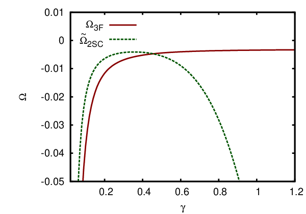
In Fig. 9 we show the results for and for our example. We see that the CFL solution is favored at low values of whereas the 2SC solution becomes favored at larger values of . This phase transition is in qualitative agreement with our findings in the NJL model when is increased, cf. Fig. 3.
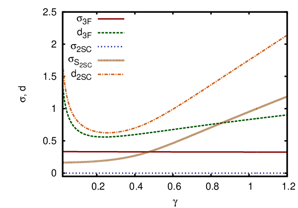
The values of the condensates associated with in minima of the free energy are shown in Fig. 10. Their behavior with rising is qualitatively similar to the effect of an increased in the NJL calculations, cf. Fig. 5. In both cases when increasing the coupling ( or ) the diquark and the strange quark chiral condensate in the 2SC phase are rising much faster than the condensates in the CFL phase.
The NJL-model results are thus completely consistent with a GL analysis if the latter is performed with a sufficiently general ansatz for the condensates.
References
- [1] P. Braun-Munzinger and J. Stachel, Nature 448, 302 (2007).
- [2] M. Cheng et al., Phys. Rev. D 81, 054510 (2010) [arXiv:0911.3450 [hep-lat]].
- [3] Y. Aoki, S. Borsanyi, S. Durr, Z. Fodor, S. D. Katz, S. Krieg and K. K. Szabo, JHEP 0906, 088 (2009) [arXiv:0903.4155 [hep-lat]].
- [4] Y. Aoki, G. Endrodi, Z. Fodor, S. D. Katz and K. K. Szabo, Nature 443, 675 (2006) [arXiv:hep-lat/0611014].
- [5] K. Rajagopal and F. Wilczek, arXiv:hep-ph/0011333.
- [6] M. G. Alford, Ann. Rev. Nucl. Part. Sci. 51, 131 (2001) [arXiv:hep-ph/0102047].
- [7] T. Schäfer, arXiv:hep-ph/0304281.
- [8] D. H. Rischke, Prog. Part. Nucl. Phys. 52, 197 (2004) [arXiv:nucl-th/0305030].
- [9] M. Buballa, Phys. Rept. 407, 205 (2005) [arXiv:hep-ph/0402234].
- [10] I. A. Shovkovy, Found. Phys. 35, 1309 (2005) [arXiv:nucl-th/0410091].
- [11] M. G. Alford, A. Schmitt, K. Rajagopal and T. Schäfer, Rev. Mod. Phys. 80, 1455 (2008) [arXiv:0709.4635 [hep-ph]].
- [12] D. T. Son, Phys. Rev. D 59, 094019 (1999) [arXiv:hep-ph/9812287].
- [13] T. Schäfer and F. Wilczek, Phys. Rev. D 60, 114033 (1999) [arXiv:hep-ph/9906512].
- [14] I. A. Shovkovy and L. C. R. Wijewardhana, Phys. Lett. B 470, 189 (1999) [arXiv:hep-ph/9910225].
- [15] T. Schäfer, Nucl. Phys. B 575, 269 (2000) [arXiv:hep-ph/9909574].
- [16] M. Asakawa and K. Yazaki, Nucl. Phys. A 504, 668 (1989).
- [17] J. Berges and K. Rajagopal, Nucl. Phys. B 538, 215 (1999) [arXiv:hep-ph/9804233].
- [18] M. A. Stephanov, K. Rajagopal and E. V. Shuryak, Phys. Rev. Lett. 81, 4816 (1998) [arXiv:hep-ph/9806219].
- [19] M. Kitazawa, T. Koide, T. Kunihiro and Y. Nemoto, Prog. Theor. Phys. 108, 929 (2002) [arXiv:hep-ph/0207255].
- [20] Z. Zhang, K. Fukushima and T. Kunihiro, Phys. Rev. D 79, 014004 (2009) [arXiv:0808.3371 [hep-ph]].
- [21] Z. Zhang and T. Kunihiro, Phys. Rev. D 80, 014015 (2009) [arXiv:0904.1062 [hep-ph]].
- [22] T. Hatsuda, M. Tachibana, N. Yamamoto and G. Baym, Phys. Rev. Lett. 97, 122001 (2006) [arXiv:hep-ph/0605018].
- [23] N. Yamamoto, M. Tachibana, T. Hatsuda and G. Baym, Phys. Rev. D 76, 074001 (2007) [arXiv:0704.2654 [hep-ph]].
- [24] G. Baym, T. Hatsuda, M. Tachibana and N. Yamamoto, J. Phys. G 35, 104021 (2008) [arXiv:0806.2706 [nucl-th]].
- [25] H. Abuki, G. Baym, T. Hatsuda and N. Yamamoto, Phys. Rev. D 81, 125010 (2010) [arXiv:1003.0408 [hep-ph]].
- [26] M. G. Alford, K. Rajagopal and F. Wilczek, Nucl. Phys. B 537, 443 (1999) [arXiv:hep-ph/9804403].
- [27] M. G. Alford, J. Berges and K. Rajagopal, Nucl. Phys. B 558, 219 (1999) [arXiv:hep-ph/9903502].
- [28] M. Buballa and M. Oertel, Nucl. Phys. A 703, 770 (2002) [arXiv:hep-ph/0109095].
- [29] M. Oertel and M. Buballa, arXiv:hep-ph/0202098.
- [30] R. Rapp, T. Schäfer, E. V. Shuryak and M. Velkovsky, Phys. Rev. Lett. 81, 53 (1998) [arXiv:hep-ph/9711396].
- [31] M. G. Alford, K. Rajagopal and F. Wilczek, Phys. Lett. B 422, 247 (1998) [arXiv:hep-ph/9711395].
- [32] S. B. Rüster, V. Werth, M. Buballa, I. A. Shovkovy and D. H. Rischke, Phys. Rev. D 72, 034004 (2005) [arXiv:hep-ph/0503184].
- [33] H. Abuki and T. Kunihiro, Nucl. Phys. A 768, 118 (2006) [arXiv:hep-ph/0509172].
- [34] H. J. Warringa, arXiv:hep-ph/0606063.
- [35] H. Basler and M. Buballa, Phys. Rev. D 81, 054033 (2010) [arXiv:0912.3411 [hep-ph]].
- [36] D. Blaschke, S. Fredriksson, H. Grigorian, A. M. Oztas and F. Sandin, Phys. Rev. D 72, 065020 (2005) [arXiv:hep-ph/0503194].
- [37] M. Kobayashi and T. Maskawa, Prog. Theor. Phys. 44, 1422 (1970).
- [38] G. ’t Hooft, Phys. Rev. D 14, 3432 (1976) [Erratum-ibid. D 18, 2199 (1978)]. G. ’t Hooft, Phys. Rept. 142, 357 (1986).
- [39] V. Dmitrasinovic, J. Math. Phys. 42, 991 (2001) [Erratum-ibid. 45, 2988 (2004)] [arXiv:hep-ph/0101008].
- [40] J. F. Nieves and P. B. Pal, Am. J. Phys. 72, 1100 (2004) [arXiv:hep-ph/0306087].
- [41] A. W. Steiner, Phys. Rev. D 72, 054024 (2005) [arXiv:hep-ph/0506238].
- [42] P. Rehberg, S. P. Klevansky and J. Hufner, Phys. Rev. C 53, 410 (1996) [arXiv:hep-ph/9506436].
- [43] M. Kitazawa, D. H. Rischke and I. A. Shovkovy, Phys. Lett. B 663, 228 (2008) [arXiv:0709.2235 [hep-ph]].
- [44] D. Nickel, Phys. Rev. Lett. 103, 072301 (2009) [arXiv:0902.1778 [hep-ph]].
- [45] D. Nickel, Phys. Rev. D 80, 074025 (2009) [arXiv:0906.5295 [hep-ph]].
- [46] S. Carignano, D. Nickel and M. Buballa, Phys. Rev. D 82, 054009 (2010) [arXiv:1007.1397 [hep-ph]].
- [47] T. Schäfer, Phys. Rev. Lett. 85, 5531 (2000). [arXiv:nucl-th/0007021].