Quantum spin nanotubes — frustration, competing orders and criticalities —
Abstract
Recent developments of theoretical studies on spin nanotubes are reviewed, especially focusing on the three-leg spin tube. In contrast to the three-leg spin ladder, the tube has a spin gap in case of the regular-triangle unit cell when the rung interaction is sufficiently large. The effective theory based on the Hubbard Hamiltonian indicates a quantum phase transition to the gapless spin liquid due to the lattice distortion to an isosceles triangle. This is also supported by the numerical diagonalization and the density matrix renormalization group analyses. Furthermore, combining analytical and numerical approaches, we reveal several novel magnetic-field-induced phenomena: Néel, dimer, chiral and/or inhomogeneous orders, new mechanism for the magnetization plateau formation, and others. The recently synthesized spin tube materials are also briefly introduced.
pacs
75.10.Jm, 75.40.Cx, 75.50.Ee, 75.50.Gg1 Introduction
The geometrically frustrated low-dimensional quantum spin systems have attracted increasing attention in recent years. Among them the spin nanotube is one of the most interesting systems, because it is expected to be a new generation of multifunctional devices. Recently some candidates for the spin nanotubes have been synthesized; three-leg tubes [(CuCl2tachH)3Cl]Cl2 [1, 2] and CsCrF4 [3], a nine-leg one [4], and a four-leg one (Refs. [5] and [6]). Several theoretical works indicated various exotic quantum phenomena of the spin tubes [10, 11, 12, 13, 14, 15, 8, 16, 9, 17, 19, 18, 20, 21, 7]. Most of them concentrated on the three-leg spin tube, because both of frustration and quantum fluctuation are the largest. In this paper, we review the recent theoretical results of the system.
In the three-leg antiferromagnetic spin tube the unit cell consists of three spins. According to the Lieb-Schultz-Mattis theorem [22], the spin gap must be accompanied with at least doubly-degenerate ground states. In fact, previous numerical analyses [11, 16, 17] have confirmed such doubly-degenerate ground states due to the spontaneous breaking of the translational symmetry along the leg direction. The ground states have a valence-bond type (dimerized) order [11, 17]. Some numerical works [16, 17, 7] indicated that the spin gap is quite fragile against the lattice distortion changing the unit cell from a regular triangle to an isosceles one. As a result, when one of the three rung couplings is changed, a quantum phase transition occurs from the spin gap to gapless phases. Developing the effective theory based on the Hubbard Hamiltonian, using the numerical exact diagonalization and the density matrix renormalization group (DMRG) approach, the ground-state phase diagram of the quantum phase transition was presented [7], reviewed in sections 3 and 4.
This system was also theoretically revealed to exhibit some exotic phenomena in magnetic field. The numerical diagonalization study [12] suggested that a magnetization plateau appears at 1/3 of the saturation for sufficiently large rung interactions. Introducing the above lattice distortion, two different plateau formation mechanisms; the up-up-down (uud) and the dimer-monomer types, are expected to appear, depending on types of isosceles triangle. Our recent work [23] has indicated a new plateau phase with a dimer and/or chiral order accompanied with the staggered moment. On the other hand, the bosonization for the weak rung-coupling regime [18] has shown that a vector chiral phase is widely present in the field-induced Tomonaga-Luttinger liquid (TLL) phase. In addition, a spin-wave type approach [19] has predicted that not only the chiral order but also an inhomogeneous magnetization order appears near the saturation. These field-induced phenomena will be discussed in detail in section 5.
The valence bond solid (VBS) ground states were revealed to appear in some different spin tube systems. For example, the quantum Monte Carlo simulation study [24] suggested that several different types of the VBS ground state occur in some chiral spin nanotubes without frustration. The recent non-linear model and DMRG approach [25] indicated some three-leg higher spin tubes exhibit several Haldane phases.
One of the most realistic candidate of the three-leg spin tube is [(CuCl2tachH)3Cl]Cl2 [2]. In this material each triangle unit cell is oriented upside-down to adjacent one, different from the straight spin tube (see section 6). The DMRG calculation of such a twisted spin tube [14, 15, 8] suggested that the material has no spin gap, which is consistent with the magnetization measurement [2].
As a future prospect, we consider the superconductivity in the carrier-doped spin nanotubes in section 7. A possible chirality induced superconductivity will be proposed as a new mechanism.
2 Isosceles spin tube
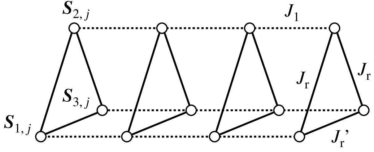
We consider the isosceles three-leg spin tube [7] shown in figure 1, described by the Hamiltonian
| (1) |
where is the spin- operator and is the length of the tube along the leg direction. The exchange interaction constant stands for the neighboring spin pairs along the legs, while and the rung interaction constants. All the exchange interactions are supposed to be antiferromagnetic (namely, positive). The ratio expresses the degree of the asymmetry of the rung interactions. Throughout this paper, we fix to unity. The effect of the magnetic field along the direction is taken into account by adding the Zeeman term to (1).
3 Effective theory
In this section, we explain low-energy effective theories for the spin tube (1). In section 3.1, we sketch a method to draw a phase diagram in the whole coupling-constant space used in [7]. Next, we investigate two special regimes and , respectively, in sections 3.1 and 3.2.
3.1 Global phase diagram derived from the Hubbard model on the tube lattice
Here, we explain a systematic method to draw global phase diagrams of one-dimensional antiferromagnetic quantum spin systems. It is well-known that Heisenberg model on an arbitrary lattice is obtained from the corresponding half-filled Hubbard model in the limit of strong on-site Coulomb interactions. Especially in one dimension, the spin configurations of the low-energy states in the Heisenberg model agree with those in the half-filled Hubbard model even with a weak Coulomb interaction [28, 26, 27]. The phase in the weak-Coulomb regime often smoothly connect to those in the strong-Coulomb regime in one-dimensional electron systems. By these arguments, we obtain a low-energy effective theory for the spin tube (1) from the corresponding Hubbard model. To discuss the wider parameter space, first we diagonalize the kinetic parts of the Hubbard Hamiltonian including both the leg and rung hopping terms [29, 30, 31]. Then, we take account of the on-site Coulomb interaction as the perturbation, with help of the Non-Abelian bosonization [32, 34, 33] and conformal field theory (CFT).
The Hamiltonian of the Hubbard model on the three-leg tube lattice
| (2) |
consists of the hopping part
and the on-site interaction part
| (3) |
where and is the repulsive coupling constant. The electron operators and satisfy the periodic boundary conditions for both the leg and the rung directions, and anticommutation relations. The hopping parameters are given by , and . The strong coupling expansion shows that this model at the half-filling case is reduced to the Heisenberg model with , and .
By a suitable unitary transformation, the hopping Hamiltonian can be written into the following diagonal form
| (4) |
where the wave number is summed over . With an orthogonal matrix , the operators and are defined by
| (5) | |||
| (6) |
which satisfy the standard anticommutation relations. The energy eigenvalues of the one-electron states are
| (7) | |||
| (8) | |||
| (9) |
Note that a degeneracy appears at due to the permutation symmetry () for .
For the half-filled case, one-electron states should be occupied by electrons with up and down spins. As a result, the ground state of the hopping Hamiltonian has one, two or three pairs of the Fermi points just on the Fermi sea, depending on the parameters and . Since the low-energy excitations are given by the particle-hole creations around these Fermi points, they can be represented by using the Dirac fermions, the left mover and the right one , which are defined from the electrons around the -th pair of Fermi points. If the -th band has no Fermi points in the half-filled case, we should neglect and . On this understanding, we approximate the original electron operators in terms of the Dirac fermions as follows:
| (10) |
where is the lattice spacing with dimension of length and is the continuous position coordinate. We add the on-site Coulomb interaction (3) to this free Dirac fermion system, and use the Non-Abelian bosonization techniques. Following the field-theory argument in [28], we expect that for the number of Fermi-point pairs is odd (even), the spin excitations are gapless (gapped) in the half-filled Hubbard tube. In particular, in the cases of one or two Fermi-point pairs, we can explicitly determine whether or not a spin gap exists as follows.
First, we consider the case of one pair of Fermi points and . In this case, the interaction (3) is approximated as the sum of a Umklapp interaction and two marginal ones
| (11) |
where are positive coupling constants proportional to . The Umklapp term is expressed as
| (12) |
and the marginal interaction between the U(1) charge currents is given by
| (13) |
where . It is known that the bosonized form of contain only the charge degrees of freedom and they open a charge gap when is positive. Then, the remaining spin degrees of freedom are described by the gapless level-1 SU(2) Wess-Zumino-Witten (WZW) theory [32, 34, 33]. This phenomenon, i.e., the charge-spin separation is well-known in the single Hubbard chain model. For this WZW theory, the third interaction
| (14) |
is known to be marginally irrelevant if . Except the above interactions , there is no relevant operator with the invariance under the one-site translation along the leg,
| (15) |
as in the case of the Heisenberg chain. The spin excitations remain gapless.
On the other hand, when there exist two pairs of the Fermi points, and , the spin excitations are suffered from relevant interactions. In this case, the spin sector in the hopping part of the Hubbard tube is described by a level-2 SU(2) WZW model derived from two decoupled Dirac fermions [38]. The Coulomb interaction yields several perturbations for this theory. For example, the following term
| (16) |
contains a relevant perturbation in the level-2 WZW model, which is invariant under the translation
| (17) |
Particularly for , much more relevant operators are allowed by the translational invariance because of the coincident Fermi points and . Therefore, we conclude that any gapless spin excitation generally has no chance to survive except particularly rare cases [e.g., when the coupling constant of (16) is zero].

For the case of three Fermi-point pairs, the interactions among three Dirac fermions are generated from (3), and thus it is difficult to analyze them and judge whether or not the spin excitation can survive as gapless. The gapless spin excitation is expected from [28, 35].
From these arguments, we can draw the ground-state phase diagram of the half-filled Hubbard tube shown in figure 2. The phase (I) has three pairs of the Fermi points, the phases (II) and (IV) have one pair, and the central phase (III) has two pairs. Therefore, we predict that the phases (II) and (IV) have gapless spin excitations, whereas the phase (III) possesses a spin gap. By and obtained from strong on-site interaction, figure 2 depicts the phase diagram of the three-leg spin tube (1). Since we have treated the on-site interaction perturbatively in the effective theory, we should not trust the obtained phase boundaries as accurate ones. Note that the gapful phase (III) is predicted to be extended around the line for a finite . In the limit , the both the left- and right-side phase boundaries of the region (III) converge to . This narrowing of the phase (III) is consistent with the numerical results [16, 17] in the strong-rung-coupling limit .
Finally, we argue the universality classes of the phase transitions at two phase boundaries, (II)-(III) and (III)-(IV). For the level-1 SU(2) WZW model in the phases (II) and (IV), the most relevant perturbation is the marginal current-current interaction [32, 34, 33], (14), which is the only allowed invariant interaction. Since it can be marginally “relevant” when parameters are finely tuned and then becomes negative, we speculate that the transition from the phases (II) or (IV) to (III) is caused by this marginal term. Therefore, the transitions are expected to be in the Berezinskii-Kosterlitz-Thouless (BKT) universality class [36, 37].
3.2 Gapless phase for
In section 3.1, we have obtained a qualitative phase diagram of the spin tube (1) as shown in figure 2. However, some subtle points still remains. Particularly the existence of the gapless phase (I) should be discussed. Here, we focus on the right-lower regime in figure 2 . In this regime, we discuss the existence of the gapless phase (I) and the phase transition between the gapless phase (I) and the gapful phase (III).
We introduce three level-1 SU(2) WZW models for the three decoupled Heisenberg chains [32, 34, 33], and we treat their rung couplings as the perturbation The first and the third chains are coupled to each other with which is much stronger than two remaining couplings . It is well-known that the coupling involves a relevant interaction with conformal dimensions in the two coupled WZW models, it produces an energy gap [39]. This relevant operator behaves like the mass operator in the corresponding effective field theory. On the other hand, like the case of one Fermi-point pair in section 3.1, the WZW model for the second chain has the marginal irrelevant interaction with a finite negative coupling constant . The operator is equivalent to (14), if we use the Dirac fermions to describe the second chain. The negative sign makes irrelevant and the second chain is gapless. A weak rung coupling between this WZW model and the massive theory for the two coupled chains must give a correction to the coupling constant . If is sufficiently small, the sign of would not change and the gapless excitation is preserved. These arguments convince us that the gapless phase (I) definitely exists. Furthermore, we expect the phase transition from the gapless phase (I) to the gapful phase (III). Namely, if exceeds a critical value, the coupling constant might change to be positive. In this case, the operator becomes marginally relevant, which produces an excitation gap. Since the operator is marginal, this transition between the phases (I) and (III) is of the BKT type [36, 37], as in the zigzag Heisenberg chain [40]. The effective theory for is obtained, and the transition from the phase (I) to (III) is discussed in [7].
3.3 Perturbation theory from the strong rung coupling limit
In case of , the perturbation theory from the independent triangle limit will work well. Let us begin with the case (i.e., three-spin problem), which can be easily solved and there are 8 eingenstates. Here represents the wave function with eigenvalues , and , where is the eigenvalue of the rung-parity operation . The state is abbreviated as for example and denotes the singlet pair . We show four eigenstates with only, because other four eigenstates with can be easily obtained by interchanging ;
| (18) |
These wave functions do not depend on because all of them are completely classified by the eigenvalues , and . The lowest energy states are for , while they are for .
The first order perturbation theory with respect to , retaining four states with having lower energies and neglecting other 4 states with leads to
| (19) |
where is a spin-1/2 operator acting on and is also a spin-1/2 operator acting as
| (20) |
where indices were omitted for simplicity. The energy difference between and acts as a “magnetic field” applied on spins. This is essentially the same as that obtained by Nishimoto and Arikawa [17].
In case of sufficiently strong asymmetry , the spins are completely polarized and only spins survive, where is reduced to that of the antiferromagnetic Heisenberg chain having the gapless excitation. Thus the phase (III) has a finite width along the line . Next, let us focus on the region around the symmetric line . In the limit , the ground state has saturated spins at any asymmetric point . For a finite , however, we expect an extended gapful phase around , if the energy gap exists at due to the coupling between and spins. The finite energy gap does not vanish by an infinitesimal external field . In other words, the magnetization process of the spins should show a zero-magnetization plateau. Therefore, an energy gap would also be present for sufficiently weak asymmetry .
For the rest of this subsection we suppose (i.e. regular triangle case) where the translational invariance by one site along the rung direction holds and the lowest energy states are 4-fold degenerate. In this case another set of useful expressions for the lowest energy states is
| (21a) | |||||
| (21b) | |||||
| (21c) | |||||
| (21d) | |||||
where and indices and denote the wave number and along the rung direction, respectively. The first order perturbation theory with respect to , retaining above four states with and neglecting other 4 states with leads to [10, 11]
| (21v) |
where is a spin-1/2 operator acting on the first indices of the above states and are the spin-1/2 matrices acting on the second indices as
| (21w) |
Of course this can be obtained from (19) through the unitary transformation and letting .
Schulz [10] analyzed using the Jordan-Wigner transformation and concluded that the system is gapped. Kawano and Takahashi [11] performed the DMRG calculation for to find that Hamiltonian has a spin gap of . When the next-nearest-coupling term having a special coupling constant is added to (21v) they found the exact ground state closely similar to the Majumdar-Ghosh state, which is spontaneously dimerized and breaks the translational symmetry. They insisted that the ground state of (21v) is similar to this Majumdar-Ghosh state, and provided strong numerical evidences.
4 Spin gap and ground-state phase diagram — numerical study
In this section the numerical ground state phase diagram of the isosceles spin tube obtained in our previous work[7] is presented. The method to derive it is the phenomenological renormalization combined with the numerical diagonalization up to and the DMRG up to .
A useful order parameter to determine the phase boundaries between the gapless and the gapful phases is the spin gap , which is the energy gap between the singlet ground state and the triplet excited state in the finite, but large system. We calculate it by means of the DMRG up to .
In order to determine a phase boundary of the usual second order phase transition, the phenomenological renormalization equation is often used effectively. For the present critical point , however, this type of phenomenological renormalization has no clear crossing point, but the scaled gap increases with increasing in both gapless and gapful phases. This is because the scaled gap is an increasing function with respect to not only in the gapful phase but also in the gapless phase, since the finite-size gap must have the logarithmic size correction term . Here, we should recall that the logarithmic correction normally vanishes just at due to the SU(2) symmetry in the CFT [40]. Therefore, instead of using the crossing point of the scaled gaps, we can estimate as a point where the size correction is minimized. Note that the minimum value decreases as the size increases. This phenomenon and the assumption of the BKT type transition suggest that this minimal value approaches zero as the system size increases. This is quite reasonable if we suppose the most important finite-size correction to the scaled gap next to term is order of [40, 41, 42]. We thus determine from the minimums for two large systems with and for . The estimated and are shown as crosses in figure 3. They correspond to the phase boundary between two regions (II) and (III) and that between (III) and (IV), respectively. At least these boundaries for the strong-rung-coupling regime are precise enough to justify that a finite gapful phase (III) exists. However, it is difficult to obtain for , because the DMRG calculation does not well converged there.
In order to determine the phase boundaries for the weak-rung-coupling regime , we use the minimum points of calculated by the numerical diagonalization up to under the periodic boundary condition. Using the estimated phase boundaries for and (8,10), and assuming the size correction is proportional to in both directions of and the phase boundaries among the phases (I), (II), (III) and (IV) in the thermodynamic limit were estimated. The phase boundaries are also shown as solid curves in figure 3. At least the phase boundaries (II)-(III) and (III)-(IV) are consistent with the DMRG results for . The boundary (III)-(IV) is, however, significantly deviated from the DMRG estimation for . This discrepancy is supposed to be due to the error of extrapolation. This analysis also justifies the existence of the phase (I). However, the error of extrapolation becomes larger as we approach the line in the case of . Thus it is difficult to conclude that the phase (I) really exists for within the present numerical demonstration. It is also difficult to confirm the boundary (I)-(II), and the phase (I) might combine with the phase (II) in a certain regime with .

The phase boundaries between the phases (I) and (III), as well as (III) and (II), for smaller (), were well reproduced by the level spectroscopy method [40, 43, 44, 45], which is one of precise techniques to estimate the critical point for the BKT transition. But the level spectroscopy method does not work well for larger , because of too large finite-size corrections.
5 Field-induced phenomena
In this section, we consider effects of applied magnetic field in three-leg spin tubes. Particularly, we focus on field-induced phases (vector chiral order and magnetization plateau) and quantum phase transitions.
5.1 Vector chiral phase in the weak rung-coupling regime
Here, we study the weak rung-coupling regime in a magnetic field [18], namely, the Hamiltonian,
| (21x) |
with . If a sufficiently strong magnetic field is applied and a finite magnetization occurs, the spin-rotational SU(2) symmetry is reduced to the U(1) type, in which the Abelian bosonization [33, 34, 52] becomes reliable at least for the weak rung-coupling regime. At the zero rung-coupling limit, the low-energy properties of -th spin chain in the tube can be described by a free boson theory whose Hamiltonian is given by
| (21y) |
Here, and are the pair of dual scalar fields (), and and respectively denote the TLL parameter and the excitation velocity. The spin operator is also bosonized as
| (21z) |
with and being nonuniversal constants. Here, is the magnetization per site. In the present notation, runs from 1/2 to 1 when the magnetization is increased from 0 to the saturated value 1/2. Using the formula (21z), we can obtain the bosonized form of the perturbative rung coupling, and the resultant effective Hamiltonian for the spin tube is expressed as
| (21aa) | |||||
Here we have neglected all the terms with oscillating factors or , and have introduced new pairs of boson fields; , , and . The first line in (21aa) is equivalent to three copies of TLLs in decoupled chains. The second line is linear terms which induce just a small correction to the magnetization . In the isosceles case , would be realized. The third and fourth lines are quadratic terms changing the values of and . In the regular-triangle case, the quadratic part is diagonalized in the basis of , and resultant TLL parameters and velocities for sectors, and , are calculated as , , and . The fifth and sixth lines correspond to the vertex-type perturbations, and the function is defined by
| (21ab) |
In our notation, the scaling dimension of vertex operators are given as and at the decoupled case. We should emphasize that (21aa) does not include any relevant terms with and except for commensurate cases with ( and : integer). This property is protected by spin-rotational and translational symmetries of the spin tube. Therefore, the sector is described by a TLL. On the other hand, the remaining sectors are subject to the vertex terms.
We first focus on the regular-triangle case analyzing the above effective Hamiltonian (21aa). In this case, two vertex perturbations and in (21aa) vanish, and the scaling dimensions of and are readily evaluated: and . In the weak rung-coupling regime, is very close to and holds in the magnetization process. Therefore, is more relevant and sectors have gapped spectra. The form of the potential is shown in figure 4(a), in which the diamond region is meaningful in the full - plane and it is called here physically relevant zone. Remarkably there are two minimum points in the diamond zone: .

A minimum is mapped to the other via sign change that can be realized by the exchange of two chains and . This suggests a spontaneous breakdown of rung-parity symmetry. Vector chiralities in rung bond is a natural candidate for the order parameter, and the bosonized forms of their components are given as
| (21ac) |
At the point (), becomes positive (negative). From the translational symmetry along the rung, we can predict . We thus conclude that in the weak rung-coupling regime with and a finite , the low-energy physics is governed by the TLL in the sector and the remaining gapped sectors generate a vector chiral long-range order with spontaneously breaking the rung-parity symmetry. In the commensurate case of , there appears the magnetization plateau at least in a strong rung-coupling regime (see the next subsection). It has been predicted in [12] that the plateau survives up to a fairly weak rung-coupling regime () at the regular-triangle case . From the bosonization viewpoint, the plateau is attributed to the emergence of a spin gap of sector induced by a higher-order perturbation . In fact, this vertex term may be relevant at in which the factor is equal to unity. This corresponds to so-called gapped chiral phase; the system has a gapped spectrum and a vector chirality is long-range ordered. In other words, the spin tube offers a unique chance to observe both gapless and gapped vector-chiral phases in the magnetization process.
Next we consider effects of the rung deformation, . Even in this isosceles case, the chirality between the first and third chains is still useful as a order parameter because the tube is invariant under rung parity operation between these two chains. Due to the rung deformation, all kinds of the rung coupling terms in (21aa) are modified. As already mentioned, the boson linear terms just slightly change the uniform magnetization . The quadratic term cannot be diagonalized in the present basis, but its effects would be quite small and the qualitative nature of the vector chiral phase is expected not to be changed. The most important point of the rung deformation is the change of the vertex potential due to an additional term in the fifth line of (21aa). The modified potential is expressed as follows:
| (21ad) | |||||
Figure 4(b) presents this potential as a function of with fixing . It clearly shows that the potential form is changed from a double-well type to a single-well type for , while the form is always double-well type for . This classical argument predicts the critical point , and the chiral order is expected to disappear in . To gain deeper understanding of this expectation, we consider the effective theory for sector. If we naively replace with its mean value in the potential , the effective Hamiltonian is obtained as
| (21ae) | |||||
This is nothing but a double-frequency sine-Gordon model. Under the condition , this model is believed to exhibit an Ising-type quantum phase transition by tuning the ratio of two coupling constants [53, 54]. We can hence predict the phase diagram of the isosceles spin tube with a weak rung coupling and a finite magnetization as shown in figure 5.

The chiral ordering occurs in the region . The true critical value must deviate from its classical one . The order parameter behaves as near the transition point. From this figure, one also finds that once a coupling between a two-leg ladder and a single chain is introduced, a vector chiral order immediately emerges.
Similar scenarios of a vector chiral order and an Ising transition are also expected in other tubes consisting of spin chains with a TLL parameter . For instance, even in the zero-field case, spin tubes with easy-plane XXZ anisotropy must yield a chiral order in the weak rung-coupling regime. It is known that the field-induced TLL phase satisfies in a spin-1 antiferromagnetic Heisenberg chain [55] and the leading term of bosonized spin operator has the same form as that of (21z) [56, 57]. Therefore, three-leg spin-1 tubes have a vector chiral order at least in high-field and weak rung-coupling regime. In the vicinity of the saturation field, three-leg spin- tubes can be analyzed by spin-wave type approach [19]. It also predicts the emergence of the vector chiral order in a certain weak rung-coupling regime. These results obviously suggest that a vector chiral order is generally induced by applied magnetic field in three-leg spin- antiferromagnetic tubes with a weak rung coupling. The spin-wave approach also points out the possibility of an inhomogeneous magnetization phase with [19] in the regular-triangle case.
5.2 1/3 plateau
The magnetization plateau at surely exists for since the triangle unit cell is composed of three spins, while it does not exist for the because the system is reduced to three independent spin chains in this limit. Thus the plateau phase diagram on the plane is of immense interest.
As discussed in section 3.1, we study magnetization plateaux in the effective Hubbard model under external field. The Zeeman term for electrons is given by
| (21af) |
which should be added to the Hubbard Hamiltonian. Elaborated analysis of the effective theory for this Hubbard model gives the conditions for the existence of the spin excitation gap. Then, we show the existence of the 1/3 magnetization plateau and nonexistence of any other nonzero magnetization plateaux. Details will published elsewhere [58]. The phase diagram of the 1/3 magnetization plateau is depicted in figure 6. This agrees with the numerical calculation qualitatively, as shown later.

Let us discuss the 1/3 plateau problem by use of the effective Hamiltonian (19) supposing . In the 1/3 plateau case we can fix and retain the degree of freedom with respect to , resulting in
| (21ag) |
In other words, we take only two states in (18) into consideration. We note that describes states only, because both of have corresponding to .
is nothing but the chain in transverse magnetic field, which is a special case of the chain in transverse magnetic field of which ground state was investigated by Dmitriev et al [59, 60, 61], and Capraro and Gros [62]. Their results can read as follows in our cases. Both of and have the long-range order for the weak “magnetic field” case (i. e. ), while only has the long-range order for the strong “magnetic field” case (i. e. ). The boundary between above two cases will be approximately given by . In the latter case the state of the unit triangle is essentially either or according as or . In the former case, on the other hand, there exists the long-range Néel order of spins along the direction associated with the spontaneous breaking of the translational symmetry (SBTS) and the two-fold degeneracy of the ground state. In this case the ground state energy (the energy of the state in the original spin language) will be considerably lowered by the interaction effects, which leads to the remarkable increase of the width of plateau. Further the SBTS of the system results in the SBTS and the spontaneous breaking of the inversion symmetry of in the original spin representation. If we suppose the complete Néel order of along the direction , for simplicity (this situation will be a good approximation of the ground state in case of extremely weak “magnetic field” ), the expectation values of are
| (21ah) |
which shows the spontaneous breaking of the translational symmetry () and inversion symmetry ().
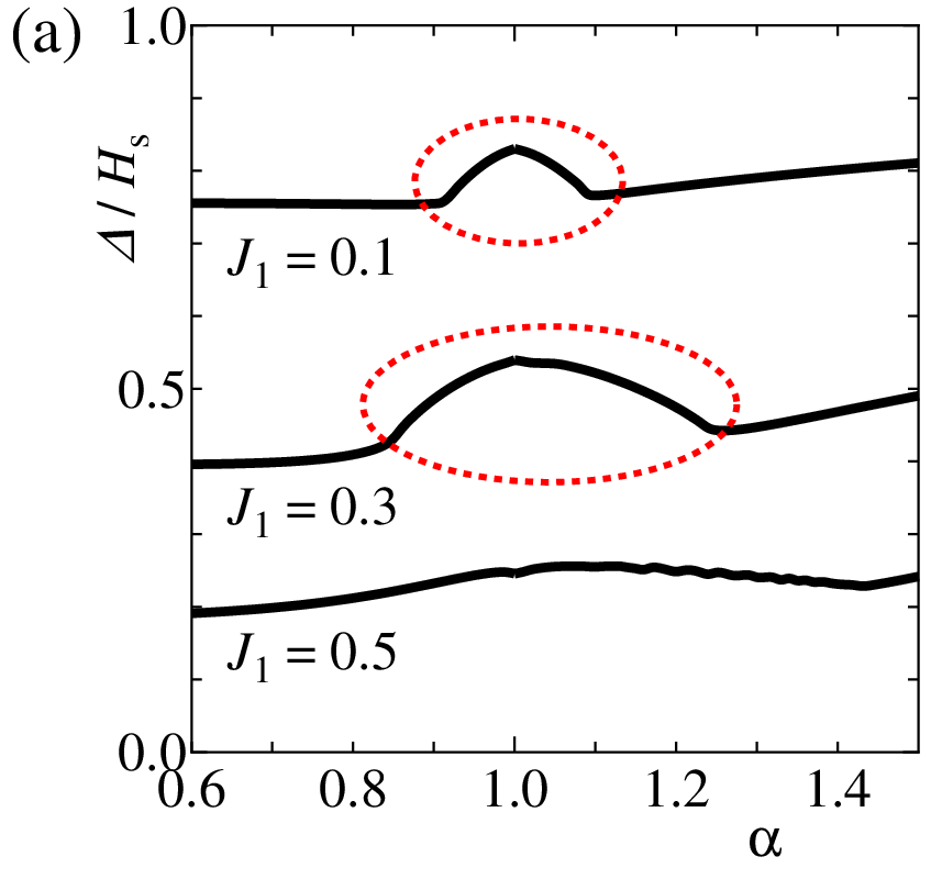

Figure 7(a) shows the dependence of the magnetization plateau width , from which we can see the anomalous increase of the near at least for and 0.3 cases as predicted by the above theoretical consideration. In usual cases the plateau width (or the spin gap) is remarkably decreases near the mechanism-changing point and often becomes zero at that point, as shown in figure 7(b). Thus, we find a new and exotic behavior of the plateau width, which is completely opposite to that of usual cases [63]. In the case, for instance, the plateau is realized by the and mechanisms for and , respectively, while by the cooperative effects of both mechanisms for . We note that the excitation gap (i. e., magnetization plateau width) from the state to states is always finite when is varied. When and , the expectation values obtained by DMRG are
| (21ai) |
which well agree with the theoretically predicted values in (21ah). Details will be published elsewhere [58].
Let us explain why the new and exotic behavior of the plateau width is realized in our model, by comparing our model with the bond-alternating Heisenberg chain described by
| (21aj) |
where is the bond alternation parameter. Any small amount of produces the dimer spin gap as [64, 65, 66] (with leading logarithmic correction [67]). Thus the spin gap of (21aj) behaves as the sketch in figure 7(b) near . When (), the spins and ( and ) effectively form a singlet dimer pair, which brings about the dimer spin gap. These two mechanism, and mechanisms, are completely competing and the reconstruction of the unit cell occurs at the mechanism changing point . At the system is of the Tomonaga-Luttinger state which is characterized by the gapless excitation. In our case, on the other hand, the unit cell is always the isosceles triangle for both of and cases. Then the reconstruction of the unit cell never occur in our case, which enables the cooperation of two plateau-formation mechanisms, mechanism and mechanism.

The phase boundary between the traditional plateau phases and the new plateau phase where the plateau width remarkably increases can be determined by the phenomenological renormalization equation for the scaled gap obtained by the numerically exact diagonalization method
| (21ak) |
where is the excitation gap within the space and is the size-dependent fixed point of . The plateau-plateauless phase boundary can be estimated also by the phenomenological renormalization equation where is replaced by (plateau width) as in case of the spin gap at . Figure 8 shows our preliminary results on the phase diagram at . This phase diagram qualitatively agrees with figure 6. However more detailed analyses will be necessary to draw a precise phase diagram.
6 Twisted tube
Although we have discussed theoretical aspects of the isosceles quantum spin tube, a compound corresponding to our model has not been found yet. In this section, we review the twisted spin tube, which is of particular importance for actual experiments; Recently, the interesting compound [(CuCl2tachH)3Cl]Cl2 was actually synthesized as an assembly of the triangular cluster conformed by Cu++ ions and magnetization measurements were performed [2]. As is in figure 9, the tube structure of this compound is based on the alternatingly-aligned triangles, where the exchange coupling in the unit triangle is denoted as and the intra-triangle coupling is written as . The low-energy properties of the quantum spin tube were theoretically studied by DMRG [15, 14]. Also, the quantum spin tube with the easy-plane anisotropy was investigated in the context of the triangular lattice spin system and then interesting field induced phase transitions were observed in the magnetization curve [68].
At the early stage of study, [(CuCl2tachH)3Cl]Cl2 might have a small spin gap, based on the susceptibility measurement above 2K. However, the succeeding studies have clarified that the observed spin-gap-like behavior around K crossovers to the gapless behavior at very low temperature region (K) [69], which is consistent with the theoretical results. This suggests that a kind of dual structure associated with the quantum phase transition of the first order may be captured by the experimental measurements. Below, we will review the quantum phase transition peculiar to the twisted quantum spin tube.

The model Hamiltonian of the twisted spin tube is written as,
| (21al) |
with the periodic boundary condition in the -direction. A naive consideration about the lattice structure of this twisted tube suggests that a quantum phase transition between the following two phases may occur; For , the system is described by the almost decoupled triangles, where the chirality degree of freedom defined on the unit triangle plays crucial role, while for , the lattice structure is basically described as a rhombus lattice. Note that, if , the rhombus lattice has no frustration. Thus we can expect a quantum phase transition between decoupled-triangles and rhombus lattice phases.
In the decoupled triangle limit(), the degenerate perturbation with respect to leads us to the effective spin-chirality model,
| (21am) |
where represents the spin operator and indicates an effective spin matrix representing the chirality degrees of freedom as in (21v). This effective Hamiltonian is very similar to (21v); The phase factor originates from the rotation of the lattice along the tube direction and it can be removed by the gauge transformation. On the same line of the argument as (21v), the effective Hamiltonian (21am) has a spin gap[10, 11, 13]. Indeed, a detailed DMRG computation of the full Hamiltonian (21al) actually confirms that the spin gap exists for [15, 14]. For , on the other hand, the finite size scaling analysis of the spin gap basically indicates the gapless ground state [15]. Although the usual singlet-triplet spin gap for the open boundary condition captures a boundary excitation in , such an anomalous behavior due to the boundary can be settled down by using the single-spin termination of the tube [8].
In order to resolve nature of the quantum phase transition of the twisted tube, an important quantity is the total- on the unit triangle [14]. For decoupled triangle, the ground state is in doubly degenerating doublets of the unit triangle, while for , the ground state basically belongs to sector. Here, we define the projection operator of the total- of the unit triangle to the doublet sector as for each unit triangle. As discussed in [14], then, this projection operator is a good order parameter of the twisted tube; The detailed computation of the expectation value shows discontinuity at the critical value not at , which is consistent with the spin gap result. In addition to this, we should remark that an extended spin tube with the diagonal interaction shows the exact first order phase transition, for which total- on the unit triangles independently conserves [70]. We have thus investigated how to connect the twisted tube to the diagonal interaction model. We add
| (21an) |
to the Hamiltonian (21al), and then varies . Note that corresponds to the original twisted tube and does to the diagonal spin tube, which shows the first order transition at [70].

In figure 10, we show at the center of the extended tube calculated by DMRG for with . In the figure, jumps exactly from zero to unity at along the line of , where the total- of the unit triangle is the exact symmetry. Then, we can see that the “gap” of the is adiabatically continued to . This implies that the transition at on the line of corresponding the twisted tube (21al) is of first order. As increases in , this gap reduces, but we can not confirm whether the end point of the first order transition exist or not within the present calculations for . However, we think that the overview of the first order quantum phase transition is clarified.
In connection with the experiments, an interesting point is that the parameter for [(CuCl2tachH)3Cl]Cl2 is located in the gapless sector, but it is surrounded by the “gap” of the first-order transition, as in figure 10. This implies that, although the ground state itself is gapless, a certain density of states originating from the sector can be expected above the ground state. Thus we can expect that such dual structure of and 3/2 sectors affects the experimentally observed quantities of the twisted tube at a finite temperature. Indeed, a recent specific heat result illustrates that the linear temperature dependence at very low temperature(K), which can be described as an effective chain, crossovers to spin-gap-like increasing around K [69]. Also for the low-field magnetization curve of , we can see that, after linear increase of the magnetization at very low field region, the slope of the magnetization curve rapidly increases, as if it had a spin gap [15].
7 Future prospects
As a future prospect, it would be interesting to consider the carrier-doped spin nanotube like the high-Tc cuprates, where the system is effectively described by the Hubbard model near the half-filling case. A mechanism of the superconductivity based on the spin gap had been proposed for the carrier-doped two-leg spin ladder [71] and actually a pressure-induced superconductivity was observed on the spin ladder cuprate [72]. Motivated by the discovery, the spin gap mediated superconductivity was theoretically proposed even for the three-leg spin ladder, using the quantum Monte Carlo simulation [73, 74]. If the carrier-doped three-leg spin tube is realized, it would be a better candidate of the superconductor, rather than the three-leg ladder, because it has a spin gap. In addition the three-leg spin tube was also revealed to have an energy gap in the chirality degrees of freedom [13]. It suggests that a chirality induced superconductivity would be possibly realized as a new mechanism of superconductivity in the near future.
References
References
- [1] Seeber G, Kögerler P, Kariuki B M and Cronin L, Chem. Commun. (2004) 1580
- [2] Schnack J, Nojiri H, Kögerler P, Cooper G J T and Cronin L 2004 Phys. Rev.B 70 174420
- [3] Manaka H, Hirai Y, Hachigo Y, Mitsunaga M, Ito M and Terada N 2009 J. Phys. Soc. Jpn. 78 093701
- [4] Millet P, Henry J Y, Mila F and Galy J 1999 J. Solid State Chem. 147 676
- [5] Garlea V O, Zheludev A, Regnault L -P, Chung J -H, Qiu Y, Boehm M, Habicht K and Meissner M 2008 Phys. Rev. Lett. 100 037206
- [6] Garlea V O, Zheludev A, Habicht K, Meissner M, Grenier B, Regnault L -P and Ressouche E 2008 arXiv:0807.1571.
- [7] Sakai T, Sato M, Okunishi K, Otsuka Y, Okamoto K and Itoi C 2008 Phys. Rev.B 78 184415
- [8] Okunishi K, Yoshikawa S, Sakai T and Miyashita S 2009 Int. J. Mod. Phys. C 20 1423
- [9] Sakai T, Okunishi K, Okamoto K, Sato M, Matsumoto M and Otsuka Y 2007 J. Magn. Magn. Mater. 310 e423
- [10] Schulz H J 1996 in Correlated Fermions and Transport in Mesoscopic Systems, ed. Martin T, Montambaux G, Tran Than Van J (cond-mat/9605075)
- [11] Kawano K and Takahashi M 1997 J. Phys. Soc. Jpn. 66 4001
- [12] Cabra D C, Honecker A and Pujol P 1998 Phys. Rev.B 58 6241
- [13] Luscher A, Noack R M, Misguich G, Kotov V N and Mila F 2004 Phys. Rev.B 70 060405(R)
- [14] Fouet J -B, Läuchli A, Pilgram A, Noak R M and Mila F 2006, Phys. Rev.B 73 014409
- [15] Okunishi K, Yoshikawa S, Sakai T and Miyashita S 2005 Prog. Theor. Phys. Suppl. 159 297
- [16] Sakai T, Matsumoto M, Okunishi K, Okamoto K and Sato M 2005 Physica E 29 633
- [17] Nishimoto S and Arikawa M 2008 Phys. Rev.B 78 054421
- [18] Sato M 2007 Phys. Rev.B 75 174407
- [19] Sato M and Sakai T 2007 Phys. Rev.B 75 014411
- [20] Sato M 2005 Phys. Rev.B 72 104438
- [21] Sato M and Oshikawa M 2007 Phys. Rev.B 75 014404
- [22] Lieb E, Schultz T and Mattis D 1961 Ann. Phys. 16 407
- [23] Sakai T, Okunishi K, Okamoto K, Itoi C and Sato M 2010 J. Low Temp. Phys. 159 55
- [24] Matsumoto M, Sakai T, Sato M, Takayama H and Todo S 2005 Physica E 29 660
- [25] Charrier D, Caopponi S, Oshikawa M and Pujol P 2010 cond-mat/1005.0711.
- [26] Affleck I, Nucl. Phys. B 265 (1986) 409
- [27] Ledermann U, Le Hur K and Rice T M, Phys. Rev. B 62 (2000) 16383
- [28] Affleck I and Haldane F D 1987 Phys. Rev.B 36 5291
- [29] Balents L and Fisher M P 1996 Phys. Rev.B 53 12133
- [30] Arrigoni E 1996 Phys. Lett. A 215 91
- [31] Lin H, Balents L and Fisher M P 1997 Phys. Rev.B 56 6569
- [32] Affleck I 1989 in Fields, Strings and Critical Phenomena, 1988 Les Houches Lecture Notes, edited by E. Brézin and J. Zinn-Justin (Elsevier, Amsterdam) p 564.
- [33] Gogolin A O, Nersesyan A A and Tsvelik A M 1998 Bosonization and Strongly Correlated Systems (Cambridge University Press, UK)
- [34] Tsvelik A M 2003 Quantum Field Theory in Condensed Matter Physics, 2nd edition (Cambridge University Press, UK)
- [35] Totsuka K and Suzuki M 1996 J. Phys. A: Math. Gen.29 3559
- [36] Berezinskii Z L 1970 Zh. Eksp. Teor. Fiz. 59 907 (Sov. Phys.-JETP 1971 32 493)
- [37] Kosterlitz J M and Thouless D J 1973 J. Phys. C: Solid State Phys.6 1181
- [38] We have neglected the difference between the Fermi velocities of the first and second bands.
- [39] Shelton D G, Nersesyan A A and Tsvelik A M 1996 Phys. Rev.B 53 8521
- [40] Okamoto K and Nomura K 1992 Phys. Lett. A 169 433
- [41] Cardy J L 1986 J. Phys. A: Math. Gen.19 L1093
- [42] Cardy J L 1987 J. Phys. A: Math. Gen.20 5039
- [43] Nomura K and K. Okamoto K 1994 J. Phys. A: Math. Gen.27 5773
- [44] Okamoto K 2002 Prog. Theor. Phys, Suppl. No. 145 113
- [45] Nomura K and Kitazawa A 2002 Proc. French-Japanese Symp. on Quantum Properties of Low-Dimensional Antiferromagnets ed Y. Ajiro and J-P. Bouhcer (Kyushuu University Press, Fukuoka, Japan) (cond-mat/020172)
- [46] Cardy J L 1984 J. Phys. A: Math. Gen.17 L385
- [47] Blöte H W, Cardy J L and Nightingale M P 1986 Phys. Rev. Lett. 56 742
- [48] Affleck I 1986 Phys. Rev. Lett. 56 746
- [49] Itoi C and Kato M -H 1997 Phys. Rev.B 55 8295
- [50] Giamarchi T and Schulz H J 1989 Phys. Rev.B 39 4620
- [51] Ziman T and Schulz H J 1987 Phys. Rev. Lett. 59 140
- [52] Giamarchi T 2004 Quantum Physics in One Dimension (Oxford University Press)
- [53] Fabrizio M, Gogolin A O and Nersesyan A A 2000 Nucl. Phys.B580 647
- [54] Bajnok Z, Palla L , Takács G, and Wágner F 2001 Nucl. Phys.B601 503
- [55] Fáth G 2003 Phys. Rev.B 68 134445
- [56] Essler F H L and Affleck I 2004 J. Stat. Mech.: Theor. Exp. P12006
- [57] Sato M 2006 J. Stat. Mech.: Theor. Exp. P09001
- [58] Okamoto K, Sakai T, Sato M, Okunishi K and Itoi C, in preparation
- [59] Dmitriev D V, Krivnov V Ya and Ovchinnikov 2002 Phys. Rev.B 65, 172409
- [60] Dmitriev D V, Krivnov V Ya, Ovchinnikov and Langari A 2002 J. Exp. Theor. Phys. 95 538 (Zh. Eksp. Teor. Fiz. 122 624)
- [61] Dmitriev D V and Krivnov 2004 Phys. Rev.B 70 144414
- [62] Capraro F and Gros C 2002 Eur. Phys. J. B 29 35
- [63] Okamoto K, Sato M, Okunishi K, Sakai T and Itoi C 2010 Physica E to appear
- [64] Cross M and Fisher D S 1979 Phys. Rev.B 19 402
- [65] Nakano T and Fukuyama H 1980 J. Phys. Soc. Jpn. 49 1679
- [66] Okamoto K, Nishimori H and Taguchi Y 1986 J. Phys. Soc. Jpn. 55 1458
- [67] Black J L and Emery V J 1981 Phys. Rev.B 23 429
- [68] Yoshikawa S, Okunishi K, Senda M and Miyashita S 2004 J. Phys. Soc. Jpn. 73 1798
- [69] Ivanov N B, Schnack J, Schnalle R, Richter J, Kögerler P, Newton G N, Cronin G, Oshima Y and Nojiri H, Phys. Rev. Lett. 105 (2010) 037206
- [70] Honecker A, Mila F and Troyer M 2000, Eur. Phys. J. B 15 227
- [71] Rice M, Gopalan S and Sigrist M 1993 Europhys. Lett. 23 445
- [72] Uehara M, Nagata T, Akimitsu J, Takahashi H, Môri N and Kinoshita K 1996 J. Phys. Soc. Jpn. 65 2764
- [73] Kimura T, Kuroki K and Aoki H 1996 Phys. Rev.B 54 R9608
- [74] Kimura T, Kuroki K and Aoki H 1998 J. Phys. Soc. Jpn. 67 1377