Percolation Approach to Study Connectivity in Living Neural Networks
Abstract
We study neural connectivity in cultures of rat hippocampal neurons. We measure the neurons’ response to an electric stimulation for gradual lower connectivity, and characterize the size of the giant cluster in the network. The connectivity undergoes a percolation transition described by the critical exponent . We use a theoretic approach based on bond–percolation on a graph to describe the process of disintegration of the network and extract its statistical properties. Together with numerical simulations we show that the connectivity in the neural culture is local, characterized by a gaussian degree distribution and not a power law one.
Keywords:
neural networks, graphs, connectivity, percolation, giant componentClassification:
87.18.Sn, 87.19.La, 64.60.Ak1 Introduction
Neurons in living networks form a highly rich web of connections in which activity flows between neurons through synapses. The most fascinating living neural network is the human brain, but its complex architecture, functionality, and computation capability is still far from being fully understood. More impressive is that the 100 billion neurons are not randomly connected, but rather form elaborate circuits with specific tasks. Connectivity thus appears as the fundamental feature to understand the potential of a living neural network.
Unravelling the detailed connectivity diagram of a living neural network is a painstaking process. For a brain, a small section of it, or even for a small neural culture, with neurons and connections in just 1 mm2, this task is, at present, unfeasible. In the brain, substantial progress has been attained in the description of the connectivity in the mammalian cortex [1, 2], or the analysis of brain functional networks [3, 4]. However, only in the small invertebrate C. elegans [5] it has been possible to map out, in a Herculean project, the connectivity of its 302 neurons. It is not surprising then that other approaches, different than the pure physiological ones, are being introduced to extract information about the connectivity of neural networks or, at least, some relevant statistical properties.
Biological neural networks have caught the attention of Physicists and Mathematicians following the “burst” of interest that complex networks and random graphs have experienced in the last decade [6, 7]. Graph theory has permitted to reduce the complexity of a rich variety of natural and artificial networks (e.g. Internet, e–mail, social, collaborations, or genetic networks) in terms of basic concepts that retain their most important features, such as the presence of a power law connectivity, clustering, or the small world phenomena. One of these concepts, which is related with percolation theory [8, 9], is the characterization of the giant cluster (or giant component) of the network and how it disintegrates as links or nodes are removed. A power law connectivity for instance makes the network robust to random attacks, but vulnerable to directed attacks, since the removal of just a small number of highly connected nodes destroys the giant component [9]. The problem of resilience is of great interest for biological neural networks, and makes the study of neural connectivity of enormous importance.
Next, we will see how concepts of graph and percolation theory can be used to extract statistical information about the connectivity in living neural networks. We will describe our experimental results on connectivity in neural cultures and their analysis in terms of bond–percolation on a graph [10]. Together with numerical simulations of the model we show that the connectivity in neural cultures is characterized by a Gaussian distribution (and not a power law one), and with the presence of some locality and clustering.
2 Experimental setup and procedure
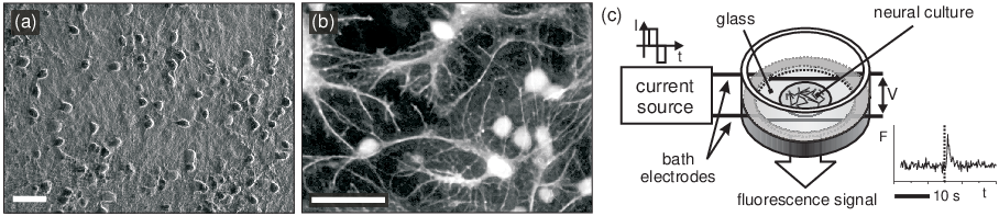
Experiments (see Ref. [10] for details) were performed on primary cultures of rat hippocampal neurons, that are plated on glass coverslips (Fig. 1a). Neurons develop dendrites and axons shortly after plating, creating a dense web of connections in a few days (Fig. 1b). Cultures were used 14–20 days after plating, when the network is fully developed and its activity is governed by the balance between excitatory and inhibitory neurons. About of the neurons are known to be inhibitory [11].
Neurons were electrically stimulated through bath electrodes (Fig. 1c), and the corresponding voltage drop measured with an oscilloscope. Neuronal activity was monitored using fluorescence calcium imaging, and data processed to record the fluorescence intensity as a function of time. Neural spiking activity is detected as a sharp increase of the fluorescence intensity.
The connectivity of the network was gradually weakened by blocking the AMPA glutamate receptors of excitatory neurons with the receptor antagonist CNQX. We studied the role of inhibition by either leaving active or blocking the GABA receptors with the corresponding antagonist bicuculine. For simplicity, we label the network containing both excitatory and inhibitory neurons by , and the network with excitatory neurons only by . The response of the network for a given CNQX concentration was quantified as the fraction of neurons that fired in response to the electric stimulation at voltage . Response curves were obtained by increasing the stimulation voltage from to V in steps of V. At the end of the experiments, the culture was washed of CNQX to verify that the initial network connectivity was recovered.
3 Model
We consider a simplified model of the network in terms of bond–percolation on a graph. The neural network is represented by the directed graph . Our main simplifying assumption is the following: A neuron has a probability to fire as a direct response to the electric excitation, and it always fires if any one of its input neurons fire (Fig. 2a). This approach ignores the fact that more than one input is needed to excite a neuron, and that connections are gradually weakened rather than abruptly removed. However, the aim of the model is to provide the simplest scenario to understand the experimental observations, and not the actual, highly complex behavior of neural cultures. is the natural unit in which to measure the response of the network, and by a change of variable the measured response curves can be expressed as .
The fraction of neurons in the network that fire for a given value of defines the firing probability . increases with the connectivity of , because any neuron along a directed path of inputs may fire and excite all the neurons downstream (Fig. 2a). All the upstream neurons that can thus excite a certain neuron define its input–cluster or excitation–basin. It is therefore convenient to express the firing probability as the sum over the probabilities of a neuron to have an input–cluster of size (Figs. 2b–c),
| (1) | |||||
where we used the probability conservation . increases monotonically with and ranges between and . The deviation of from linearity manifests the connectivity of the network (for disconnected neurons ). Eq. (1) indicates that the observed firing probability is actually one minus the generating function (or the –transform) of the cluster–size probability [12],
| (2) |
where . One can extract from the input–cluster size probabilities , formally by the inverse –transform, or more practically, in the experiments, by fitting to a polynomial in .

Once a giant component emerges (Fig. 2d) the observed firing pattern is significantly altered. In an infinite network, the giant component always fires no matter what the firing probability is. This is because even a very small is sufficient to excite one of the infinitely many neurons that belong to the giant component. We account for this effect by splitting the neuron population into a fraction that belongs to the giant component and always fires and the remaining fraction that belongs to finite clusters. This modifies the summation on cluster sizes into
| (3) |
As expected, at the limit of almost no self–excitation only the giant component fires, , and monotonically increases to . With a giant component present the relation between and the firing probability changes, obtaining
| (4) |
The size of the giant component decreases with the connectivity. At a critical connectivity the giant component disintegrates and its size is comparable to the average cluster size in the neural network. This behavior corresponds to a percolation transition, separating a system of small, fragmented clusters to one with a fast growing giant cluster that comprises most of the network.
4 Experimental results
Examples of the response curves for and networks are shown in Figs. 3a and 3b. At one extreme, with [CNQX] the network is fully connected. All neurons form a single cluster that comprises the entire network. A few neurons with low firing threshold suffice to activate the entire culture, leading to a very sharp response curve. At the other extreme, with high concentrations of CNQX ( 10 M) the network is completely disconnected, and the response curve is given by the individual neurons’ response. for individual neurons (denoted as ) is well described by an error function . This indicates that the firing threshold of a neuron in the network follows a gaussian distribution with mean and width .
Intermediate CNQX concentrations induce partial blocking of the synapses. Some neurons break off into separated clusters, while a giant cluster still contains most of the remaining neurons. The response curves are then characterized by a big jump that corresponds to the biggest cluster (giant component), and two tails that correspond to smaller clusters of neurons with low or high firing threshold. Beyond a critical concentration (around nM for networks and nM for networks) a giant component cannot be identified and the whole response curve is then also well described by an error function.

The biggest cluster in the network characterizes the giant component . For each response curve, is measured as the biggest fraction of neurons that fire together in response to the electric excitation, as shown by the grey bars in Figs. 3a and 3b. The size of the giant component was studied as a function of the connectivity probability (or synaptic strength) between two neurons [10], given by , with nM, and takes values between (full blocking) and (full connectivity).
The breakdown of the network for both and networks is shown in Fig. 3c. The giant component for networks breaks down at much lower CNQX concentrations compared with networks, indicating that the effect of inhibition on the network is to effectively reduce the number of inputs that a neuron receives on average. The behavior of the giant component indicates that the neural network undergoes a percolation transition, described by the power law . Power law fits for and networks give the same within the experimental error (Fig. 3d), indicating that is an intrinsic property of the network.
Finally, we have studied the size distribution for clusters that do not belong to the giant component. has been obtained by constructing the experimental function and after fitting a polynomial . Since is the response curve for individual neurons (Figs. 3a and 3b) and , the function for each response curve is obtained by plotting as a function of . For curves with a giant component present, its contribution is eliminated and the resulting curve normalized by the factor . Fig. 3e shows the functions for the response curves of Fig. 3a. The corresponding distribution, obtained from fits up to order , is shown in Fig. 3f. Overall, the clusters start out relatively big to rapidly become smaller for gradually higher concentrations of CNQX. is characterized by isolated peaks, indicating that loops and strong locality may be present in the neural culture. An example that illustrates the strong effect of loops on is shown in Fig. 2c. Since is obtained by fitting polynomials on , the accuracy in the description of is limited by the resolution of which, in turn, is limited by the experimental resolution in . In addition, since is a probability distribution, the fit is carried out with two constraints, reducing the freedom of fitting: the coefficients have to be positive and their sum has to be one. Hence, the distribution presented in Fig. 3f shows the correct behavior, but not the precise details of the distribution of input–clusters.
5 Numerical simulations
The model has been derived from classic bond percolation theory and has an analytic solution that yields precise results. However, the model contains a series of simplifying assumptions that may have an effect on the results. The numerical simulations that we present next are oriented to investigate the effect of removing or relaxing these assumptions, and to provide a physical picture for the connectivity in the network.
Three assumptions of the model are unrealistic. First, it assumes that one input suffices to activate a neuron, while in reality a number of input neurons must spike for the target neuron to fire. Second, the effect of CNQX is to bind and block AMPA glutamate receptor molecules, and consequently to continuously reduce the synaptic strength, so that bonds are in reality gradually weakened rather than abruptly removed. Third, the model assumes a tree-like connectivity, while in the living culture loops and clusters may exits. The numerical simulations have been applied to test that none of these assumptions change the main results of the model, i.e. that the giant component undergoes a percolation transition at a critical connectivity , and that the analysis of provides the distribution of input–clusters in the network.
The numerical simulations also provide the framework to study different degree distributions and their effect in the critical exponent . A Gaussian distribution gives , as in the experiments, while a power law distribution, , gives equal to or larger than one, where its exact value depends on the exponent [13].
5.1 Numerical method
The neural network was simulated as a directed random graph in which each vertex is a neuron and each edge is a synaptic connection between two neurons [14]. The graph was generated by assigning to each edge an input/output connectivity according to a predetermined degree distribution. Next, a connectivity matrix was generated by randomly connecting pairs of neurons with a link of initial weight 1 until each vertex was connected to links. The process of gradual weakening of the network was simulated in one case by removing edges, and in the second case by gradually reducing the bond strength from to . The connectivity is defined for the case of removing bonds as the fraction of remaining edges, and for the case of weakening bonds as the bond strength.
Each neuron has a threshold to fire in response to the external voltage, and all neurons have a threshold to fire in response to the integrated input from their neighbors. Since the experiments show that the probability distribution for independent neurons to fire in response to an external voltage is Gaussian, the ’s are distributed accordingly. For the simple case of removing links, the global threshold differentiates networks where a single input suffices to excite a target neuron from those where multiple inputs are necessary. When links are weakened plays a more subtle role, and determines the variable number of input neurons that are necessary to make a target neuron spike.
The state of each neuron, inactive () or active () was kept in a state vector . In the first simulation step, a neuron fires in response to the external voltage if the “excitation voltage” is greater than its individual threshold , i.e. .
In the subsequent simulation steps, a neuron fires due to the internal voltage if the integration over all its inputs at a given iteration is larger than : . The simulation iterates until no new neurons fire. The network response is then measured as the fraction of neurons that fired during the stimulation. The process is repeated for increasing values of , until the entire network gets activated, . Then, the network is weakened and the exploration in voltages started again.

5.2 Simulations results
5.2.1 Analysis of the model
To study the validity of the model, we have first considered 4 different situations: removing or weakening edges, and for or . In all cases the connectivity is set to be Gaussian for both input and output degree distributions. The results of the simulation are presented in Fig. 4. All 4 studied cases give qualitatively similar results, with response curves that are comparable to the ones observed experimentally, and with a giant component clearly identifiable. The analysis of the percolation transition gives in all 4 cases, in agreement with the value measured experimentally. As expected, the simulations with weakening bonds and for (five spiking neurons required to excite the target neuron) provide the response curves that are more similar to the ones observed experimentally. However, it is remarkable that the simplest case of the model (breaking bonds with ) already gives valid results. This indicates that, with the limitations of the model, the percolation approach proves to be remarkably powerful in describing the behavior observed experimentally.
The other important assumption of the model is the effect of the presence of loops in the network. Although loops are very rare in a random (Erdös-Rényi) graph, the connectivity in neural cultures is not random, and locality and neighboring probably may play an important role. However, graph theory tells us that most loops will be found in the giant component, where all neurons anyway light up and their effect is therefore irrelevant to our analysis. Clusters outside the giant component are in general tree–like, and thus the important analysis to be considered is what happens when finite clusters do have loops. The simulations show that the response curves and the percolation transition are not significantly altered if loops are allowed, providing similar results to the ones shown in Fig. 4.
Loops, however, do affect the clusters size distribution , which is then characterized by the presence of isolated peaks. To explore to which extent was sensitive to loops, we performed simulations considering different levels of clustering. The first graph that we analyzed was one with an artificially induced highly clustered connectivity. We generated a network where most of the links are located in highly connected clusters, with only weak connections between clusters. The distribution obtained from the breakdown of the connectivity in such a clustered network showed that the position of the dominant peaks corresponded to the size of the highly connected clusters. Next, having demonstrated the importance of highly connected clusters, we went on to consider realizations of the graph that would be more similar to the experimental network. To do that, we introduced the notion of geometry and of distance, placing all vertices on a spatial grid. Three different configurations were used: (i) a Gaussian connectivity with no locality, (ii) a Gaussian connectivity with local connections and (iii) a Gaussian connectivity with distance dependent link strength. For the first case no dominant peaks where identifiable. For the second one the existence of isolated peaks is more apparent. But for the third case the reinforced connectivity significantly increases the probability to have isolated input–clusters, similar to what we observe experimentally.
5.2.2 Role of inhibition and analysis of H(x)
We have studied the role of inhibition in the network by randomly selecting a subgroup of nodes and assigning them negative weights to simulate inhibitory neurons. Then, simulations with the same conditions described above were repeated and different excitation/inhibition ratios explored. The results indicate that the critical exponent is independent of the balance between excitation and inhibition, in agreement with the experimental observations. The results also show that the critical connectivity at which the giant component disintegrates does depend on the number of inhibitory neurons, and that this is a linear dependence.
Finally, we have verified with the simulations that the cluster distribution obtained from the polynomial fit of does not differ significantly from the distribution directly extracted from the connectivity matrix . Small deviations are a consequence of the constraints and in the polynomial fits, and in the uncertainty in removing the contribution of the giant component in the functions. This analysis gives validity to the distribution measured experimentally.
6 Discussion and conclusions
By comparing the exponent measured experimentally with the one obtained from the simulations we conclude that the connectivity in the neural culture is Gaussian. Simulations, however, are based on a random graph, while the real neural network is not, and one may think that the neural culture is actually better described by a two–dimensional, lattice–like network. Percolation on two–dimensional lattices gives a critical exponent , independent on the lattice structure. The value of the exponent increases rapidly with the dimensionality of the lattice, with and for three and four dimensions, respectively. In a system described by a 2–D structure, additional dimensions can be viewed as a gradual increase of long–range correlations.
The physical picture that we think may exist in the neural culture is that neurons are essentially connected to their neighbors, but with some long–range correlations. Axons can easily extend m in a neural culture, connecting neurons as far as cell bodies. The concept that locality is important is in fact quite natural when one thinks of the nature of the culture. Neurons are distributed homogeneously over the glass, and most likely all neurons start to form connections at the same time and at the same rate. This hints at a structure where neurons are highly connected with their neighbors. This is also suggested by the distribution of input–clusters , which shows that neurons are highly connected between them even after the giant component has begun disintegrating, forming local clusters with a significant presence of loops. We have also seen that neurons surrounded by many others tend to fire first in response to the external excitation, and that aggregates of neurons tend to fire together, with their collective response maintained even when the connectivity is reduced.
In summary, we have presented experimental results on the connectivity in neural cultures, and showed that connectivity undergoes a percolation transition characterized by a critical exponent . The experimental results were studied in the framework of percolation on a graph, and extracted the distribution of connected components in the network. Numerical simulations of the model were used to construct a physical picture of the connectivity in the neural network, and showed that the connectivity is characterized by a Gaussian degree distribution, with strong locality and clusterization.
References
- (1) V. B. Mountcastle, Brain 120, 701 (1997).
- (2) T. Binzegger, R. J. Douglas, and K. A. C. Martin, J. Neurosci. 24, 8441 (2004).
- (3) O. Sporns, D. R. Chialvo, M. Kaiser, and C. C. Hilgetag, Trends Cogn. Sci. 8, 418 (2004).
- (4) V. M. Eguíluz, D. R. Chialvo, G. A. Cecchi, M. Baliki, and A. V. Apkarian, Phys. Rev. Lett. 94, 018102 (2005).
- (5) J. G. White, E. Southgate, J. N. Thomson, and S. Brenner, Phil. Trans. R. Soc. Lond. B 314, 340 (1986).
- (6) M. E. J. Newman, The structure and function of complex networks, SIAM Review 45, 167 (2003).
- (7) M. E. J. Newman, A. L. Barabási, D. J. Watts, The Structure and Dynamics of Networks. (Princeton University Press, 2006).
- (8) D. Stauffer and A. Aharony, Introduction to Percolation Theory, 2nd Ed. (Taylor & Francis, London, 1991).
- (9) D. S. Callaway, M. E. J. Newman, S. H. Strogatz, D. J. Watts, Phys. Rev. Lett. 85, 5468 (2000).
- (10) I. Breskin, J. Soriano, E. Moses, T. Tlusty, Phys. Rev. Lett., in press (October 2006).
- (11) S. Marom and G. Shahaf. Q. Rev. Biophys. 35,63 (2002).
- (12) F. Harary and G.E. Uhlenbeck. Proc. Nat. Acad. Sci. 39 315 (1952); V.K.S. Shante and S. Kirkpatrick. Adv. Phys. 20, 325 (1971).
- (13) N. Schwartz, R. Cohen, D. ben-Avraham, A.-L. Barabási, S. Havlin, Phys. Rev. E 66, 015104(R) (2002).
- (14) M. E. J. Newman, S. H. Strogatz, D. J. Watts, Phys. Rev. E 64, 026118 (2001).