Decentralized Dynamic Hop Selection and Power Control in Cognitive Multi-hop Relay Systems

Liangzhong Ruan, stevenr@ust.hk
Vincent K.N. Lau, eeknlau@ee.ust.hk Affiliation: Dept. of Electrical and Electronic Engineering
the Hong Kong University of Science and Technology
Clear Water Bay, Kowloon, Hong Kong

Abstract

In this paper, we consider a cognitive multi-hop relay secondary user (SU) system sharing the spectrum with some primary users (PU). The transmit power as well as the hop selection of the cognitive relays can be dynamically adapted according to the local (and causal) knowledge of the instantaneous channel state information (CSI) in the multi-hop SU system. We shall determine a low complexity, decentralized algorithm to maximize the average end-to-end throughput of the SU system with dynamic spatial reuse. The problem is challenging due to the decentralized requirement as well as the causality constraint on the knowledge of CSI. Furthermore, the problem belongs to the class of stochastic Network Utility Maximization (NUM) problems which is quite challenging [21]. We exploit the time-scale difference between the PU activity and the CSI fluctuations and decompose the problem into a master problem and subproblems. We derive an asymptotically optimal low complexity solution using divide-and-conquer and illustrate that significant performance gain can be obtained through dynamic hop selection and power control. The worst case complexity and memory requirement of the proposed algorithm is ${\cal O}(M^{2})$ and ${\cal O}(M^{3})$ respectively, where $M$ is the number of SUs.

I Introduction

Cooperative Communication and Dynamic Spectrum Access (DSA) are two important technologies that drive the evolution of the next generation wireless systems. For instance, cooperative communication [1, 2] exploits the broadcast nature of the wireless channel and enhances the reliability of the packet against channel fading and hence, increases the coverage of wireless systems. There are a lot of works studying multi-hop relay network. In [3], the authors analyzed the performance of a dual-hop relaying communications over fading channels. Performance bounds of multi-hop relay system is analyzed in [4]. However, these works did not consider dynamic resource adaptation in the relay system. In [5], the authors investigated the minimum energy per bit treating both capacity and power consumption as optimization parameters in the wireless ad-hoc network. The minimization of the transmit power under the assumption of orthogonal transmissions was studied in [6, 7], in which the optimal parallel-relay channel power allocation for Amplify and Forward (AF) and Decode and Forward (DF) were derived. However, in all these works, the power control solution adapts on the path loss only and failed to exploit the dynamic fluctuations of microscopic fading. In [8], the authors considered dynamic power control for multi-hop relay but the solution is centralized and requires knowledge of the global channel state information about the entire adhoc network, which is very difficult to realize in practice. Furthermore, a fixed number of hops to deliver a packet to the destination is always assumed in the above works. Due to the store-and-forward penalty in the end-to-end throughput of multi-hop relaying, it is not always optimal to involve a fixed number of hops in the multi-hop network. To tackle this issue, various opportunistic multi-hop relaying protocols were proposed in [9, 10, 11]. In these designs, the number of hops to deliver a packet to the destination node changes dynamically according to the channel conditions. However, in these works, the opportunistic multi-hop protocols are heuristic in nature and the performance is studied by simulation and empirical measurements. In [12], performance analysis on one-hop relay protocol is studied. In [13, 14], performance analysis on some simple opportunistic multi-hop relaying protocols is studied. Furthermore, they all assume constant transmit power and deterministic channels where the effects of random fading is ignored.

On the other hand, DSA is an important new paradigm of spectrum access in which a secondary system dynamically shares medium with a higher priority primary system. Using cognitive radios (CRs) [15, 16], the nodes in the secondary user (SU) systems sense the activity of the primary users (PUs) and access the spectrum only if the primary system is idle. In other words, the SU system dynamically share the spectrum with the PU systems by exploiting the burstiness of the PU traffic in the temporal, frequency and spatial domains. One key issue of DSA or CR is the efficiency of spectrum sharing between the SU and PU systems. In [17, 18], the authors considered a CR system based on the interference avoidance approach in which the SU could transmit only if there are no active PUs within the coverage of the SU system. While such approach exploits the burstiness of the PU activity without requiring the knowledge of PU signal structure, the access opportunity of the SU system will be quite low for SU separated by a large distance as such access opportunity exists only if all the PU along the SU coverage are idle simultaneously. As a result, cognitive multi-hop relay for the SU systems is a promising solution to resolve this issue of low probability of access for distant secondary users. While intuitively, cognitive multi-hop relay could significantly enhance the spectrum sharing efficiency between the SU and PU systems, there are still a number of technical challenges to overcome as listed below.

•

Jointly Optimal Opportunistic Hop Selection and Power Control for Cognitive Multi-hop relays: Most of the existing works only considered either the power control [6, 7] or the opportunistic multi-hop relaying protocols. It is very important to jointly optimize both the forward hopping strategy and the power control policy to exploit the instantaneous fluctuations of PU activities and the microscopic fading in order to improve the performance of the cognitive multi-hop relays.
•

Dynamic Spatial Reuse in Cognitive Multihop Relaying: In most of the existing works studying power control or forward hopping in multihop relay [9, 10, 11], they focus entirely on the multihop aspects of the problem and assume that the multi-hop network does not have to share spectrum with any PU systems. This simplifies the problem significantly. While this is a reasonable assumption in the regular multihop network without PU, such symmetric spatial reuse is not always possible in cognitive multihop relay network due to the random PU activities on any hops.
•

Decentralized Solution with Local Knowledge of Channel State Information (CSI): An additional level of difficulty in solving the forward hopping and power control problem is the requirement of decentralized solution. In practice, it is very difficult to obtain and keep track of an up-to-date knowledge of the instantaneous channel state information for the entire multi-hop network. As a result, it is desirable to have a decentralized solution which requires knowledge of local (rather than global) channel state information only. In [20], the authors considered a distributed resource management scheme for multi-hop CR networks but no power control is considered and the solution is based on heuristic design.
•

Causal Knowledge of Channel States in the Multi-hop Relay Network: In most of the existing works [8], not only global knowledge but also non-causal¹¹ 1 Causality here refers to whether the source knows about the future channel states along the entire multihop transmission event from the source to the destination. In existing works, one way to justify the ”non-causal knowledge” is to assume the channel state remains quasi-static across the sum of frame durations in the multihop transmission from the source to the destination. knowledge of channel states in the multi-hop network is assumed. Specifically, at $t=0$ , the centralized controller is assumed to have knowledge of all the channel states in all the hops of the entire multi-hop relay network. However, by the time the packets are delivered in the $n$ -th hop, the actual channel state may have changed and the constraint of having causal knowledge of channel states have not been taken into account in the previous works of power optimization in multihop relay network.

In this paper, we shall try to address the above technical challenges. We consider a cognitive multi-hop SU system with a source, a destination and $M$ half-duplex cognitive relays scattered between the source and the destination. The SU system dynamically shares the spectrum with a PU system (with many PU nodes). The transmit power of the SU nodes as well as the hopping sequence of the cognitive relays are adaptive according to the local (and causal) knowledge of channel states in the multi-hop SU system to optimize the average end-to-end throughput. The solution also accommodates dynamic spatial reuse across the cognitive multi-hop system. The problem belongs to the class of stochastic NUM²² 2 Stochastic NUM refers to a Network Utility Maximization problem where the objective function involves expectation w.r.t. the stochastic system state and the optimization variables involve not just actions at a given system state realization but rather a collection of actions for all system state realizations. This is a challenging problem because of the huge dimension of variables involved as well as the lack of explicit closed form expression for the objective function in terms of the control policy. problems, which is well-known to be challenging. To obtain a decentralized solution for the throughput optimization problem we exploit the time-scale difference between the PU activity and the CSI fluctuations and decompose the problem into a master problem and subproblems (operating at different time scales). To deal with the causality requirement³³ 3 In our paper, we allow the CSI to be time varying across different hops in the multi-hop transmission and the control policy is adaptive to the current information (but not the future CSI knowledge) only., we express the subproblems into recursive forms and solve them using divide-and-conquer. We show that significant performance gains on the throughput of the SU system can be obtained using joint forward hopping and power control over a wide range of PU activity. Furthermore, we show that the decentralized solution has worst case complexity of ${\cal O}(M^{2})$ and is asymptotically optimal for large $M$ .

II System Model, Control Policy and End-to-End Throughput

Fig.1 illustrates the system model of the cognitive multi-hop relay system. The SU system consists of a cognitive source, a destination and several randomly distributed relays.

Assumption II.1

The system adopts certain Layer 3 (network layer) protocol to determine a route from the SU source node to the SU destination node, where the route is defined as a sequence of ordered nodes $\mathbb{R}=<R_{0},R_{1},...R_{M}>$ , where $R_{0},R_{M}$ are source node and destination node respectively. This route is assumed to be fixed throughout the communication session.

Denote the source as $R_{0}$ , destination $R_{M}$ and $M-1$ cognitive relays, $\{R_{1},...,R_{M-1}\}$ , which are distributed between $R_{0}$ and $R_{M}$ . The PU system consists of short-range wireless systems where the PU nodes are assumed to distribute uniformly (with a density of $\rho_{p}$ ) over the SU coverage area. Each of the PU node is assumed to have bursty activity with an active probability of $P_{a}$ . The PU and the SU systems share common frequency spectrum and the SU system can access the channel only when all the involved PU nodes are idle. In the following, we shall elaborate on the channel model, control policy and the end-to-end throughput of the SU cognitive multi-hop relay system.

II-A Channel Model

Figure 2 illustrates the signaling flow in multi-hop relay system. For the sensing of PU activity, we adopt the distributed sensing and centralized data fusion model as in IEEE 802.22. For instance, there are periodic quiet periods in the SU system that enable the sensing of PU activity. During the quiet periods, the SUs sense the PU activity locally and sends the sensing results to the other SU nodes. The SUs exchange the sensing results and update continuous segment (to be defined in the next subsection) information for data fusion. Define $A_{m}\in\{0,1\}$ as the sensing result which represents the availability of the shared spectrum to the SU system ( $A_{m}=1$ denotes that the shared spectrum is available to SU node $R_{m}$ ) and $\mathbf{A}=(A_{1},...,A_{m})$ be the vector of PU activity states for the $M$ SU nodes. We assume an SU node $R_{m}$ , $m=\{0,1...,M\}$ has access ( $A_{m}=1$ ) to the shared spectrum if and only if the nearest active PU node is at least $D_{0}$ meters away from the SU node⁴⁴ 4 $D_{0}$ is determined by the mean interference constraint to PU. For instance, denote $P_{int}$ as the interference constraint from SU to PU, $P_{0}$ is the mean transmitting power of SU, then $D_{0}\geq\left(\frac{P_{0}}{P_{int}}\right)^{\frac{1}{\alpha}}$ , where $\alpha$ is the path loss factor.. Furthermore, assume that $\mathbf{A}$ remains quasi-static between two consecutive sensing periods. This is a reasonable assumption as the burstiness of the PU nodes are of a longer time scale compared to the packet frame duration.

The received signal at the $j$ -th SU node from the $i$ -th SU node at the $k$ -th frame is given by:

\displaystyle Y_{ij}(k)={\color[rgb]{0,0,0}H_{ij}(k)\sqrt{D_{ij}}}X_{ij}(k)+Z_{ij}

(1)

where $X_{ij}(k)$ is the transmitted data symbol from node $i$ to node $j$ , $Z_{ij}$ is the zero-mean complex Gaussian channel noise (with normalized variance 1) and $G_{ij}(k)=|H_{ij}(k)|^{2}D_{ij}$ is the combined channel loss (including both the large-scale path loss $D_{ij}$ and the microscopic fading $H_{ij}$ ) between node $i$ and $j$ . The microscopic fading $H_{ij}$ is modeled as zero-mean, unit-variance complex Gaussian i.i.d (independent for different users) random variables. Let $\mathbf{G}(k)=\{G_{ij}(k):i\neq j,i,j\in\{0,1,...,M\}\}$ be the global channel state (GCS) information. We assume $\mathbf{G}$ is quasi-static within a frame. For practical considerations, we have the following restrictions on the knowledge of the channel states.

•

Local Knowledge of Channel States: We assume each of the SU node only has knowledge of the local channel state (LCS, to be defined below) and global PU activity state $\mathbf{A}$ (which remains quasi-static between two consecutive sensing periods).
•

Causal Knowledge of Channel States: We assume that each SU node only has causal knowledge of the LCS and cannot predict into the future.

Specifically, we assume at the $k$ -th frame, SU node m only has knowledge about the current LCS: $\mathbf{G}_{m}(k)$ . Here, $\mathbf{G}_{m}(k)=\{G_{mi}(k),i\in\{m+1,...,j\}\}$ in which $j$ should satisfy: $S_{m+1}=\ldots=S_{j}=1,S_{j+1}=0$ is the local CSI at the $k$ -th frame.

II-B System State, Hopping and Power Control Policy, System State Transition Kernel.

In this section, we shall formally define the control policy in the cognitive multi-hop relaying system. The multi-hop relay network operates in a DF manner with half-duplex constraint. At each frame, the upstream SU node transmits a packet of $B$ bits to its down-stream nodes using a transmit power which could be dynamically adjusted based on the current LCS knowledge. The down-stream SU node(s) attempt to decode the $B$ -bits packet before it can forward to the next hop.

In this paper we consider dynamic spatial reuse in the cognitive multi-hop relay system as illustrated in Figure 4. For any given PU states $\mathbf{A}$ , the multi-hop relay chain will be partitioned into several segments, which is defined as:

Definition II.1 (Continuous Segment in route $\mathbb{R}$ )

A continuous segment $L_{ij}$ in the cognitive multi-hop relay chain is defined as a sequence of nodes $<R_{i},...,R_{j}>\subseteq\mathbb{R}$ such that:

\displaystyle S_{i-1}=0,S_{i}=\ldots=S_{j}=1,S_{j+1}=0,\;\;i,j\in\{1,2...,M\}

(2)

(Define $S_{-1}=S_{M+1}=0$ ). The nodes $R_{i}$ and $R_{j}$ are called the head-node and the end-node of the continuous segment respectively. Define the probability of $\{R_{i},...,R_{j}\}$ forms a continuous segment as $\Pr(i,j)=\Pr(S_{i-1}=0,S_{i}=\ldots=S_{j}=1,S_{j+1}=0)$ . ∎

Spatial reuse is allowed only for relays in different segments of the partition. Hence, relays in different segments can transmit different information simultaneously without interfering each other. Packets are stored at the end-node of each continuous segment and the end-node are not allowed to transmit except when the down-stream PU activity becomes idle. However, for relays in one continuous segment, they have to obey the TDMA constraint and cannot transmit different information simultaneously at any given time.

Within a continuous segment $L_{ij}$ induced by the PU activity $\mathbf{A}$ , we shall define the hopping and power control policy as follows:

Definition II.2 (System State of Segment $L_{ij}$ )

Suppose $R_{i}\sim R_{j}$ induced by a continuous segment $L_{ij}$ under a PU activity state $\mathbf{A}$ . System state of $L_{ij}$ at frame index⁵⁵ 5 The frame index $k$ is equal to the number of hops already experienced by the packet currently transmitting in a continuous segment and will be reset to 1 when this packet is successfully delivered to the end node. Hence, $k$ might be different from segment to segment. $k\in\{1,2...j-i\}$ is given by: $\eta_{ij}(k)=\{s_{ij}(k),\mathbf{G}_{s_{ij}(k)}\}$ , where $s_{ij}(k)\in\{i,i+1,...j\}$ denotes the index of the source node at frame $k$ , $s_{ij}(1)=i$ ; $\mathbf{G}_{s_{ij}(k)}$ is the LCS at node $s_{ij}(k)$ . ∎

Definition II.3 (Control Policy $\Omega_{ij}$ in Segment $L_{ij}$ )

A stationary policy $\Omega_{ij}$ is a mapping from the current system state $\eta_{ij}(k)$ to the corresponding hopping and power control actions. The policy $\Omega_{ij}=\{\mathcal{L}_{ij},\mathcal{P}_{ij}\}$ , where:

•

Forward hopping policy $\mathcal{L}_{ij}$ : $l_{ij}(k)=\mathcal{L}_{ij}(\eta_{ij}(k)),k\in\{1,2...j-i\}$ , where the hopping control action (destination node index at frame $k$ ) has to satisfy the constraint: $s_{ij}(k)\leq l_{ij}(k)\leq j$ , with the left inequality strictly holds when $s_{ij}(k)<j$ .
•

Dynamic power control policy $\mathcal{P}_{ij}$ : $P_{ij}(k)=\mathcal{P}_{ij}(\eta_{ij}(k)),k\in\{1,2...j-i\}$ , where the power control action (transmitting power at frame $k$ ) shall satisfy $P_{ij}(k)>0$ .

∎

Definition II.4 (System State Transition Kernel)

The source node of at the $k+1$ -th frame $s_{ij}(k+1)$ , is determined by the hopping control action in the previous frame $l_{ij}(k)$ . Furthermore, the distribution of the channel state $\mathbf{G}_{s_{ij}(k+1)}$ is independent of the previous system states $\eta_{ij}(k)$ due to the casual knowledge assumption. Hence, the state transition kernel of the system state $\{\eta_{ij}(k)\}$ is given by:

\displaystyle\Pr(\eta_{ij}(k+1)|\eta_{ij}(k),\Omega_{ij})=\mathbf{1}\left(s_{ij}(k+1)=l_{ij}(k)\right)\cdot\Pr(\mathbf{G}_{s_{ij}(k+1)})

(3)

∎

Remark 1

Strictly speaking, the forward hopping policy $\mathcal{L}$ does not contain all possible hopping sequences w.r.t. a given route $\mathbb{R}$ . For example, potential loops (e.g. $R_{i}\rightarrow R_{j}\rightarrow R_{i}$ ) are excluded. Note that it is an intractable problem to optimize w.r.t. general hopping policies (including loops) due to the enormous possible policies involved. Instead, we shall restrict to forward hopping policy only and from which, we could exploit the structure in the policy space to derive much simpler solutions. ∎

II-C End-to-End Throughput with Dynamic Spatial Reuse and Forward Hopping Control

In order for a SU node to forward a packet, in any continuous segment, the node itself must be able to decode the packet first (DF). Suppose a node is able to decode if and only if the total mutual information received is no less than B bits. Hence, we have:

\displaystyle T_{ij}(k)\cdot\log(1+G_{s_{ij}(k)l_{ij}(k)}(k)P_{ij}(k))\geq B,\;\;k\in\{1,2...j-i\},s_{ij}<j

(4)

where $i,j$ satisfy (2) and $T_{ij}(k)$ is the transmitting time of the $k$ -th frame in continuous segment $L_{ij}$ . We first formally define the per-hop reward and cost below.

Definition II.5 (Per Hop Reward and Per Hop Cost)

Define the reward at the $k$ -th frame as the time taken to transmit 1 bit at the $k$ -th frame:

\displaystyle T(\eta_{ij}(k),\Omega_{ij})=\left\{\begin{array}[]{l}\frac{1}{\log(1+G_{s_{ij}(k)l_{ij}(k)}(k)P_{ij}(k))}\mbox{ when: }s_{ij}(k)<j\\ 0\mbox{ otherwise.}\end{array}\right.

Define the cost at the $k$ -th frame as the power consumed to transmit 1 bit at the $k$ -th frame:

\displaystyle P(\eta_{ij}(k),\Omega_{ij})=\left\{\begin{array}[]{l}\frac{P_{ij}(k)}{\log(1+G_{s_{ij}(k)l_{ij}(k)}(k)P_{ij}(k))}\mbox{ when: }s_{ij}(k)<j\\ 0\mbox{ otherwise.}\end{array}\right.

∎

Note that $T_{ij}(k)=B\cdot T(\eta_{ij}(k),\Omega_{ij})$ and hence the average data rate in the continuous segment $L_{ij}$ can be expressed as:

\displaystyle U_{ij}=E^{\Omega_{ij}}\left(\frac{B}{\sum_{k\in\{1,2...j-i\},s_{ij}(k)<j}T_{ij\_k}}\right)=E^{\Omega_{ij}}\left(\frac{1}{\sum_{k=1}^{j-i}T(\eta_{ij}(k),\Omega_{ij})}\right)

(11)

where the expectation $E^{\Omega_{ij}}$ is taken w.r.t. the probability measure induced by the control policy $\Omega_{ij}$ and the transition kernel in (3). Similarly, average power consumption $\overline{P}_{ij}$ in $L_{ij}$ can be expressed as:

\overline{P}_{ij}=E^{\Omega_{ij}}\left(\frac{\sum_{k=1}^{j-1}P(\eta_{ij}(k),\Omega_{ij})}{\sum_{k=1}^{j-i}T(\eta_{ij}(k),\Omega_{ij})}\right)

(12)

The end-to-end average throughput of the cognitive multi-hop system can be written as the weighted sum of average data rate of all continuous segments with end-node $R_{M}$ :

\overline{U}(\Omega)=\sum_{i=0}^{M-1}\Pr(i,M)U_{iM}

(13)

The average sum-power constraint is given by:

\sum_{i=0}^{M-1}\sum_{j=i+1}^{M}\Pr(i,j)\overline{P}_{ij}\leq P_{0}

(14)

Moreover, the conventional flow-balance constraint⁶⁶ 6 The conventional flow balance constraint ensures that the output flow does not exceed the input flow at any SU node. is given by:

\displaystyle\sum_{i=0}^{m-1}\Pr(i,m)U_{im}

\displaystyle\geq

\displaystyle\sum_{j=m+1}^{M}\Pr(m,j)U_{mj}\;\forall m\in\{1,...,M-1\}

(15)

III Problem Formulation

Note that the conventional flow-balance constraint in (15) may not be convex⁷⁷ 7 A convex (concave) function subtracting another convex (concave) function is neither convex nor concave in general.. To solve this issue, we introduce a new balance criteria, namely the section flow-balance criteria. For instance, we consider the sum of average data rate passing through each section (rather than each node). Specifically, the sum-average data rate passing through the $m$ -th section ( $m\in\{1,2,...M\}$ as illustrated in Fig.5). Define: $\bar{U}_{m}=\sum_{i=0}^{m-1}\sum_{j=m}^{M}\Pr(i,j)U_{ij}$ . The section flow-balance criteria is given by:

\overline{U}_{m}\geq\overline{U}_{m+1},\;\forall m\in\{1,...,M-1\}

(16)

In the following lemma, we shall illustrate that the section flow-balance criteria is in fact equivalent to the conventional per-node flow-balance:

Lemma III.1

[Equivalence of the flow balance criteria] The conventional per-node flow balance constraint in (15) is equivalent to the per-section flow balance criteria in (16).

Proof:

please refer to Appendix A for the proof. ∎

Lemma III.1 gives an equivalent form for traditional flow-balance criteria. Moreover, note that the objective $\overline{U}((\Omega))$ in (13) is equal to:

	$\displaystyle\overline{U}(\Omega)$	$\displaystyle=$	$\displaystyle\sum_{i=0}^{M-1}\Pr(i,M)U_{iM}\;=\sum_{i=0}^{M-1}\sum_{j=M}^{M}\Pr(i,j)U_{ij}\;=\bar{U}_{M}$		(17)
		$\displaystyle=$	$\displaystyle\min(\{\bar{U}_{1},\bar{U}_{2},...,\bar{U}_{M}\})\mbox{ (Due to section flow balance criteria (\ref{eqn:flow-balance2}))}$		(17)

where $\Omega$ is the overall control policy: $\Omega=\{\Omega_{ij},\forall i,j$ that satisfies (2) under a PU actively state $\mathbf{A}\}$ .

From (17), the optimization problem can be formulated as:

Problem 1 (Original Problem)

	$\displaystyle\bar{U}=\max_{\Omega}\left[\min_{m\in\{1,...,M\}}\sum_{i=0}^{m-1}\sum_{j=m}^{M}\Pr(i,j){U}_{ij}\right]$		(18)
	Subject to:
	$\displaystyle\sum_{i=0}^{M-1}\sum_{j=i+1}^{M}\Pr(i,j)\overline{P}_{ij}\leq P_{0}$		(19)

where: ${U}_{ij}$ , $\overline{P}_{ij}$ is given by (11) and (12) respectively.

III-A Decomposition of Main Problem

The optimization problem in (18) is too complex to solve directly. Furthermore, due to the causality constraint in the control policies ${\cal P}$ and ${\cal L}$ , the solution is not trivial and brute-force solution will not lead to viable solutions. However, it is worthy noting that for a given PU activity state $\mathbf{A}$ , operations on different continuous segment are naturally separated from each other. (e.g. as in Fig 4, when $S_{4}=0$ , hopping and power control policy in segment $R_{0}\sim R_{3}$ has no direct influence on that in $R_{5}\sim R_{6}$ ). Making use of this insight, we shall first decompose the problem into a master problem and a sub-problem. Define: ${\cal{P}}_{main}=\{\overline{P}_{ij}\},\;i,j\in\{0,1,...,M\},\;i<j$ .

We have the following decomposition theory:

Lemma III.2

Optimization problem consisting of a master problem ( Problem 2, with ${\cal{P}}_{main}$ as the optimization policy) and $\frac{M(M-1)}{2}$ subproblems (Problem 3, with ${\cal L}_{ij},{\cal P}_{ij}$ as the optimization policies) is equivalent to Problem 1.

Problem 2 (Master Problem)

	$\displaystyle\overline{U}=\max_{{\cal P}_{main}}\left[\min_{m\in\{1,...,M\}}\sum_{i=0}^{m-1}\sum_{j=m}^{M}\Pr(i,j){U}^{*}_{ij}(\overline{P}_{ij})\right]$		(20)
	Subject to:
	$\displaystyle\sum_{i=0}^{M-1}\sum_{j=i+1}^{M}\Pr(i,j)\overline{P}_{ij}\leq P_{0}$		(21)

Problem 3 (Subproblem)

	$\displaystyle{U}^{*}_{ij}(\overline{P}_{ij})=\max_{\mathcal{L}_{ij},\mathcal{P}_{ij}}E^{\Omega_{ij}}\left(\frac{1}{\sum_{k=1}^{j-i}T(\eta_{ij}(k),\Omega_{ij})}\right)$		(22)
	Subject to:
	$\displaystyle E^{\Omega_{ij}}\left(\frac{\sum_{k=1}^{j-1}P(\eta_{ij}(k),\Omega_{ij})}{\sum_{k=1}^{j-i}T(\eta_{ij}(k),\Omega_{ij})}\right)\leq\overline{P}_{ij}$		(23)

Proof:

Please refer to Appendix B for the proof. ∎

IV Decentralized Hop Selection and Power Control Algorithm

IV-A Solving the Sub Problem

To satisfy the causality constraint of the control policy on the local CSI, we have to model the subproblem in a recursive form so as to apply dynamic programming (DP) [22]. However, problem (22) cannot be expressed in a recursive form and hence, could not be divide-and-conquered. To tackle the challenges, we shall solve a lower bound version of the problem. We shall show that the lower bound solution is indeed asymptotically tight for large number of nodes.

IV-A1 Asymptotically Optimal Solution

We first elaborate a suboptimal solution for the subproblem (Problem 3). Let

\displaystyle\Omega_{ij}^{LB}=\arg\min_{\Omega_{ij}}E^{\Omega_{ij}}\left[\sum_{k=1}^{j-1}T(\eta_{ij}(k),\Omega_{ij})+\lambda_{ij}\left(P(\eta_{ij}(k),\Omega_{ij})-\overline{P}_{ij}T(\eta_{ij}(k),\Omega_{ij})\right)\right]

(24)

where the parameter $\lambda_{ij}$ in the suboptimal solution $\Omega_{ij}^{LB}$ is given by the roots of the equation⁸⁸ 8 For any given $\lambda_{ij}$ , $\Omega^{LB}_{ij}$ is determined by (24). Substitute both policy to the (25), the LHS become a function of $\lambda_{ij}$ :

E^{\Omega_{ij}}\left(\frac{\sum_{k=1}^{K_{ij}}P(\eta_{ij}(k),\Omega_{ij})}{\sum_{k=1}^{K_{ij}}T(\eta_{ij}(k),\Omega_{ij})}\right)=\overline{P}_{ij}

(25)

Note that the solution $\Omega_{ij}^{LB}$ is a feasible but suboptimal solution of the subproblem (Problem 3). We have the following lemma about the property of the suboptimal solution $\Omega_{ij}^{LB}$ .

Lemma IV.1 (Asymptotic Optimality of $\Omega^{LB}_{ij}$ )

If the following conditions are satisfied: 1) For any $\epsilon>0$ , there exists a finite $C>0$ such that when $|s-t|\geq C$ , $G_{st}<\epsilon$ ; and 2) $G_{st}\geq G_{st^{\prime}}$ , $G_{st}\geq G_{s^{\prime}t}$ when $t^{\prime}\geq t>s\geq s^{\prime}$ ; then we have: $U_{ij}^{LB}(\overline{P}_{ij})\rightarrow U^{*}_{ij}(\overline{P}_{ij})$ , as $|j-i|\rightarrow\infty$ . where $U_{ij}^{LB}(\overline{P}_{ij})$ is the average throughput of the segment $R_{i}\sim R_{j}$ using the suboptimal control $\Omega_{ij}^{LB}$ . ∎

Proof:

Please refer to Appendix C for the proof. ∎

Remark 2 ( Physical Interpretations of Conditions (1) and (2) in Lemma IV.1)

The condition 1) in Lemma IV.1 means that the nodes are not ”over concentrated” on one spot. This is is a mild requirement, which only excludes the special topologies where there are infinite number of nodes over a finite coverage area. The condition 2) refers to the path loss dominated situations, which applies for medium-range (over 2-5 km) multi-hop networks. ∎

As a result, the suboptimal solution $\Omega^{LB}_{ij}$ has reasonable performance in general cases (as will be illustrated in Section V) and it is asymptotically optimal for large number of nodes. In order to derive $\Omega^{LB}_{ij}$ , we shall first express into a recursive form and solve the problem by divide-and-conquer using DP. Define

g(\eta_{ij}(k);P_{ij}(k),l_{ij}(k))=\frac{1+\lambda_{ij}(P_{ij}(k)-\overline{P}_{ij})}{\log(1+P_{ij}(k)G_{s_{ij}(k)l_{ij}(k)}(k))}

(26)

then the problem (24) can be expressed recursively as:

J(s_{ij}(k))=E_{\mathbf{G}_{s_{ij}(k)}}[\min_{P_{ij}(k),l_{ij}(k)}(g(\eta_{ij}(k);P_{ij}(k),l_{ij}(k))+J(l_{ij}(k)))]

(27)

where $J(m)$ is called the expected cost from node $R_{m}$ to $R_{j}$ . Note that $J(j)=0$ and $J(s_{ij}(1))=J(i)$ gives the value of (24). As a result of the recursive form in (27), the backward recursion algorithm to solve problem (24) is summarized in the following.

Algorithm 1 (Offline and Online Solution of the Sub Problem)

• Offline Recursion: – Step 1: Initialize

\lambda_{ij}=0

. – Step 2: For

s=j-1,j-2,...,i

, determine

J(s)

by (Here we assume node

R_{s}

has the knowledge of the distribution of the local channel state

\mathbf{G}_{s}

J(s)=E_{\mathbf{G}_{s}(k)}\min_{m\in\{s+1,...j\}}\left[\frac{1+\lambda_{ij}(P_{s}^{*}(\lambda_{ij})-\overline{P}_{ij})}{\log(1+P_{s}^{*}(\lambda_{ij})G_{s,m}(k))}+J(m)\right]

(28) where

P^{*}_{s}(\lambda_{ij})

is the solution to (29) defined below. The values of

J(s)

is stored. – Step 3: Substitute solution obtained from Step 2 into (25). If the LHS is larger (smaller) than

\overline{P}_{ij}

\epsilon

, increase (decrease)

\lambda_{ij}

by a step

\delta

and go to Step 2. Otherwise, stop. • Online Policy: – Step 1: Set

k=1

and

s_{k}=i

. – Step 2: Obtain the local CSI

\mathbf{G}_{s_{ij}(k)}

and the optimizing hop selection and power control actions are given by

P^{*}_{s_{ij}(k)}(\lambda_{ij})

and:

l_{k}^{*}=\arg\min_{s\in\{l_{k}+1,...,j\}}\left[\frac{1+\lambda_{ij}(P_{l_{k}}^{*}(\lambda_{ij})-\overline{P}_{ij})}{\log(1+P_{ij}(k)^{*}(\lambda_{ij})G_{l_{k},s}(k))}+J(s)\right]

– Step 3: Set

k:=k+1

s_{k+1}=l_{k}^{*}

. If

s_{k+1}\neq j

, goto Step 2. Otherwise, stop.

\frac{G_{s_{ij}(k)l_{ij}(k)}(k)}{(1+P_{ij}(k)G_{s_{ij}(k)l_{ij}(k)}(k))\log(1+P_{ij}(k)G_{s_{ij}(k)l_{ij}(k)}(k))+(\overline{P}_{ij}-P_{ij}(k))G_{s_{ij}(k)l_{ij}(k)}(k)}=\lambda_{ij}

(29)

Remark 3

Note that the memory size of the table in the offline recursion is $j-i$ . The computational complexity for the online algorithm in each step $k$ is only of the order $j-i$ . Hence, the online algorithm has worst case complexity ${\cal O}(M^{2})$ and worst case memory requirement ${\cal O}(M)$ for each continuous segment $i,j$ . ∎

IV-B Solving the Main Problem

After solving for the subproblem, we shall focus on solving the main problem based on $U^{LB}_{ij}(\overline{P}_{ij})$ (which is of a longer time scale) in this section. We first establish the following Theorem regarding the concavity of $U^{LB}_{ij}(\overline{P}_{ij})$ w.r.t. $\overline{P}_{ij}$ .

Lemma IV.2 (Concavity of the Lower Bounds of $U^{*}_{ij}(\overline{P}_{ij})$ )

The lower bound ( $U^{LB}_{ij}(\overline{P}_{ij})$ ) of $U^{*}_{ij}(\overline{P}_{ij})$ is a concave function of $\overline{P}_{ij}$ .

Proof:

Please refer to Appendix E for the proof. ∎

From Lemma IV.2, it is easy to deduce that the lower-bound version of the master problem in (20) [with $U_{ij}^{*}(\overline{P}_{ij}$ ) replaced by $U_{ij}^{LB}(\overline{P}_{ij})$ ] is a convex optimization problem. As a result, the standard gradient search could be applied to solve the master problem. Please refer to Figure 10 for the detailed algorithm description.

Remark 4

Note that the offline recursion needs to be updated only when there are changes in the PU statistics or the SU path loss and in practice, the above offline algorithm is computed over a long time scale. Combining the master problem and the subproblems the total memory requirement of the offline table in algorithm 1 is $\mathcal{O}(M^{3})$ . ∎

V Simulation Results

In this section, we shall illustrate the performance of the proposed scheme by simulation. We consider a multi-hop cognitive relay system with $6$ nodes ( $\{R_{0},R_{1},...R_{5}\}$ ) and 6 PUs (one PU in the neighborhood of each SU node). The distance between $R_{0}$ and $R_{5}$ is 5, and the other 4 nodes randomly scatter between them. Path loss between two nodes $R_{i},R_{j}$ is given by the ”flat-earth model” [24]: $\log_{10}D_{ij}=-\alpha\log_{10}d_{ij}\;(dB)$ where $d_{ij}$ is the distance between the two nodes and $\alpha$ is the path loss exponent. The proposed scheme is compared with four schemes below:

•

Direct transmission only (Baseline 1): $R_{0}$ transmit directly to $R_{5}$ when all PU remain silent ( $S_{i}=1,\forall i\{0,1,...5\}$ ). This is equivalent to the case without relay.
•

Per-node transmission only (Baseline 2): if $R_{m}$ ( $\forall m\{0,1,...4\}$ ) received a packet in previous frames, it transmits this packet to $R_{m+1}$ when the PU activity permits ( $A_{m}=S_{m+1}=1$ ). This corresponds to the traditional DF multi-hop relay scheme.
•

Direct (per-node) transmission with dynamic spatial reuse (Baseline 3/4): These two schemes adopt the same dynamic spatial reuse method as the proposed scheme. Yet, within each continuous segment, they adopt direct and per-node transmission respectively.

Figure 6 and Figure 7 illustrate the average end-to-end throughput ( $\overline{U}$ ) versus the average SNR ( $P_{0}$ ) and PU activity level ( $\Pr(A_{m}=0)$ ) respectively. The proposed scheme achieves significant throughput gains over a wide range of SNR and PU activities. This gain is contributed by both the dynamic hop selection as well as dynamic power control. Comparison with baseline 1 illustrates how cognitive relay could help to increase the probability of access and efficiency of spectrum sharing in general. Comparison with baseline 2 and 3 illustrates the importance of joint dynamic power and opportunistic hop selection in cognitive multihop systems. The gain contributed by the dynamic hop selection is most significant under moderate SNR. At very high SNR, the dynamic hopping performance approaches that of the baseline 3, illustrating the system always perform one-hop direct transmission to avoid the half-duplex penalty. At very low SNR, the performance of the proposed scheme approaches that of the baseline 4, illustrating that the system prefer hop-by-hop transmission for SNR gain.

Figure 7 illustrate that the dynamic hopping gain is more prominent under low PU activity. This is because at low PU activity, there is a higher chance of forming a longer continuous segment and hence, more flexible choices for the dynamic hop selection. Figure 8 illustrate the convergence rate of the off-line recursion for the Main problem (Algorithm 2). The proposed algorithm can achieve $90\%$ of the converged performance within 10 iterations and converges after about 30 iterations. This iteration efficiency is good enough for off-line algorithms.

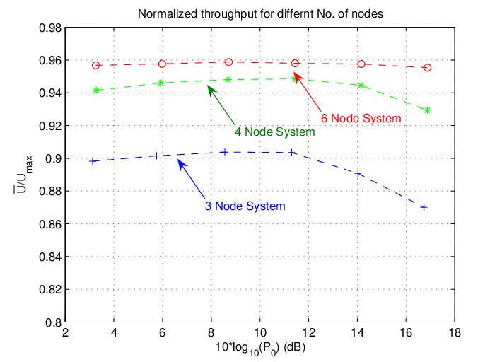
Figure 9 illustrates the normalized throughput $\frac{\bar{U}}{U_{max}}$ versus the average transmit SNR ( $P_{0}$ ) for various number of cognitive relay nodes where $\frac{\bar{U}}{U_{max}}$ is obtained from brute-force numerical optimization of Problem 1. With $N=6$ , we have over $95\%$ of the optimal performance. This illustrates that the proposed scheme is not only order-optimal but achieves close-to-optimal performance even in small to moderate number of cognitive relay nodes.

VI Summary

In this paper, we have derived a low complexity hop selection and dynamic power control policies to maximize the average end-to-end throughput of the cognitive multi-hop SU system with dynamic spatial reuse. By exploiting the time-scale difference between the PU activity and the CSI dynamics, we decompose the problem into a Master problem and several Sub Problems. The solution obtained is decentralized in the sense that each node determines its next hop and transmit power based on the local and causal CSI only. The solution consists of an offline recursion and an online algorithm with worst case complexity ${\cal O}(M^{2})$ and worst case memory requirement ${\cal O}(M^{3})$ . Furthermore, the solution is asymptotically optimal for large number of nodes. Significant throughput performance has been demonstrated.

Appendix A Proof of Lemma III.1

	$\displaystyle\bar{U}_{m}-\bar{U}_{m+1}$	$\displaystyle=$	$\displaystyle\sum_{i=0}^{m-1}\sum_{j=m}^{M}\Pr(i,j)U_{ij}-\sum_{i=0}^{m}\sum_{j=m+1}^{M}\Pr(i,j)U_{ij}$
		$\displaystyle=$	$\displaystyle\sum_{i=0}^{m-1}\Pr(i,m)U_{i,m}-\sum_{j=m+1}^{M}\Pr(m,j)U_{m,j}\;\;\;\;\;\forall m\in\{1,...,M-1\}$

Hence:

	$\displaystyle U_{m}\geq U_{m+1}$	$\displaystyle\Leftrightarrow$	$\displaystyle\sum_{i=0}^{m-1}\Pr(i,m)U_{i,m}-\sum_{j=m+1}^{M}\Pr(m,j)U_{m,j}\geq 0$		(30)
		$\displaystyle\Leftrightarrow$	$\displaystyle\sum_{i=0}^{m-1}\Pr(i,m)U_{i,m}\geq\sum_{j=m+1}^{M}\Pr(m,j)U_{m,j}$		(30)

Appendix B Proof of Lemma 3

To prove Problem 2 and Problem 3 are equivalent to Problem 1, we first prove the following Lemma:

Lemma B.1

Define:

	$\displaystyle V$	$\displaystyle=$	$\displaystyle\max_{\mathbf{X}}\min_{m\in\{1,2...M\}}\left(\sum_{i=1}^{L}A_{mi}f_{i}(x_{i})\right)$		(31)
	$\displaystyle V^{\prime}$	$\displaystyle=$	$\displaystyle\min_{m\in\{1,2...M\}}\max_{\mathbf{X}}\left(\sum_{i=1}^{L}A_{mi}f_{i}(x_{i})\right)$		(32)

where $\mathbf{X}=\{x_{i}\in\mathbb{C}_{i},i\in\{1,2...L\}\}$ are a set of independent variables. If $f_{i}(x_{i})$ is finite and $\forall m\in\{1,2...M\},i\in\{1,2...L\}$ , then:

\displaystyle V=V^{\prime}=\min_{m\in\{1,2...M\}}\left(\sum_{i=1}^{L}A_{mi}f^{*}_{i}\right)

(33)

where $f^{*}_{i}=\max_{x_{i}\in\mathbb{C}_{i}}f_{i}(x_{i})$ .

Proof:

In general, switching of ” $\max$ ” and ” $\min$ ” is not allowed but there are two specific structures in Lemma B.1. that we are exploiting.

•

Independency Property: $f_{i}(x_{i}),\forall i$ are mutually independent (i.e. they are not coupled by any common variables), as $\mathbf{X}=\{x_{i},i\in\{1,2...L\}\}$ is a set of independent variables.
•

Monotone Property: Since for every $m$ and $i$ , $A_{mi}\geq 0$ : $\forall m,i$ , $\sum_{i=1}^{L}A_{mi}f_{i}(x_{i})$ is an non-decreasing function of $f_{i}(x_{i})$ . As a result, $V$ is an non-decreasing function of $f_{i}(x_{i})$ , $\forall i\in\{1,2...L\}$ .

Since $V$ is an non-decreasing function of $f_{i}(x_{i})$ (Monotone Property), $f_{i}(x_{i})\leq f^{*}_{i}$ , $\forall i\in\{1,2...M\}$ :

\displaystyle V\leq\min_{m\in\{1,2...M\}}\left(\sum_{i=1}^{L}A_{mi}f^{*}_{i}\right)

(34)

Moreover, denote $x^{*}_{i}=\arg\max_{x_{i}\in\mathbb{C}_{i}}f_{i}(x_{i})$ , from the Independency Property, $\{x_{i}=x^{*}_{i},i\in\{1,2...M\}\}$ is a feasible point for $V$ . Hence:

\displaystyle V\geq\min_{m\in\{1,2...M\}}\left(\sum_{i=1}^{L}A_{mi}f^{*}_{i}\right)

(35)

Combining (34), (35) $V=\min_{m\in\{1,2...M\}}\left(\sum_{i=1}^{L}A_{mi}f^{*}_{i}\right)$ .

On the other hand, since $\forall m$ , $\max_{\mathbf{X}}\left(\sum_{i=1}^{L}A_{mi}f_{i}(x_{i})\right)=\sum_{i=1}^{L}A_{mi}f^{*}_{i}$ :

\displaystyle V^{\prime}=\min_{m\in\{1,2...M\}}\left(\sum_{i=1}^{L}A_{mi}f^{*}_{i}\right)

(36)

∎

In Problem 1, for a fixed $\mathcal{P}_{main}$ , denote:

$\displaystyle\overline{U}(\mathcal{P}_{main})$	$\displaystyle=$	$\displaystyle\max_{{\mathcal{L}},{\mathcal{P}}\|\mathcal{P}_{main}}\min_{m\in\{1,...,M\}}\left(\sum_{i=0}^{m-1}\sum_{j=m}^{M}\Pr(i,j){U}_{ij}\right)$	(37)
	$\displaystyle=$	$\displaystyle\max_{{\mathcal{L}},{\mathcal{P}}\|\mathcal{P}_{main}}\min_{m\in\{1,...,M\}}\left(\sum_{i=0}^{M-1}\sum_{j=1}^{M}A(i,j,m){U}_{ij}\right)$	(37)
where:		$\displaystyle A(i,j,m)=\left\{\begin{array}[]{l}\Pr(i,j)\;\;\mbox{if: }i<m\leq j;\\ 0\;\;\;\;\mbox{else}\end{array}\right.$

Note that: a) From (11), (12), $U_{ij}$ and $\overline{P}_{ij}$ depends on different set of variables ${\cal L}_{ij}$ and ${\cal P}_{ij}$ . Hence, for a given ${\cal{P}}_{main}=\{\overline{P}_{ij}\}$ , constraint (19) is decoupled and $\{\mathcal{L}_{ij},\mathcal{P}_{ij}\}$ become independent variables for different $\{i,j\}$ .

b) From (18), for all $i,j$ , $\Pr(i,j)\geq 0$ , $A(i,j,m)\geq 0$ , $\forall i,j,m$ .

Combining a) and b), we can apply Lemma B.1 and obtain:

\displaystyle\overline{U}({\mathcal{P}}_{main})

\displaystyle=

\displaystyle\min_{m\in\{1,...,M\}}\left(\sum_{i=0}^{m-1}\sum_{j=m}^{M}\Pr(i,j)U^{*}_{ij}(\overline{P}_{ij})\right)

(41)

where $U^{*}_{ij}(\overline{P}_{ij})$ is given by the solution of Problem 3. Hence, we can rewrite the objective function as:

\displaystyle\overline{U}=\max_{{\mathcal{P}}_{main}}\overline{U}({\mathcal{P}}_{main})=\max_{{\mathcal{P}}_{main}}\min_{m\in\{1,...,M\}}\left(\sum_{i=0}^{m-1}\sum_{j=m}^{M}\Pr(i,j)U^{*}_{ij}(\overline{P}_{ij})\right)

(42)

which is exactly the objective function in Problem 2. Therefore, the optimal solution given by Problem 2 and Problem 3 shall be the same as Problem 1.

Appendix C Proof of Lemma IV.1

We shall prove that the suboptimal solution $\Omega^{LB}_{ij}$ is asymptotically optimal under the two conditions in Lemma IV.1. We shall first prove the following Lemma:

Lemma C.1

Suppose: 1) For any

\epsilon>0

, there exists a finite

C>0

such that when

|s-t|\geq C

G_{st}<\epsilon

; 2)

G_{st}\geq G_{st^{\prime}}

G_{st}\geq G_{s^{\prime}t}

when

t^{\prime}\geq t>s\geq s^{\prime}

. Then:

\displaystyle\frac{\sum_{k=1}^{j-i}T(\eta_{ij}(k),\Omega_{ij})}{E^{\Omega_{ij}}\sum_{k=1}^{j-i}T(\eta_{ij}(k),\Omega_{ij})}\rightarrow 1\mbox{ and}

(43)

\displaystyle\frac{\sum_{k=1}^{j-i}P(\eta_{ij}(k),\Omega_{ij})}{E^{\Omega_{ij}}\sum_{k=1}^{j-i}P(\eta_{ij}(k),\Omega_{ij})}\rightarrow 1\mbox{ in probability when }|j-i|\rightarrow\infty

(44)

Proof:

We partition the continuous segment $R_{i}\sim R_{j}$ into $R=\lceil\frac{j-i}{C}\rceil$ clusters: $\mathbb{V}_{r}=\{i+rC,i+rC+1,...\min(i+r(C+1)-1,j)\}$ , $r\in\{0,1...R-1\}$ . As for any $\epsilon>0$ , there exists a finite $C>0$ such that when $|s-t|\geq C$ , $G_{st}<\epsilon$ , let $\epsilon\ll\frac{1}{\overline{P}_{ij}}$ , we have:⁹⁹ 9 Otherwise, $T(\eta_{ij}(k),\Omega_{ij})=\frac{1}{\log(1+G_{s_{ij}(k)l_{ij}(k)}(k)P_{ij}(k))}\sim\mathcal{O}\frac{1}{\epsilon\overline{P}_{ij}(k)}\rightarrow\infty$

\displaystyle l_{ij}(k)-s_{ij}(k)<C,\forall k\in\{1,2...j-i\}

(45)

Denote $T_{r}=\sum_{l_{ij}(k)\in\mathbb{V}_{r}}T(\eta_{ij}(k),\Omega_{ij})=\sum_{s_{ij}(k)\neq j,l_{ij}(k)\in\mathbb{V}_{r}}\frac{1}{\log(1+G_{s_{ij}(k)l_{ij}(k)}(k)P_{ij}(k))}$ , then: $\sum_{k=1}^{j-i}T(\eta_{ij}(k),\Omega_{ij})=\sum_{r=0}^{R-1}T_{r}$ . Moreover, from (45), we have: $1\leq|s_{ij}(k)\neq j,l_{ij}(k)\in\mathbb{V}_{r}|\leq C$ . Moreover, as in practice, the time duration to transmit one bit should be positive and finite, there should exist $T_{\min},T_{\max}\in\mathbb{R}^{+}$ such that $T_{\min}\leq T(\eta_{ij}(k),\Omega_{ij})\leq T_{\max}$ , $\forall\eta_{ij}(k)$ . Hence we have:

\displaystyle T_{\min}\leq T_{r}\leq CT_{\max},\forall r\in\{0,1,...R-1\}

(46)

As we shall proof in Appendix D, we have the following results concerning the covariance between $\{T_{r}\}$ :

Lemma C.2

Given: 1) For any

\epsilon>0

, there exists a finite

C>0

such that when

|s-t|\geq C

G_{st}<\epsilon

G_{st}\geq G_{st^{\prime}}

G_{st}\geq G_{s^{\prime}t}

when

t^{\prime}\geq t>s\geq s^{\prime}

. We have:

\mbox{Cov}(T_{r},\sum_{s=0}^{r-1}T_{s})\leq 0

\forall r\in\{1,2...R-1\}

. ∎

With Lemma C.2 and (46), we have:

	$\displaystyle\mbox{Var}(\frac{\sum_{r=0}^{R-1}T_{r}}{E^{\Omega_{ij}}\sum_{r=0}^{R-1}T_{r}})$	$\displaystyle=$	$\displaystyle\frac{\sum_{r=0}^{R-1}\mbox{Var}(T_{r})+2\sum_{r=1}^{R-1}\mbox{Cov}(T_{r},\sum_{s=0}^{r-1}T_{s})}{\left(\sum_{r=0}^{R-1}E^{\Omega_{ij}}T_{r}\right)^{2}}\leq\frac{\sum_{r=0}^{R-1}\mbox{Var}(T_{r})}{R^{2}T^{2}_{\min}}$		(47)
		$\displaystyle\leq$	$\displaystyle\frac{RC^{2}T^{2}_{\max}}{R^{2}T^{2}_{\min}}\rightarrow 0\;\;\mbox{as: }R=\lceil\frac{j-i}{C}\rceil\rightarrow\infty$		(47)

Substitute (47) into Chebyshev inequality, (43) is proved; (44) can also be proved through similar process. We shall omit the details due to page limit. ∎

From (43), (44):

	$\displaystyle E^{\Omega_{ij}}\left[\frac{1}{\sum_{k=1}^{j-i}T(\eta_{ij}(k),\Omega_{ij})}\right]\rightarrow\frac{1}{\sum_{k=1}^{j-i}E^{\Omega_{ij}}T(\eta_{ij}(k),\Omega_{ij})}\mbox{ and}$
	$\displaystyle E^{\Omega_{ij}}\left[\frac{\sum_{k=1}^{j-i}P(\eta_{ij}(k),\Omega_{ij})}{\sum_{k=1}^{j-i}T(\eta_{ij}(k),\Omega_{ij})}\right]\rightarrow\frac{\sum_{k=1}^{j-i}E^{\Omega_{ij}}P(\eta_{ij}(k),\Omega_{ij})}{\sum_{k=1}^{j-i}E^{\Omega_{ij}}T(\eta_{ij}(k),\Omega_{ij})}\mbox{ in probability when }j-i\rightarrow\infty$

Hence, for sufficiently large $j-i$ , Problem 3 can be equivalently rewritten as:

			$\displaystyle\min_{\Omega_{ij}}\sum_{k=1}^{j-i}E^{\Omega_{ij}}T(\eta_{ij}(k),\Omega_{ij})$		(48)
		S.t.:	$\displaystyle\sum_{k=1}^{j-i}E^{\Omega_{ij}}\left(P(\eta_{ij}(k),\Omega_{ij})-\overline{P}_{ij}T(\eta_{ij}(k),\Omega_{ij})\right)\leq 0$		(49)

Observe that the Lagrangian dual function of the above problem is exactly (24). Hence, $U^{LB}(\overline{P}_{ij})\rightarrow U^{*}_{ij}(\overline{P}_{ij})$ for sufficiently large $j-i$ .

Appendix D Proof of Lemma C.2

We shall first prove the following Lemma:

Lemma D.1

Given three sequences

a_{0}\leq a_{1}\leq...\leq a_{N}

b_{0}\geq b_{1}\geq...\geq b_{N}

p_{n}\geq 0,n\in\{0,1...N\}

which satisfy:

\sum_{n=0}^{N}p_{n}=1

\sum_{n=0}^{N}p_{n}a_{n}=\sum_{n=1}^{N}p_{n}b_{n}=0

, we have:

\sum_{n=0}^{N}p_{n}a_{n}b_{n}\leq 0

. ∎

Proof:

Denote $N^{-}_{a}=|\{n:a_{n}<0\}|$ , $N^{+}_{b}=|\{n:b_{n}>0\}|$ , where $|\mathbb{A}|$ means the cardinality or set $\mathbb{A}$ . If $N^{-}_{a}=N^{+}_{b}$ , then obviously $\sum_{n=0}^{N}a_{n}b_{n}\leq 0$ ; Otherwise, without loss of generality, assume $N^{-}_{a}>N^{+}_{b}$ and then:

	$\displaystyle\sum_{n=1}^{C}p_{n}a_{n}b_{n}=\sum_{n=0}^{N^{+}_{b}-1}p_{n}a_{n}b_{n}+\sum_{n=N^{+}_{b}}^{N^{-}_{a}-1}p_{n}a_{n}b_{n}+\sum_{n=N^{-}_{a}}^{N}p_{n}a_{n}b_{n}\leq\sum_{n=0}^{N^{+}_{b}-1}p_{n}a_{n}b_{n}+\sum_{n=N^{+}_{b}}^{N^{-}_{a}-1}p_{n}a_{n}b_{n}$
	$\displaystyle\leq a_{(N^{+}_{b}-1)}\sum_{n=0}^{N^{+}_{b}-1}p_{n}b_{n}+a_{(N^{+}_{b})}\sum_{n=N^{+}_{b}}^{N^{-}_{a}-1}p_{n}b_{n}\leq(a_{(N^{+}_{b}-1)}-a_{(N^{+}_{b})})\sum_{n=0}^{N^{+}_{b}-1}p_{n}b_{n}\leq 0$		(50)

∎

Recall the system state transition kernel:

\displaystyle\Pr(\eta_{ij}(k)|\eta_{ij}(k-1),\Omega_{ij})=\mathbf{1}\left(s_{ij}(k)=l_{ij}(k-1))\right)\Pr(\mathbf{G}_{s_{ij}(k)})

(51)

It can be observed that conditioned on the source node at the frame $k$ : $s_{ij}(k)$ , $\{\eta_{ij}(k),\eta_{ij}(k+1),...\}$ are independent of $\{\eta_{ij}(1),\eta_{ij}(2),...\eta_{ij}(k-1)\}$ . Correspondingly, $\{T(\eta_{ij}(s),\Omega^{ij}),s\in\{k,k+1...\}\}$ are conditionally independent of $\{T(\eta_{ij}(s),\Omega^{ij}),s\in\{1,2...,k-1\}\}$ . Denote $l_{r\_\min}=\min(l_{ij}(k):l_{ij}(k)\in\mathbb{V}_{r})$ . Then: conditional on $l_{r\_\min}$ , $T_{r}$ is independent of $\{T_{s},s\in\{0,1,...r-1\}\}$ . Hence:

\displaystyle E^{\Omega_{ij}}\left.\left(T_{r}\cdot\sum_{s=1}^{r-1}T_{s}\right|l_{r\_\min}=x\right)=E^{\Omega_{ij}}(T_{r}|l_{r\_\min}=x)E^{\Omega_{ij}}\left.\left(\sum_{s=1}^{r-1}T_{s}\right|l_{r\_\min}=x\right)

(52)

where $x\in\{i+rC,i+rC+1,...i+rC+|\mathbb{V}_{r}|-1\}$ . Denote $k_{r\_\min}=\min(k:l_{ij}(k)\in\mathbb{V}_{r})$ . Since $G_{st}\geq G_{st^{\prime}}$ when $s<t\leq t^{\prime}$ , $T(\eta_{ij}(k_{r\_\min})-1)$ is an non-decreasing function of $l_{r\_\min}$ . Correspondingly, $E^{\Omega_{ij}}\left.\left(\sum_{s=1}^{r-1}T_{s}\right|l_{r\_\min}\right)$ is a non-decreasing function of $l_{r\_\min}$ . Similarly, as $G_{st}\geq G_{s^{\prime}t}$ when $s^{\prime}\leq s<t$ , $E^{\Omega_{ij}}(T_{r}|l_{r\_\min})$ is a non-increasing function of $l_{r\_\min}$ . Let $E^{\Omega_{ij}}\left.\left(\sum_{s=1}^{r-1}T_{s}\right|l_{r\_\min}=x\right)-E^{\Omega_{ij}}\left(\sum_{s=1}^{r-1}T_{s}\right)=a_{x}$ , $E^{\Omega_{ij}}(T_{r}|l_{r\_\min}=x)-E^{\Omega_{ij}}(T_{r})=b_{n}$ , $\Pr(l_{r\_\min}=x)=p_{n}$ and substitute to Lemma D.1: $\sum_{x=i+rC}^{i+rc+|\mathbb{V}_{r}|-1}\Pr(l_{r\_\min}=x)\left(E^{\Omega_{ij}}(T_{r}|l_{r\_\min}=x)-E^{\Omega_{ij}}(T_{r})\right)\left(E^{\Omega_{ij}}\left.\left(\sum_{s=1}^{r-1}T_{s}\right|l_{r\_\min}=x\right)-E^{\Omega_{ij}}\left(\sum_{s=1}^{r-1}T_{s}\right)\right)\leq 0$ . From this result and (52):

	$\displaystyle\mbox{Cov}(T_{r},\sum_{s=0}^{r-1}T_{s})=E^{\Omega_{ij}}\left(T_{r}\sum_{s=1}^{r-1}T_{s}\right)-E^{\Omega_{ij}}\left(T_{r}\right)E^{\Omega_{ij}}\left(\sum_{s=1}^{r-1}T_{s}\right)$
	$\displaystyle=\sum_{x=i+rC}^{i+rc+\|\mathbb{V}_{r}\|-1}\Pr(l_{r\_\min}=x)\left(E^{\Omega_{ij}}(T_{r}\|l_{r\_\min}=x)-E^{\Omega_{ij}}(T_{r})\right)$
	$\displaystyle\;\;\;\;\cdot\left(E^{\Omega_{ij}}\left.\left(\sum_{s=1}^{r-1}T_{s}\right\|l_{r\_\min}=x\right)-E^{\Omega_{ij}}\left(\sum_{s=1}^{r-1}T_{s}\right)\right)\leq 0$		(53)

Appendix E Proof of Lemma IV.2

Due to the Theorem of Lagrangian ([23], section 5.2.3), we have

\frac{\partial U^{LB}_{ij}}{\partial\overline{P}_{ij}}=\lambda^{*}_{ij}(\overline{P}_{ij})

(54)

where $\lambda^{*}_{ij}(\overline{P}_{ij})$ is the Lagrange multiplier obtained in the subproblem via Algorithm 1. Hence, Lemma IV.2 holds if and only if $\lambda^{*}_{ij}(\overline{P}_{ij})$ is a non-increasing function of $\overline{P}_{ij}$ . Note that in (29), $\forall k,l_{k},G_{s_{ij}(k)l_{ij}(k)}(k)>0$ : $P_{ij}(k)$ decreases as $\lambda^{*}_{ij}$ increases. Substitute this result to (25) and it is obvious that $\lambda^{*}_{ij}(\overline{P}_{ij})$ decreases as $\overline{P}_{ij}$ increases.

References

[1] Valenti, M.C.; ”Practical relay networks: a generalization of hybrid-ARQ Bin Zhao”; IEEE Journal on Selected Areas in Communications, Volume 23, Issue 1, Jan. 2005 Page(s):7 - 18
[2] Zhong Zhou; Shengli Zhou; Jun-Hong Cui; Shuguang Cui; ”Energy-Efficient Cooperative Communication Based on Power Control and Selective Single-Relay in Wireless Sensor Networks”, IEEE Transactions on Wireless Communications, Volume 7, Issue 8, August 2008 pp.:3066 - 3078.
[3] Channels Ikki, S.; Ahmed, M.H.; ”Performance Analysis of Dual-Hop Relaying Communications over Generalized Gamma Fading Channels”, IEEE GLOBECOM ’07. 26-30 Nov. 2007 pp.:3888 - 3893
[4] G.K.; Tsiftsis, T.A.; Mallik, R.K.; ”Bounds for multihop relayed communications in nakagami-m fading Karagiannidis”, IEEE Transactions on Communications, Volume 54, Issue 1, Jan. 2006 pp.:18 - 22
[5] Hanbyul Seo; Inyoung Mok; Byeong Gi Lee; ”Determination of optimal transmission power in wireless relay networks with generalized error model” IEEE Transactions on Wireless Communications, Volume 6, Issue 12, December 2007 Page(s):4233 - 4237
[6] Farhadi, G.; Beaulieu, N.C.; Hanbyul Seo; Inyoung Mok; Byeong Gi Lee; ”On the performance of amplify-and-forward cooperative systems with fixed gain relays”, IEEE Transactions on Wireless Communications, Volume 7, Issue 5, Part 2, May 2008 Page(s):1851 - 1856
[7] Ribeiro, A.; Xiaodong Cai; Giannakis, G.B.; ”Symbol error probabilities for general Cooperative links” IEEE Transactions on Wireless Communications, Volume 4, Issue 3, May 2005 Page(s):1264 - 1273
[8] Seung-Jun Kim; Xiaodong Wang; Madihian, M.;Optimal resource allocation in multi-hop OFDMA wireless networks with cooperative relay IEEE Transactions Wireless Communications, on Volume 7, Issue 5, Part 2, May 2008 Page(s):1833 - 1838
[9] S. Biswas and R. Morris; ”Opportunistic routing in multi- hop wireless networks”, ACM SIGCOMM Computer Com- munication Review, vol. 34, number 1, pp. 69¨C74, 2004.
[10] E. Rozner, J. Seshadri, and Y. Mebta, ”Simple opportunis- tic routing protocol for wireless mesh networks”, WiMesh 2006. 2nd IEEE Workshop on, pp. 48¨C54, 2006.
[11] N. Xiao, L. Ding, M. Li, and M. Wu, ”Geographic Proba- bilistic Routing Protocol forWirelessMesh Network”, LECTURE NOTES IN COMPUTER SCIENCE, vol. 4847, p. 477, 2007.
[12] Ibrahim, A.S.; Sadek, A.K.; Weifeng Su; Liu, K.J.R; ”Cooperative communications with relay-selection: when to cooperate and whom to cooperate with?” IEEE Transactions Wireless Communications, on Volume 7, Issue 7, July 2008 Page(s):2814 - 2827
[13] R. Shah, S. Wietholter, A. Wolisz, and J. Rabaey, ”Mod- eling and analysis of opportunistic routing in low traffic scenarios”, IEEE WiOpt 2005.
[14] R. Shah, S. Wietholter, A. Wolisz, and J. Rabaey, ”When does opportunistic routing make sense?”, IEEE Third Int. Conf. on Pervasive Computing and Com- munications Workshops (PerCom), 2005.
[15] Joseph Mitola, ”Cognitive Radio”, Licentiate proposal, KTH, Stockholm, Sweden, December 1998.
[16] S. Haykin, ”Cognitive radio: brain-empowered wireless communications”, IEEE Journal on Selected Areas in Communications, Vol.23, NUMBER2, 2005 pp. 201-220.
[17] Jafar, S. A., Srinivasa, S., ”Capacity limits of cognitive radio with distributed and dynamic spectral activity”, IEEE Journal on Selected Areas in Communications, Volume 25, Issue 3, April 2007 pp. 529-537.
[18] Xiaofei Zhou, Honggang Zhang, Chlamtac, I., ”Space-Frequency Coded Cooperative Scheme Among Distributed Nodes In Cognitive UWB Radio” IEEE 16th International Symposium on Publication Sept. 2005, Volume 1, Page(s): 461-465.
[19] Lai, K.K.; Cheng, R.S.; Wong, A.K.; ”Channel Reuse for Accumulative Repetition Message-Forwarding on Wireless Ad-Hoc Networks” IEEE Wireless Communications and Networking Conference, 2008. March 31 2008-April 3 2008 Page(s): 2301 - 2306.
[20] Shiang, H.; van der Schaar, M.; ”Distributed Resource Management in Multi-Hop Cognitive Radio Networks for Delay Sensitive Transmission” IEEE Transactions on Vehicular Technology, Accepted for future publication.
[21] Palomar, D.P.; Mung Chiang; ”A tutorial on decomposition methods for network utility maximization” IEEE JSAC, Volume 24, Issue 8, Aug. 2006 Page(s):1439 - 1451
[22] Dimitri P. Bertsekas, ”Dynamic Programming and optimal control”, ISBN: 1-886529-08-6.
[23] Rangaralan K. Sundaram, ”A First Course in Optimization Theory”, Cambridge University press, ISBN 0-521-49719-1.
[24] URL: http://en.wikipedia.org/wiki/Path_loss.

Refer to caption — Fig. 1: System Architecture of the Cognitive Multi-hop Relay Network. PU and SU denote the Primary User and the Secondary User, respectively. The source node in the SU system delivers packet to the destination node via the help of the linear multi-hop relays. Each node has a cognitive radio to detect and sense the local PU activity. The nodes are numbered according to the transmission route determined by certain Layer 3 protocol.

Decentralized Dynamic Hop Selection and Power Control in Cognitive Multi-hop Relay Systems

Abstract

I Introduction

II System Model, Control Policy and End-to-End Throughput

Assumption II.1

II-A Channel Model

II-B System State, Hopping and Power Control Policy, System State Transition Kernel.

Definition II.1 (Continuous Segment in route ℝ\mathbb{R})

Definition II.2 (System State of Segment Li​jL_{ij})

Definition II.3 (Control Policy Ωi​j\Omega_{ij} in Segment Li​jL_{ij})

Definition II.4 (System State Transition Kernel)

Remark 1

II-C End-to-End Throughput with Dynamic Spatial Reuse and Forward Hopping Control

Definition II.5 (Per Hop Reward and Per Hop Cost)

III Problem Formulation

Lemma III.1

Proof:

Problem 1 (Original Problem)

III-A Decomposition of Main Problem

Lemma III.2

Problem 2 (Master Problem)

Problem 3 (Subproblem)

Proof:

IV Decentralized Hop Selection and Power Control Algorithm

IV-A Solving the Sub Problem

IV-A1 Asymptotically Optimal Solution

Lemma IV.1 (Asymptotic Optimality of Ωi​jL​B\Omega^{LB}_{ij})

Proof:

Remark 2 ( Physical Interpretations of Conditions (1) and (2) in Lemma IV.1)

Algorithm 1 (Offline and Online Solution of the Sub Problem)

Remark 3

IV-B Solving the Main Problem

Lemma IV.2 (Concavity of the Lower Bounds of Ui​j∗​(P¯i​j)U^{*}_{ij}(\overline{P}_{ij}))

Proof:

Remark 4

V Simulation Results

VI Summary

Appendix A Proof of Lemma III.1

Appendix B Proof of Lemma 3

Lemma B.1

Proof:

Appendix C Proof of Lemma IV.1

Lemma C.1

Proof:

Lemma C.2

Appendix D Proof of Lemma C.2

Lemma D.1

Proof:

Appendix E Proof of Lemma IV.2

References

Definition II.1 (Continuous Segment in route $\mathbb{R}$ )

Definition II.2 (System State of Segment $L_{ij}$ )

Definition II.3 (Control Policy $\Omega_{ij}$ in Segment $L_{ij}$ )

Lemma IV.1 (Asymptotic Optimality of $\Omega^{LB}_{ij}$ )

Lemma IV.2 (Concavity of the Lower Bounds of $U^{*}_{ij}(\overline{P}_{ij})$ )