跳到论文正文
W Papers独立论文阅读器 arXiv:1007.4931 论文正文 计算阅读时间 · 0%
引用这篇论文根据当前论文元数据生成,正式投稿前建议核对。


License: arXiv.org perpetual non-exclusive license
arXiv:1007.4931v1 [hep-th] 28 Jul 2010

The S-matrix of the AdS5×S5{\rm AdS}_{5}\times{\rm S}^{5} superstring

M de Leeuw

ITP-UU-10-13
SPIN-10-11

Marius de Leeuw11 1 e-mail: M.deLeeuw@uu.nl

Institute for Theoretical Physics and Spinoza Institute,
  Utrecht University, 3508 TD Utrecht, The Netherlands

Abstract

In this article we review the world-sheet scattering theory of strings on AdS5×S5{\rm AdS}_{5}\times{\rm S}^{5}. The asymptotic spectrum of this world-sheet theory contains both fundamental particles and bound states of the latter. We explicitly derive the S-matrix that describes scattering of arbitrary bound states. The key feature that enables this derivation is the so-called Yangian symmetry which is related to the centrally extended 𝔰​𝔲​(2|2)\mathfrak{su}(2|2) superalgebra. Subsequently, we study the universal algebraic properties of the found S-matrix. As in many integrable models, the S-matrix plays a key role in the determination of the energy spectrum. In this context, we employ the Bethe ansatz approach to compute the large volume energy spectrum of string bound states.

Chapter 1 Introduction

The current understanding of the microscopic world and gravity originates from the beginning of the twentieth century, when two revolutionary ideas saw the light of day. In 1900, Max Planck, with the quantum hypothesis, initiated a field that would become quantum mechanics and, in 1915, Albert Einstein formulated the theory of general relativity.

The theory of relativity replaced Newton’s theory of gravity by considering space and time in a conceptually different way. Rather than having an ambient space in which masses feel gravity and move around, space and time are unified into an entity called space-time. Space-time is curved by its matter and energy content. Curvature is described by a metric which is an object that measures distances and angles. The metric is a dynamical quantity and it satisfies Einstein’s equations of general relativity. General relativity successfully describes corrections to the orbits of planets that Newtonian gravity could not account for. It also predicts novel effects like gravitational lensing and gravitational time dilatation. These predictions were indeed confirmed by experiments.

Where general relativity was more or less a finished theory, it took quantum mechanics some years to mature into the theory that is part of the standard physics curriculum of universities today. Quantum mechanics radically changed the notions of particles and forces, since it describes nature in a probabilistic way. Outcomes of measurements can only be given in terms of probabilities and, moreover, measurements inevitably influence the system under study.

The quantum mechanical framework to describe systems with an infinite number of degrees of freedom is known as quantum field theory. Quantum field theories naturally include the concepts of particle production and annihilation. The large amount of degrees of freedom leads to superficial infinities that are caused by particles being created and annihilated at the same space-time point. To cope with these infinities, one employs the procedures of regularization and renormalization to obtain finite and measurable results for physical quantities.

By now, quantum field theory is one of the cornerstones of theoretical physics. Quantum field theories are used in the description of a wide variety of phenomena ranging from the interactions between fundamental particles to condensed matter systems. The parameters in a quantum field theory that describe the interaction strength between particles are called coupling constants. For example, in Quantum Electrodynamics the coupling constant between the electron and the photon is given by the charge of the electron ee and it determines the strength of the electromagentic force on the electron. Quantum field theories with small coupling constants are called weakly coupled. Weakly coupled quantum field theories are well-understood. They can be studied in a perturbative way, based on path integrals and Feynman diagrams. On the other hand, the knowledge of strongly coupled quantum field theories (i.e. large coupling constant) is only partial.

A relevant quantum field theory in which strongly coupled phenomena play a role is Quantum Chromodynamics (QCD). This theory describes the interactions between quarks and gluons. It is known to be asymptotically free, meaning that at very small distances quarks behave like free particles. In other words, in this regime, QCD is effectively a weakly coupled theory. However, at large distances, quarks couple strongly, which precludes perturbative methods to theoretically explain the phenomenon of confinement: why can hadrons - the bound states of quarks - be observed in nature, but not the free quarks? Other areas where strong interactions also are important, include for instance cold atomic gases and high Tc{\rm T_{c}}-superconductivity.

A class of quantum field theories that have remarkable properties are the supersymmetric quantum field theories. Supersymmetry is a symmetry between the bosons and fermions in a theory. Every boson in the theory has a fermionic partner and vice versa. The theory is invariant under the interchange of the particles and their superpartners.

A special supersymmetric theory, that plays an important role in this work, is 𝒩=4\mathcal{N}=4 super Yang-Mills theory (𝒩=4\mathcal{N}=4 SYM). It is the maximally supersymmetric gauge theory in four space-time dimensions. The gauge group is S​U​(N)SU(N) and the theory has a single coupling constant gY​Mg_{YM}. The rank NN of the gauge group can be seen as a free positive integer-valued parameter. Introducing the ’t Hooft coupling λ=gY​M2​N\lambda=g_{YM}^{2}N, any perturbative Feynman diagrammatic expansion rearranges itself as [1]

Z=∑n=0∞N2−2​n​∑k=0Zn,k​λk,\displaystyle Z=\sum_{n=0}^{\infty}N^{2-2n}\sum_{k=0}Z_{n,k}\lambda^{k}, (1.1)

where the index nn can be seen as the genus of the surface on which the corresponding diagram can be drawn. A particularly interesting limit to consider is N→∞N\rightarrow\infty while keeping λ\lambda fixed. In this limit only the diagrams corresponding to zero genus contribute and for this reason it is called the planar limit. In the planar limit 𝒩=4\mathcal{N}=4 SYM exhibits the remarkable features of a solvable model.

What really sets 𝒩=4\mathcal{N}=4 SYM apart from a generic quantum field theory is that it exhibits conformal symmetry at the quantum level. This means in particular that the theory is invariant under rescalings. Conformal symmetry puts strong constraints on a theory. For example, it fixes two-point correlation functions of scalar fields to be of the form

⟨𝒪⁡(x)​𝒪​(y)⟩=1|x−y|2​Δ.\displaystyle\langle\mathcal{O}(x)\mathcal{O}(y)\rangle=\frac{1}{|x-y|^{2\Delta}}. (1.2)

The constant Δ\Delta is called the scaling dimension and will depend non-trivially on the parameters λ,N\lambda,N. In general it admits a perturbative expansion

Δ=Δ0+∑n=0∑m=1λmN2​n​Δm,n,\displaystyle\Delta=\Delta_{0}+\sum_{n=0}\sum_{m=1}\frac{\lambda^{m}}{N^{2n}}\Delta_{m,n}, (1.3)

which in the planar limit becomes

Δ=Δ0+∑m=1λm​Δm.\displaystyle\Delta=\Delta_{0}+\sum_{m=1}\lambda^{m}\Delta_{m}. (1.4)

Quantum field theories, in the form of the Standard Model, successfully describe the world of fundamental particles. How to construct a quantum theory of gravity, however, is currently unknown. One of the most viable candidates for a quantum theory of gravity is superstring theory.

The idea of string theory is to consider extended objects, called strings, rather than point-like particles as fundamental building blocks. A string can have the topology of a rod (open string) or of a ring (closed string). Different vibrations of a string describe different types of particles. One particulary interesting massless particle is found in the closed string spectrum. It carries spin two and can be identified with a graviton, a quantum of the gravitational field. Thus, string theory automatically incorporates gravity via the quantum mechanical modes of closed strings. Open strings can end on other extended objects called D-branes [2]. Massless excitation modes of such open strings give rise to gauge fields. Hence, open strings are naturally linked to gauge theories. In this way string theory, containing open and closed strings, offers a unified framework to treat gravity and gauge theories.

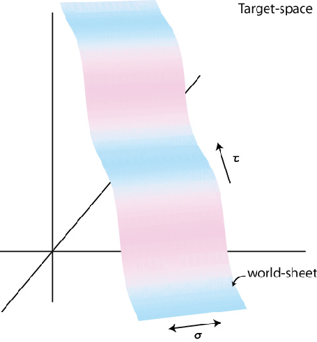
Superstring theories describe a string moving in a ten-dimensional space called the target-space. A propagating string in the target-space sweeps out a two-dimensional surface which is called the world-sheet. It can be parameterized by two parameters σ,τ\sigma,\tau. The σ\sigma-variable is the coordinate parameterizing the spatial extension along the string whereas τ\tau corresponds to the time direction, see figure 1.1. The vibrations of superstrings can have bosonic and fermionic degrees of freedom, related to each other by supersymmetry transformations. Such string theories are said to have world-sheet supersymmetry. In addition, one can consider a string which propagates in a target-space that is a superspace (it has both bosonic and fermionic coordinates). The supersymmetric structure originating in this way is called target-space supersymmetry.
Refer to caption
Figure 1.1: The world-sheet of an open string.

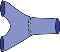
There are two coupling constants in string theory, called the string tension gg and string coupling gsg_{s}. The string tension gg describes the energy per unit length of the string and the string coupling gsg_{s} governs the splitting and joining processes of strings. When gs=0g_{s}=0 there is no string splitting/joining and the world sheet of a closed string is just a cylinder.
Refer to caption
Figure 1.2: Schematic representation of a joining/splitting process of closed strings. Any such process is weighted with the coupling constant gsg_{s}

An fascinating new insight in the dynamics of strings and strongly coupled gauge theories came with the advent of the AdS/CFT correspondence [3]. The correspondence states a duality between superstring theories of closed strings and conformal field theories. It assumes that a string theory in an anti-de Sitter (AdS) target-space is equivalent to a conformal field theory (CFT) on the conformal boundary of this space. What is remarkable about this conjecture is that it relates closed strings, which are inherently related to gravity, to a quantum field theory that has no gravitational degrees of freedom at all. In this way it provides a realization of a profound duality between open and closed strings.

We will now continue with describing the conjecture in more detail by considering the prototype example of the AdS/CFT correspondence:

𝒩=4\mathcal{N}=4 super Yang-Mills ⇔\Leftrightarrow Type IIB AdS5×S5{\rm AdS}_{5}\times{\rm S}^{5} superstring.

The AdS5×S5{\rm AdS}_{5}\times{\rm S}^{5} superstring is the string theory in a special curved target space, which is the product of the five-dimensional anti-de Sitter space AdS5{\rm AdS}_{5} and the five-dimensional sphere S5{\rm S}^{5}, see figure 1.3. The AdS5{\rm AdS}_{5} space is a maximally symmetric, five-dimensional space with negative constant curvature. It can be viewed as a hyperboloid embedded in flat space, described by the equation X02+X52−∑i=14Xi2=1X_{0}^{2}+X_{5}^{2}-\sum_{i=1}^{4}X_{i}^{2}=1.

Refer to caption
Figure 1.3: The AdS5×S5{\rm AdS}_{5}\times{\rm S}^{5} space.

According to the AdS/CFT correspondence, the string coupling constant gsg_{s} and the string tension gg are related to the 𝒩=4\mathcal{N}=4 SYM parameters, λ,N\lambda,N as

gs=λ/4​π​N,\displaystyle g_{s}=\lambda/4\pi N, g=λ/2​π.\displaystyle g=\sqrt{\lambda}/2\pi. (1.5)

The correspondence also relates gauge invariant operators of 𝒩=4\mathcal{N}=4 SYM to string states. The scaling dimensions Δ\Delta of these operators are mapped to the energies EE of corresponding string states

Δ=E.\displaystyle\Delta=E.

In other words, the spectrum of string energies should be equal to the spectrum of scaling dimensions of 𝒩=4\mathcal{N}=4 SYM. The problem of computing both spectra is naturally called the spectral problem.

The AdS/CFT correspondence is a strong-weak duality. This means that it relates the strongly coupled regime of field theories to the weakly coupled regime of the corresponding string theory and vice versa. As such, it enables to probe the strongly coupled regime of field theories via weakly-interacting strings, giving access to important strongly coupled phenomena in gauge theories. This potentially provides a direct way for string theory to have concrete applications, albeit more as a computational tool rather than as a fundamental model.

The strong-weak duality, however, is a two-edged sword. It offers truly exciting possibilities, yet it also presents a challenge in understanding the precise nature of the relation between strings and gauge theories. The reason is obvious; if one wishes to perform computations on both sides of the duality and compare the results, then generically one of the two sides will be strongly coupled and hence hard to solve. However, it turns out that both 𝒩=4\mathcal{N}=4 SYM and the AdS5×S5{\rm AdS}_{5}\times{\rm S}^{5} superstring exhibit a rich hidden symmetry structure that allows to circumvent this problem. Namely, in the planar limit both 𝒩=4\mathcal{N}=4 super Yang-Mills and the AdS5×S5{\rm AdS}_{5}\times{\rm S}^{5} superstring are described by integrable models. Integrable models are dynamical systems that have an infinite number of conservation laws, which normally imply the existence of an exact solution. One can therefore try to expand and generalize the methods and tools developed in the theory of integrable models, like for instance the Bethe ansatz, to explore and understand this prototype example at the quantitative level.

Thus, through the gauge/string correspondence, integrability offers the unprecedented possibility to completely solve, at least in the planar limit, a non-trivial quantum field theory in four dimensions. Understanding this prototype example would elucidate underlying physical mechanisms and would provide a solid basis to move on to other, more interesting, phenomenological models.

Integrability and its implementation for the AdS5×S5{\rm AdS}_{5}\times{\rm S}^{5} superstring at the quantum level is by no means straightforward. The world-sheet theory turns out to be a two-dimensional non-relativistic quantum field theory in finite volume. Standard techniques appear to be insufficient for solving this theory and therefore new methods have to be invented. One of the most recent developments in this direction is the generalization of the so-called Thermodynamic Bethe Ansatz for the AdS5×S5{\rm AdS}_{5}\times{\rm S}^{5} mirror model.

In the remainder of this chapter we will first discuss the emergence of integrability in both 𝒩=4\mathcal{N}=4 SYM and the AdS5×S5{\rm AdS}_{5}\times{\rm S}^{5} superstring. Subsequently we will elaborate on how one can use integrability techniques to find a complete solution of the spectral problem. We close this presentation by giving an outline of this review and the new results achieved.

1.1 Integrability in 𝒩=4\mathcal{N}=4 Super Yang-Mills Theory

The constituents of the 𝒩=4\mathcal{N}=4 SYM theory are: six scalar fields Φi\Phi_{i}, one vector field AμA_{\mu} and four fermions Ψ\Psi. The action is given by:

S=1gY​M2​∫d4​x​{14​(Fμ​ν)2+12​(Dμ​Φi)2−14​[Φi,Φj]2+fermions}.\displaystyle S=\frac{1}{g_{YM}^{2}}\int d^{4}x~\left\{\frac{1}{4}(F_{\mu\nu})^{2}+\frac{1}{2}(D_{\mu}\Phi_{i})^{2}-\frac{1}{4}[\Phi_{i},\Phi_{j}]^{2}+{\mathrm{fermions}}\right\}. (1.6)

The fields are in the adjoint representation of S​U​(N)SU(N), thus under a local transformation U⁡(x)∈S​U​(N)U(x)\in SU(N) they transform as

𝒳→U​𝒳​U−1,\displaystyle\mathcal{X}\rightarrow U\mathcal{X}U^{-1}, Aμ→U​Aμ​U−1−i⁡(∂μU)​U−1,\displaystyle A_{\mu}\rightarrow UA_{\mu}U^{-1}-i(\partial_{\mu}U)U^{-1}, (1.7)

where 𝒳={Φi,Ψ,Fμ​ν}\mathcal{X}=\{\Phi_{i},\Psi,F_{\mu\nu}\}. We are interested in gauge invariant composite operators. They are formed by taking the trace over products of various fields 𝒳\mathcal{X}, for instance

𝒪⁡(x)=tr⁡(…​Φi​(x)​…​Ψk​(x)​Dμ​Φj​(x)​…​Fμ​ν​(x)​…).\displaystyle\mathcal{O}(x)=\mathrm{tr}(\ldots\Phi_{i}(x)\ldots\Psi^{k}(x)D_{\mu}\Phi_{j}(x)\ldots F_{\mu\nu}(x)\ldots). (1.8)

The symmetry algebra of 𝒩=4\mathcal{N}=4 SYM includes the conformal algebra 𝔰​𝔬​(2,4)∼𝔰​𝔲​(2,2)\mathfrak{so}(2,4)\sim\mathfrak{su}(2,2) which consists of the Poincaré algebra together with conformal boosts and dilatation. Adding the supersymmetry transformations extends the conformal algebra to the superconformal algebra 𝔭​𝔰​𝔲​(2,2|4)\mathfrak{psu}(2,2|4). This is the full symmetry algebra of 𝒩=4\mathcal{N}=4 SYM.

A conformal field theory is characterized by the set of primary operators {𝒪i}\{\mathcal{O}_{i}\}. These operators correspond to highest weight states, i.e. they are annihilated by conformal boosts and conformal supercharges of the superconformal algebra. Primary operators are eigenstates of the dilatation operator 𝒟\mathcal{D}, which is one of the generators of the conformal algebra 𝔭​𝔰​𝔲​(2,2|4)\mathfrak{psu}(2,2|4)

𝒟​𝒪n=i​Δn​𝒪n.\displaystyle\mathcal{D}\mathcal{O}_{n}=i\Delta_{n}\mathcal{O}_{n}. (1.9)

In case these operators are scalar fields, one finds that their two-point function is of the form

⟨𝒪i​(x)​𝒪j​(y)⟩=δi​j|x−y|2​Δi.\displaystyle\langle\mathcal{O}_{i}(x)\mathcal{O}_{j}(y)\rangle=\frac{\delta_{ij}}{|x-y|^{2\Delta_{i}}}. (1.10)

Thus, the spectrum of scaling dimensions can be determined either by finding eigenvalues of the dilatation operator or by computing the corresponding two-point functions.

Concerning the computation of two-point functions, one finds that generically the operators 𝒪i\mathcal{O}_{i} loose their tree-level orthogonality as soon as the leading quantum correction is taken into account. This can be understood as the appearance of a non-trivial mixing

⟨𝒪i​(x)​𝒪j​(y)⟩=1|x−y|2​Δc​l​a​s​s​i​c​a​l​(δi​j+λ​Mi​j​ln⁡(|μ⁡(x−y)|)+…),\displaystyle\langle\mathcal{O}_{i}(x)\mathcal{O}_{j}(y)\rangle=\frac{1}{|x-y|^{2\Delta_{classical}}}(\delta_{ij}+\lambda M_{ij}\ln(|\mu(x-y)|)+\ldots), (1.11)

where μ\mu is a mass scale and Mi​jM_{ij} is called mixing matrix. The spectrum of conformal dimensions is then found by re-diagonalizing the basis of operators. This procedure effectively introduces a dependence of the scaling dimension on the ’t Hooft coupling Δ=Δ⁡(λ,N)\Delta=\Delta(\lambda,N).

In the planar limit, a remarkable simplification happens. The dilatation operator can be identified with a spin chain Hamiltonian, while composite gauge invariant operators are then naturally interpreted as states of this spin chain [4, 5, 6, 7, 8].

Refer to caption
Figure 1.4: Operators correspond to states on a spin chain. The fields correspond to lattice sites. The scaling dimensions Δ\Delta are identified with eigenvalues of a Hamiltonian ℋ\mathcal{H}

To exemplify this, let us restrict to scalar fields at the one-loop level. One can make the identification

tr⁡(Φi1​(x)​…​ΦiJ​(x))⟶|Φ1⟩⊗…⊗|ΦJ⟩,\displaystyle\mathrm{tr}(\Phi_{i_{1}}(x)\ldots\Phi_{i_{J}}(x))\longrightarrow|\Phi_{1}\rangle\otimes\ldots\otimes|\Phi_{J}\rangle, (1.12)

which is a state of a 𝔰​𝔬​(6)\mathfrak{so}(6) spin chain (the indices of the scalar fields transform under this algebra) with JJ sites. Cyclicity of the trace is then equivalent to the spin chain being closed.

By explicitly computing one-loop diagrams, one can show that the dilatation operator acts on neighboring fields only; it is of the form

𝒟1−loop=∑i=1JHi,i+1.\displaystyle\mathcal{D}_{1-{\rm loop}}=\sum_{i=1}^{J}H_{i,i+1}. (1.13)

This dilatation operator can be recognized as an integrable Hamiltonian of the 𝔰​𝔬​(6)\mathfrak{so}(6) spin chain. Finding scaling dimensions thus reduces to computing the eigenvalues of this integrable spin chain Hamiltonian (figure 1.4). From the gauge theory point of view, the ground state of the Hamiltonian corresponds to

tr⁡(𝒵J),\displaystyle\qquad{\rm tr}(\mathcal{Z}^{J}), 𝒵≡Φm+i​Φn,\displaystyle\mathcal{Z}\equiv\Phi_{m}+i\Phi_{n}, (1.14)

for some n,m=1,…,6n,m=1,\ldots,6. This operator is known as half-BPS, which means that it is annihilated by half of the Poincaré supercharges. As a consequence of the superconformal algebra, its scaling dimension is Δ=J\Delta=J and it is not affected by quantum corrections.

1.2 String model and integrability

The action of the AdS5×S5{\rm AdS}_{5}\times{\rm S}^{5} superstring string is of the form [9]

S=−g2∫dτdσgμ​ν(x)∂αxμ∂αxν+fermions,\displaystyle S=-\frac{g}{2}\int d\tau d\sigma~g_{\mu\nu}(x)\partial^{\alpha}x^{\mu}\partial_{\alpha}x^{\nu}+{\rm fermions}, α=σ,τ\displaystyle\alpha=\sigma,\tau

where gi​jg_{ij} is the metric of the AdS5×S5{\rm AdS}_{5}\times{\rm S}^{5} space. Let (t,zi)(t,z^{i}) be the coordinates of AdS5{\rm AdS}_{5} and (ϕ,yi)(\phi,y^{i}) the coordinates of S5{\rm S}^{5}, then it is given by

d​s2=gt​t​d​t2+gϕ​ϕ​d​ϕ2+gy​y​d​yi​d​yi+gz​z​d​zi​d​zi,\displaystyle ds^{2}=g_{tt}dt^{2}+g_{\phi\phi}d\phi^{2}+g_{yy}dy^{i}dy^{i}+g_{zz}dz^{i}dz^{i}, (1.15)

with

gt​t=(4+z24−z2)2,\displaystyle g_{tt}=\left(\frac{4+z^{2}}{4-z^{2}}\right)^{2}, gϕ​ϕ=(4−y24+y2)2,\displaystyle g_{\phi\phi}=\left(\frac{4-y^{2}}{4+y^{2}}\right)^{2}, gy​y=1(1+y24)2,\displaystyle g_{yy}=\frac{1}{(1+\frac{y^{2}}{4})^{2}}, gz​z=1(1−z24)2,\displaystyle g_{zz}=\frac{1}{(1-\frac{z^{2}}{4})^{2}}, (1.16)

where y2=yi​yiy^{2}=y^{i}y^{i} and z2=zi​ziz^{2}=z^{i}z^{i}. It is easily seen that the metric gi​jg_{ij} has isometries corresponding to shifts along the time direction tt of the AdS space and to shifts along the big circle ϕ\phi of the sphere. These correspond to global symmetries of the string model. The associated Noether charges are the energy EE of the string and its angular momentum JJ respectively.

It is useful to note that we can write both AdS5{\rm AdS}_{5} and S5{\rm S}^{5} as cosets of Lie groups:

AdS5=SO⁡(4,2)SO⁡(4,1),\displaystyle{\rm AdS}_{5}=\frac{{\rm SO(4,2)}}{{\rm SO(4,1)}}, S5=SO⁡(6)SO⁡(5).\displaystyle{\rm S}^{5}=\frac{{\rm SO(6)}}{{\rm SO(5)}}. (1.17)

More precisely, the supergroup PSU⁡(2,2|4)\mathrm{PSU}(2,2|4) contains SU⁡(2,2)×SU⁡(4)\mathrm{SU}(2,2)\times\mathrm{SU}(4) as a bosonic subgroup which is locally isomorphic to SO⁡(4,2)×SO⁡(6)\mathrm{SO}(4,2)\times\mathrm{SO}(6) . Modding PSU⁡(2,2|4)\mathrm{PSU}(2,2|4) out by SO⁡(4,1)×SO⁡(5)\mathrm{SO}(4,1)\times\mathrm{SO}(5) then gives a supersymmetric space with AdS5×S5{\rm AdS}_{5}\times{\rm S}^{5} as bosonic part. This is then a natural target-space for the AdS5×S5{\rm AdS}_{5}\times{\rm S}^{5} superstring and indeed, the superstring on AdS5×S5{\rm AdS}_{5}\times{\rm S}^{5} can be described on the coset [9]

PSU⁡(2,2|4)SO⁡(4,1)×SO⁡(5),\displaystyle\frac{\mathrm{PSU}(2,2|4)}{\mathrm{SO}(4,1)\times\mathrm{SO}(5)},

see also [10] for an extensive review. One advantage of this formulation is that it makes the global 𝔭​𝔰​𝔲​(2,2|4)\mathfrak{psu}(2,2|4) symmetry manifest. Notice that 𝔭​𝔰​𝔲​(2,2|4)\mathfrak{psu}(2,2|4) is also the symmetry algebra of 𝒩=4\mathcal{N}=4 SYM.

One can prove that, classically, the string equations of motion admit a so-called Lax representation [11]. This property implies the existence of an infinite number of conservation laws. In other words, the AdS5×S5{\rm AdS}_{5}\times{\rm S}^{5} superstring is classically integrable. The Lax representation allows one to explicitly construct the corresponding conserved charges [12] and find the solutions to the string equations of motion [13].

However, one ultimately is interested in the determination of the full quantum spectrum. At the quantum level, the 1+11+1 dimensional quantum field theory on the world-sheet also shows signs of being integrable. The spectrum of spinning strings is compatible with the assumption of integrability [14, 15, 16, 17, 18, 19, 20, 21, 22, 23, 24, 25, 26, 27, 28, 29, 30] and scattering data of world-sheet excitations also seems to exhibit the properties of integrable theories [31, 32, 33]. From now on we will assume full quantum integrability of the model and try to understand its consequences. A necessary check of this assumption is that all data that has been derived assuming integrability is in complete agreement with explicit computations.

To find the spectrum of quantum integrable field theories, one can employ the S-matrix approach, which proved to work well for many known integrable models. In the context of the AdS/CFT correspondence this approach was initiated in [34]. The AdS/CFT S-matrix and its symmetries constitute one of the main topics of this review. Below we will discuss a possible route one can undertake to find the string spectrum with the help of the S-matrix approach.

1.3 Large volume spectrum from symmetry

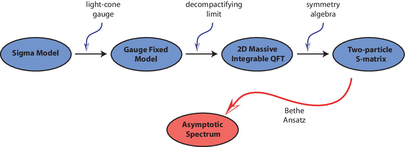
Integrability allows one to find the complete solution of the ‘large volume’ spectrum. On the gauge theory side this spectrum describes the scaling dimensions of operators composed of a large number of fields. On the string theory side, this gives the energy spectrum when the spatial size of the world-sheet goes to infinity. The S-matrix will play a crucial role in the derivation of the spectrum. How one obtains the spectrum is depicted in figure 1.5 and in what follows we will elaborate on the different steps.
Refer to caption
Figure 1.5: Road map for the asymptotic spectrum. For the gauge fixed model one finds in the infinite volume limit a massive integrable field theory. This theory has centrally extended 𝔰​𝔲​(2|2)\mathfrak{su}(2|2) as symmetry algebra. The S-matrix can be found by requiring compatibility with this algebra and is then used to find the spectrum via the Bethe ansatz.

Symmetries

The energy of the string corresponds to the Noether charge associated with the time direction in the AdS space. It turns out that it can be related to a world-sheet Hamiltonian. This reduces the problem of finding the string energy to solving a spectral problem in a two-dimensional quantum field theory.

To see how this comes about, one works in the Hamiltonian formalism. We introduce the conjugate momenta pip_{i} to a variable xix^{i}

pi=δ​Sδ⁡(∂τxi).\displaystyle p_{i}=\frac{\delta S}{\delta(\partial_{\tau}x^{i})}. (1.18)

Consider the time direction tt in the anti-de Sitter space and the angle ϕ\phi describing one of the big circles of S5S^{5}. The associated conserved charges EE and JJ can be written in terms of the conjugate momenta

E∼∫−rrd​σ​pt,\displaystyle E\sim\int_{-r}^{r}d\sigma~p_{t}, J∼∫−rrd​σ​pϕ,\displaystyle J\sim\int_{-r}^{r}d\sigma~p_{\phi}, (1.19)

where we take the string world-sheet to be of size −r≤σ≤r-r\leq\sigma\leq r.

To remove the non-physical degrees of freedom one imposes the so-called the light-cone gauge [35, 36, 37]. To this end, we define the light-cone coordinates

x−=ϕ−t,\displaystyle x_{-}=\phi-t, x+=t,\displaystyle x_{+}=t, p−=pϕ+pt,\displaystyle p_{-}=p_{\phi}+p_{t}, p+=pϕ,\displaystyle p_{+}=p_{\phi}, (1.20)

In these coordinates, the conserved charges can be expressed as follows

P−∼∫−rrd​σ​p−=J−E,\displaystyle P_{-}\sim\int_{-r}^{r}d\sigma p_{-}=J-E, P+∼∫−rrd​σ​p+=J.\displaystyle P_{+}\sim\int_{-r}^{r}d\sigma p_{+}=J. (1.21)

The light-cone gauge is now imposed by setting

x+=τ,\displaystyle x_{+}=\tau, p+=1,\displaystyle p_{+}=1, (1.22)

from which it follows that r∼P+=Jr\sim P_{+}=J. In other words, the size of the world-sheet is proportional to the angular momentum of the string. To find the complete gauge fixed action, one solves the Virasoro constraints which give the light-cone momentum in terms of the transverse coordinates p−​(xi,x′i)p_{-}(x^{i},x^{\prime i}). The world-sheet Hamiltonian density is given by

ℋ=−p−​(xi,x′i).\displaystyle\mathcal{H}=-p_{-}(x^{i},x^{\prime i}). (1.23)

The world-sheet Hamiltonian is then related to the string energy and angular momentum via

H=∫−rrd​σ​ℋ=E−J.\displaystyle H=\int_{-r}^{r}d\sigma\mathcal{H}=E-J. (1.24)

Here one sees that the space-time energy EE of the string is directly related to the spectrum of the world-sheet Hamiltonian HH in this gauge. This means that one can find the spectrum of the superstring (and hence the spectrum of scaling dimensions of the dual four-dimensional field theory) by solving the spectral problem of the two-dimensional world-sheet theory.

For closed strings, periodicity of the fields implies that the total world-sheet momentum pp defined by

p≡−∫−rrdσpi∂σxi\displaystyle p\equiv-\int_{-r}^{r}d\sigma~p_{i}\partial_{\sigma}x^{i} (1.25)

has to vanish. This condition is referred to as the level-matching condition. States that satisfy this condition are called on-shell and states with non-vanishing momentum are called off-shell. The level-matching condition can not be solved explicitly for the fields, but it needs to be imposed on physical states in the theory. One then proceeds by studying the off-shell theory, keeping in mind that for physical states the level-matching needs to be imposed at the end.

The next step is to consider the limit P+→∞P_{+}\rightarrow\infty while keeping the string tension gg fixed. In this limit, the world-sheet theory becomes a massive field theory defined on a plane. Because of this, asymptotic states and the S-matrix are well-defined. The gauged superstring has eight bosonic fields and eight fermionic fields.

Refer to caption
Figure 1.6: In the infinite volume limit theory is defined on a plane.

The gauge-fixing string model still has some residual symmetry left. It turns out that the 𝔭​𝔰​𝔲​(2,2|4)\mathfrak{psu}(2,2|4) algebra from the coset model is reduced to two copies of 𝔭​𝔰​𝔲​(2|2)\mathfrak{psu}(2|2)11 1 The same algebra also appears on the field theory side [38]. [39]. For the off-shell theory this symmetry algebra gets extended and becomes two copies of centrally extended 𝔰​𝔲​(2|2)\mathfrak{su}(2|2). More precisely, the 1616 degrees of freedom (88 bosons and 88 fermions)

8B+8F=16=4×4.\displaystyle 8_{B}+8_{F}=16=4\times 4. (1.26)

transform under the tensor product of two fundamental representations of centrally extended 𝔰​𝔲​(2|2)\mathfrak{su}(2|2). This fundamental representation is four dimensional and is spanned by two bosonic and two fermionic basis vectors.

The centrally extended 𝔰​𝔲​(2|2)\mathfrak{su}(2|2) Lie superalgebra consists of two copies of 𝔰​𝔲​(2)\mathfrak{su}(2), whose generators we denote by 𝕃,ℝ{\mathbb{L}},{\mathbb{R}} together with two sets of supersymmetry generators ℚ,ℚ†{\mathbb{Q}},{\mathbb{Q}}^{{\dagger}}. The non-trivial commutation relations are given by

[𝕃ab,𝕁c]=δcb​𝕁a−12​δab​𝕁c\displaystyle[\mathbb{L}_{a}^{b},\mathbb{J}_{c}]=\delta_{c}^{b}\mathbb{J}_{a}-\frac{1}{2}\delta_{a}^{b}\mathbb{J}_{c} [ℝαβ,𝕁γ]=δγβ​𝕁α−12​δαβ​𝕁γ\displaystyle[\mathbb{R}_{\alpha}^{\beta},\mathbb{J}_{\gamma}]=\delta_{\gamma}^{\beta}\mathbb{J}_{\alpha}-\frac{1}{2}\delta_{\alpha}^{\beta}\mathbb{J}_{\gamma}
[𝕃ab,𝕁c]=−δac​𝕁b+12​δab​𝕁c\displaystyle[\mathbb{L}_{a}^{b},\mathbb{J}^{c}]=-\delta_{a}^{c}\mathbb{J}^{b}+\frac{1}{2}\delta_{a}^{b}\mathbb{J}^{c} [ℝαβ,𝕁γ]=−δαγ​𝕁β+12​δαβ​𝕁γ\displaystyle[\mathbb{R}_{\alpha}^{\beta},\mathbb{J}^{\gamma}]=-\delta^{\gamma}_{\alpha}\mathbb{J}^{\beta}+\frac{1}{2}\delta_{\alpha}^{\beta}\mathbb{J}^{\gamma} (1.27)
{ℚαa,ℚβb}=ϵα​β​ϵa​b​ℂ\displaystyle\{\mathbb{Q}_{\alpha}^{a},\mathbb{Q}_{\beta}^{b}\}=\epsilon_{\alpha\beta}\epsilon^{ab}\mathbb{C} {ℚa†α,ℚb†β}=ϵα​β​ϵa​b​ℂ†\displaystyle\{\mathbb{Q}^{{\dagger}\alpha}_{a},\mathbb{Q}^{{\dagger}\beta}_{b}\}=\epsilon^{\alpha\beta}\epsilon_{ab}\mathbb{C}^{{\dagger}}
{ℚαa,ℚb†β}=δba​ℝαβ+δαβ​𝕃ba+12​δba​δαβ​ℍ,\displaystyle\{\mathbb{Q}_{\alpha}^{a},\mathbb{Q}^{{\dagger}\beta}_{b}\}=\delta_{b}^{a}\mathbb{R}_{\alpha}^{\beta}+\delta_{\alpha}^{\beta}\mathbb{L}_{b}^{a}+\frac{1}{2}\delta_{b}^{a}\delta_{\alpha}^{\beta}\mathbb{H},

where 𝕁\mathbb{J} stands for any generator with appropriate index structure. The central extensions ℂ,ℂ†{\mathbb{C}},{\mathbb{C}}^{{\dagger}} make the anti-commutator between the supercharges non-zero. The central charges are related to the world-sheet momentum pp and the string tension gg as

ℂ=i​g2​(ei​p−1),\displaystyle\mathbb{C}=\frac{ig}{2}(e^{ip}-1), ℂ†=−i​g2​(e−i​p−1).\displaystyle\mathbb{C}^{{\dagger}}=-\frac{ig}{2}(e^{-ip}-1). (1.28)

For on-shell configurations these central charges vanish.

Scattering

The existence of an infinite number of conservation laws greatly restricts scattering in an integrable theory. More precisely, scattering processes in integrable quantum field theories exhibit the following properties

  • •

    Absence of particle production and annihilation

  • •

    Conservation of the sets of initial and final momenta

  • •

    Factorization of multi-particle scattering into a sequence of two-body scattering events

  • •

    The two-body S-matrix satisfies a consistency condition which deals with equivalent orderings of scattering of multi-particle states called the Yang-Baxter equation.

These properties imply that, in integrable models, the two-body S-matrix is the fundamental building block of the scattering theory.

Having identified the symmetry properties of the gauge-fixed action, we should find its implications for scattering processes. The S-matrix relates i​nin-eigenstates to o​u​tout-eigenstates of the Hamiltonian and it should be compatible with the symmetry of the underlying model. This means that any such scattering matrix 𝕊{\mathbb{S}} should commute with the action of any symmetry generator 𝕁\mathbb{J}

𝕊​𝕁=𝕁​𝕊.\displaystyle{\mathbb{S}}~\mathbb{J}=\mathbb{J}~{\mathbb{S}}. (1.29)

This is schematically depicted in figure 1.7. The action of the symmetry generators on the in- and out-states are encoded in a structure called the coproduct. The coproduct is an operation in Hopf algebras which naturally encodes the action of symmetry generators on two-particle states. Since each of the world-sheet excitations transforms in a sixteen dimensional representation, the S-matrix will be a 256×256256\times 256 dimensional matrix.

Refer to caption
Figure 1.7: Symmetry commutes with scattering.

The remarkable fact is that requiring the two-body S-matrix for fundamental excitations to respect centrally extended 𝔰​𝔲​(2|2)\mathfrak{su}(2|2) is enough to fix it up to an overall scalar factor S0S_{0} [38, 40]. For its explicit form we refer to equation (4.1), but it can be shown that it satisfies all physical properties associated with integrable field theories

Unitarity:

𝕊12​𝕊21=𝟙\qquad\,\,\,\,\,\,\,\,\,\,\,\,{\mathbb{S}}_{12}{\mathbb{S}}_{21}=\mathbbm{1}.

Hermiticity:

𝕊12​𝕊12†=𝟙\,\,\,\,\,\,\qquad{\mathbb{S}}_{12}{\mathbb{S}}_{12}^{{\dagger}}=\mathbbm{1}.

CPT Invariance:

𝕊12=𝕊12t\,\,\,\,{\mathbb{S}}_{12}={\mathbb{S}}_{12}^{t}.

Yang-Baxter Equation:

𝕊12​𝕊13​𝕊23=𝕊23​𝕊13​𝕊12\,\,\,\qquad{\mathbb{S}}_{12}{\mathbb{S}}_{13}{\mathbb{S}}_{23}={\mathbb{S}}_{23}{\mathbb{S}}_{13}{\mathbb{S}}_{12}.

Based on the additional requirement of crossing symmetry [41], the overall scalar factor has also been conjectured [42, 43, 44] and was found to agree with all known computations so far.

Concluding, the expression for the full S-matrix is conjectured relying heavily on its symmetry properties. It is an exact quantity in the coupling gg and hence interpolates between strong and weak coupling.

Large volume spectrum

In integrable models one usually can derive the exact large volume spectrum from the S-matrix by a technique called the Bethe Ansatz. This technique dates back to 1931, where it was first used to solve the Heisenberg XXX-spin chain [45]. Over the years this technique has been cast into many different forms and it has found its way into various physical models.

The Bethe Ansatz offers a method to capture the spectrum of an integrable Hamiltonian in a set of algebraic equations, called the Bethe ansatz equations. This is done by making a plane-wave type ansatz for the eigenstates of the Hamiltonian. This ansatz depends on a set of momenta which are restricted by imposing periodic boundary conditions. This is similar, for example, to a free particle on a circle of circumference LL for which periodic boundary conditions ei​p​L=1e^{ipL}=1 imply that the momentum is quantized. The reason periodicity needs to be imposed is that even though we consider the theory on the plane, it still comes from a closed string, i.e. a cylindric world-sheet. How to impose periodicity has a very clear interpretation.

Refer to caption
Figure 1.8: Periodicity is imposed by scattering a particle along the line.

Consider NN particles with momenta pip_{i} on a line with length LL. If we take one particle and move it along the line, it will scatter on its way with all the other particles via the two-body S-matrix. However, when it has travelled a distance LL, it returns back at its original position and the state should remain unchanged, up to a phase factor ei​p1​Le^{ip_{1}L}, which is due to the plane-wave type ansatz. If we denote the S-matrix with SS, then the Bethe equations are of the form

ei​pj​L=∏i≠jS⁡(pi,pj).\displaystyle e^{ip_{j}L}=\prod_{i\neq j}S(p_{i},p_{j}). (1.30)

This can be seen as a quantization condition on the momenta. The spectrum is then obtained by first solving the Bethe equations for the set of momenta {pi}\{p_{i}\}, which can then be substituted in the Hamiltonian. The dispersion relation for the AdS5×S5{\rm AdS}_{5}\times{\rm S}^{5} superstring is known in terms of the momenta pp and is given by [46]

H=1+4​g2​sin2⁡p2.\displaystyle H=\sqrt{1+4g^{2}\sin^{2}\frac{p}{2}}. (1.31)

The total energy of the state is obtained by summing the contributions of the particles

Ht​o​t=∑iH⁡(pi).\displaystyle H_{tot}=\sum_{i}H(p_{i}). (1.32)

The above discussion depends crucially on the two-particle S-matrix of the theory. Since this matrix is known for the AdS5×S5{\rm AdS}_{5}\times{\rm S}^{5} superstring (in the large volume limit) to all orders in the coupling gg, the spectrum obtained in this way is also exact.

The situation for the AdS5×S5{\rm AdS}_{5}\times{\rm S}^{5} superstring appears to be more complicated than presented above. The S-matrix has a non-trivial matrix structure which mixes particles of different types. This can be taken into account by extending the Bethe ansatz resulting in a so-called nested structure. The Bethe equations were found in [38, 47] and further investigated in [48, 49]. They are given by

ei​pk​L\displaystyle e^{ip_{k}L} =\displaystyle= ∏l=1,l≠kKI[S0​(pk,pl)​xk+−xl−xk−−xl+​xl+​xk−xl−​xk+]2​∏α=12∏l=1K(α)IIxk−−yl(α)xk+−yl(α)​xk+xk−\displaystyle\prod_{l=1,l\neq k}^{K^{\mathrm{I}}}\left[S_{0}(p_{k},p_{l})\frac{x_{k}^{+}-x_{l}^{-}}{x_{k}^{-}-x_{l}^{+}}\sqrt{\frac{x_{l}^{+}x_{k}^{-}}{x_{l}^{-}x_{k}^{+}}}\right]^{2}\prod_{\alpha=1}^{2}\prod_{l=1}^{K_{(\alpha)}^{\mathrm{II}}}\frac{{x_{k}^{-}-y^{(\alpha)}_{l}}}{x_{k}^{+}-y^{(\alpha)}_{l}}\sqrt{\frac{x^{+}_{k}}{x^{-}_{k}}}
1\displaystyle 1 =\displaystyle= ∏l=1KIyk(α)−xl+yk(α)−xl−​xk−xk+​∏l=1K(α)IIIyk(α)+1yk(α)−wl(α)+igyk(α)+1yk(α)−wl(α)−ig\displaystyle\prod_{l=1}^{K^{\mathrm{I}}}\frac{y^{(\alpha)}_{k}-x^{+}_{l}}{y^{(\alpha)}_{k}-x^{-}_{l}}\sqrt{\frac{x^{-}_{k}}{x^{+}_{k}}}\prod_{l=1}^{K_{(\alpha)}^{\mathrm{III}}}\frac{y_{k}^{(\alpha)}+\frac{1}{y_{k}^{(\alpha)}}-w_{l}^{(\alpha)}+\frac{i}{g}}{y_{k}^{(\alpha)}+\frac{1}{y_{k}^{(\alpha)}}-w_{l}^{(\alpha)}-\frac{i}{g}} (1.33)
1\displaystyle 1 =\displaystyle= ∏l=1K(α)IIwk(α)−yk(α)−1yk(α)+igwk(α)−yk(α)−1yk(α)−ig​∏l≠kK(α)IIIwk(α)−wl(α)−2​igwk(α)−wlα+2​ig,\displaystyle\prod_{l=1}^{K_{(\alpha)}^{\mathrm{II}}}\frac{w_{k}^{(\alpha)}-y_{k}^{(\alpha)}-\frac{1}{y_{k}^{(\alpha)}}+\frac{i}{g}}{w_{k}^{(\alpha)}-y_{k}^{(\alpha)}-\frac{1}{y_{k}^{(\alpha)}}-\frac{i}{g}}\prod_{l\neq k}^{K_{(\alpha)}^{\mathrm{III}}}\frac{w_{k}^{(\alpha)}-w_{l}^{(\alpha)}-\frac{2i}{g}}{w_{k}^{(\alpha)}-w_{l}^{\alpha}+\frac{2i}{g}},

where α=1,2\alpha=1,2 reflect the two copies of 𝔰​𝔲​(2|2)\mathfrak{su}(2|2) and S0​(pk,pl)S_{0}(p_{k},p_{l}) is the overall scalar factor of the S-matrix. The parameters x±x^{\pm} are related to the coupling gg and to the world-sheet momentum via22 2 A similar parameterization also appears in the Hubbard model.

x++1x+−x−−1x−=2​ig,\displaystyle x^{+}+\frac{1}{x^{+}}-x^{-}-\frac{1}{x^{-}}=\frac{2i}{g}, x+x−=ei​p.\displaystyle\frac{x^{+}}{x^{-}}=e^{ip}. (1.34)

The parameters yi,wiy_{i},w_{i} are auxiliary variables that one introduces to deal with the matrix structure of the S-matrix. The spectrum is then again found by solving this coupled set of equations and plugging the solution in the dispersion relation (1.31).

Because one can only define the scattering theory on the infinite plane, these Bethe equations only encompass the asymptotic part of the spectrum. The big remaining challenge is then to compute the spectrum for finite size world-sheets.

Emergence of bound states

Before addressing the finite size problem, let us first take a closer look at the Bethe equations and discuss the emergence of bound states. Bound states are composite particles which belong to the physical spectrum and which manifest themselves as poles of a multi-particle S-matrix, see for example [50, 51]. It was found that the fundamental particles of the AdS5×S5{\rm AdS}_{5}\times{\rm S}^{5} superstring model can indeed form bound states [52, 53, 54, 55, 56]. They transform in symmetric short representations of centrally extended 𝔰​𝔲​(2|2)\mathfrak{su}(2|2) [55], which are discussed in chapter 3.

Consider two particles with complex momenta p1=p2−i​qp_{1}=\frac{p}{2}-iq and p2=p2+i​qp_{2}=\frac{p}{2}+iq, with pp real and Re​q>0\mathrm{Re}~q>0. It is easy to see that in the large volume limit ei​p1​Je^{ip_{1}J} tends to ∞\infty. When looking at the first line of the Bethe equations (1.33) we see that such a solution can indeed exist if the right hand side exhibits a pole

x−​(p1)−x+​(p2)=0,\displaystyle x^{-}(p_{1})-x^{+}(p_{2})=0, (1.35)

which corresponds to a pole in the S-matrix. The above relation implies a non-trivial equation for p,qp,q. From (1.35) one can show that the total energy becomes

H=H⁡(p1)+H⁡(p2)=22+4​g2​sin2⁡p2.\displaystyle H=H(p_{1})+H(p_{2})=\sqrt{2^{2}+4g^{2}\sin^{2}\frac{p}{2}}. (1.36)

This discussion generalizes to multi-particle bound states. The latter are composites of ℓ\ell fundamental particles whose momenta are related by the condition

x−​(pi)−x+​(pi+1)=0.\displaystyle x^{-}(p_{i})-x^{+}(p_{i+1})=0. (1.37)

The energy of these bound state particles is given by the dispersion relation

H=ℓ2+4​g2​sin2⁡p2.\displaystyle H=\sqrt{\ell^{2}+4g^{2}\sin^{2}\frac{p}{2}}. (1.38)

A bound state that consists of ℓ\ell fundamental particles and transforms in a short representation of centrally extended 𝔰​𝔲​(2|2)\mathfrak{su}(2|2) which is 4​ℓ4\ell dimensional. Concluding, the complete asymptotic spectrum consists of fundamental excitations and their bound states.

1.4 Towards finite size

To deal with the finite-size spectral problem, two approaches have been developed in the past in the context of relativistic models. One of them is a perturbative approach due to Lüscher [57] and the other is the Thermodynamic Bethe Ansatz (TBA) [58, 59]. Both approaches have been recently extended to account for the unconventional structure of the AdS5×S5{\rm AdS}_{5}\times{\rm S}^{5} string model.

Lüscher’s perturbative approach

In [57] the leading finite-size correction to energies were computed using diagrammatic methods. This formalism has been adapted to the AdS5×S5{\rm AdS}_{5}\times{\rm S}^{5} superstring [60, 61, 62, 63, 64, 65]. The idea is that, in compact spaces, particle energies pick up corrections coming from virtual particles moving around the compact direction, see figure 1.9. Where the particle meets the virtual particle from the loop they scatter via the S-matrix. The virtual particles that run in the loop can be both fundamental or bound state.

Refer to caption
Figure 1.9: Diagrams for finite-size systems. The dashed line depicts a virtual particle moving around the compact direction.

The first successful application of this procedure was the computation of the four-loop scaling dimension of the Konishi operator in 𝒩=4\mathcal{N}=4 SYM. The Konishi operator is of the form

K=tr⁡(D​𝒵​D​𝒵)−tr⁡(𝒵​D2​𝒵),\displaystyle K={\rm tr}(D\mathcal{Z}D\mathcal{Z})-{\rm tr}(\mathcal{Z}D^{2}\mathcal{Z}), (1.39)

where D=D1+i​D2D=D_{1}+iD_{2}. One can compute its scaling dimension directly in field theory [66, 67, 68]. It gives

ΔK=4+3​g2−3​g4+214​g6+[−394+9​ζ​(3)4−45​ζ​(5)8]​g8.\displaystyle\Delta_{K}=4+3g^{2}-3g^{4}+\frac{21}{4}g^{6}+\left[-\frac{39}{4}+\frac{9\zeta(3)}{4}-\frac{45\zeta(5)}{8}\right]g^{8}. (1.40)

To derive this result one has to take into account around 200 supergraphs or equivalently 130000 Feynman diagrams. Needless to say, these are complicated and demanding computations. However, this result can also be derived from string theory in a very simple and elegant way, as we will explain below.

First, one has to identify the string state to which the Konishi operator corresponds. On the string theory side, KK corresponds to the state built up out of two world-sheet excitations corresponding to the light-cone derivatives DD, with momenta p1,p2p_{1},p_{2}. The level-matching condition implies that p=p1=−p2p=p_{1}=-p_{2}. The angular momentum of the string is found to be J=2J=2. From the Bethe equations (1.33) one can solve perturbatively for the momentum pp to find

p=2​π3−34​g2+9​332​g4+….\displaystyle p=\frac{2\pi}{3}-\frac{\sqrt{3}}{4}g^{2}+\frac{9\sqrt{3}}{32}g^{4}+\ldots. (1.41)

From this momentum, one can then compute the energy via the dispersion relation (1.31)

EB​A​E=J+H=4+1+4​g2​sin2⁡p12+1+4​g2​sin2⁡p22.\displaystyle E_{BAE}=J+H=4+\sqrt{1+4g^{2}\sin^{2}\frac{p_{1}}{2}}+\sqrt{1+4g^{2}\sin^{2}\frac{p_{2}}{2}}. (1.42)

The field theory computation is done in perturbation theory at weak coupling, so in order to compare with this, one expands the energy EB​A​EE_{BAE} around g=0g=0 and finds

EB​A​E=4+3​g2−3​g4+214​g6+[−70564+9​ζ​(3)8]​g8.\displaystyle E_{BAE}=4+3g^{2}-3g^{4}+\frac{21}{4}g^{6}+\left[-\frac{705}{64}+\frac{9\zeta(3)}{8}\right]g^{8}. (1.43)

We see a disagreement in the g8g^{8} term. However, it turns out that the Lüscher correction exactly contributes to this term. Indeed, when the Lüscher correction is taken into account, one does find perfect agreement [63]

EB​A​E+L=4+3​g2−3​g4+214​g6+[394+9​ζ​(3)4−45​ζ​(5)8]​g8.\displaystyle E_{BAE+L}=4+3g^{2}-3g^{4}+\frac{21}{4}g^{6}+\left[\frac{39}{4}+\frac{9\zeta(3)}{4}-\frac{45\zeta(5)}{8}\right]g^{8}. (1.44)

Summarizing, by using the Bethe ansatz for the string model supplemented by the leading Lüscher correction, one finds beautiful agreement with the result of a highly non-trivial quantum field theory computation.

Although generating these nice results, Lüscher’s approach is perturbative in nature and, therefore, has its limitations. The problem of establishing the exact spectrum is further addressed by the TBA approach, to which Lüscher’s technique can be seen as a certain approximation. The regions of the (g,J)(g,J)-parameter plane where the various techniques to study the string/gauge theory spectrum are applicable are schematically depicted in figure 1.10. The TBA should cover the entire diagram.

Refer to caption
Figure 1.10: Overview of the known parts of the spectrum. The coupling constant gg runs along the vertical axis and the size of the system on the horizontal. In the weak coupling regime perturbative gauge theory computations are possible and in the strong coupling regime one can perform perturbative string computations. For infinite sizes one can compute the asymptotic spectrum via Bethe ansatz techniques. The TBA should provide a complete covering of the diagram.

Thermodynamic Bethe Ansatz

The TBA approach in the AdS/CFT spectral problem was first advocated in [60] where it was used to explain wrapping effects in gauge theory. We will follow [56] where the first results towards an explicit construction of the corresponding TBA approach were obtained.

Consider the world-sheet of a closed string which is parameterized by variables σ\sigma and τ\tau. In the thermodynamic Bethe ansatz (TBA) approach one considers a closed string of size LL which wraps a ‘time’-loop of size RR. In this way one makes the time variable τ\tau periodic. The surface that is formed in this way is a torus; the product of two circles of circumferences L,RL,R, see figure 1.11.

Refer to caption
Figure 1.11: String model and mirror model both come from the same torus. They are related via a double Wick rotation.

By performing a Wick rotation τ→i​τ\tau\rightarrow i\tau one obtains an Euclidean theory associated with this torus. In this Euclidean theory there is no distinction between the coordinates and because of this, one can associate two different ‘Minkowski’ models to this theory, namely one can apply an inverse Wick rotation to both variables.

Applying the inverse Wick rotation to the τ\tau variable inevitably returns us back to the string model we started out with. Applying it to the σ\sigma variable, however, gives a new model, called ‘mirror’ model. This mirror model is then related to the original string model via a double Wick rotation

σ~=−i​τ,\displaystyle\tilde{\sigma}=-i\tau, τ~=i​σ.\displaystyle\tilde{\tau}=i\sigma. (1.45)

Notice that the roles of position and time are interchanged. Consequently, the mirror model also has a different Hamiltonian H~\tilde{H}, which is now defined with respect to τ~\tilde{\tau}.

It turns out that the mirror theory is different from the world-sheet theory of the AdS5×S5{\rm AdS}_{5}\times{\rm S}^{5} superstring. For example, the dispersion relation is now given by

H~=2​a​r​c​s​i​n​h​1+p~22​g,\displaystyle\tilde{H}=2\mathrm{arcsinh}\frac{\sqrt{1+\tilde{p}^{2}}}{2g}, (1.46)

where p~\tilde{p} is the momentum of the mirror particles, cf. (1.31). Nevertheless, one can show that the partition functions Z​(R,L),Z~​(L,R)Z(R,L),\tilde{Z}(L,R) of both models are equal. They are given by

Z⁡(R,L)≡∑n⟨ψn|e−H​R|ψn⟩=∑ne−En​R\displaystyle Z(R,L)\equiv\sum_{n}\langle\psi_{n}|e^{-HR}|\psi_{n}\rangle=\sum_{n}e^{-E_{n}R} (1.47)
Z~​(L,R)≡∑n⟨ψ~n|e−H~​L|ψ~n⟩.\displaystyle\tilde{Z}(L,R)\equiv\sum_{n}\langle\tilde{\psi}_{n}|e^{-\tilde{H}L}|\tilde{\psi}_{n}\rangle. (1.48)

In the limit R→∞R\rightarrow\infty one obtains

log⁡Z⁡(R,L)⟶R→∞−R​E​(L),\displaystyle\log Z(R,L)\stackrel{{\scriptstyle R\rightarrow\infty}}{{\longrightarrow}}-RE(L), log⁡Z~​(R,L)⟶R→∞−R​L​f​(L),\displaystyle\log\tilde{Z}(R,L)\stackrel{{\scriptstyle R\rightarrow\infty}}{{\longrightarrow}}-RLf(L), (1.49)

where E⁡(L)E(L) is the ground state energy and f⁡(L)f(L) is the free energy per unit length of the mirror model at temperature 1/L1/L. Since both partition functions agree, one finds

E⁡(L)=L​f​(L).\displaystyle E(L)=Lf(L). (1.50)

We see that by sending R→∞R\rightarrow\infty, the ground state energy of the AdS5×S5{\rm AdS}_{5}\times{\rm S}^{5} superstring in finite volume LL is described by the free energy of the mirror theory in infinite volume but at finite temperature 1/L1/L. This is the basic idea of the TBA; the spectrum of the original theory can be computed through thermodynamic quantities in the mirror model.

The importance of these observations is that, for the mirror model, one can still use all the large volume techniques that have been described earlier to compute the exact spectrum. In fact, the mirror model in the infinite volume limit also exhibits centrally extended 𝔰​𝔲​(2|2)\mathfrak{su}(2|2) symmetry. This means that the same symmetry arguments are applicable to the large volume spectrum for the mirror model. Finally, one has to work at finite temperature and identify all states that contribute in the thermodynamic limit [69].

In the mirror theory, the S-matrix again contains poles that correspond to bound states [56]. In other words, the complete asymptotic spectrum is composed of fundamental particles and their bound states. More precisely, this means that bound states will contribute in the thermodynamic limit. Because of this, their scattering data and spectrum needs to be understood.

The thermodynamic limit is implemented by sending R→∞R\rightarrow\infty while keeping Ni/RN_{i}/R fixed, where NiN_{i} is the number of particles of a certain species ii. From the Bethe equations that describe the large volume spectrum, one can then derive the TBA equations which constitute an infinite number of coupled integral equations. These equations are supposed to describe the finite-size spectrum of the original string theory [70, 71, 70, 72]. The TBA approach perfectly accommodates Lüscher’s correction, which emerges from the large JJ asymptotic solutions of the TBA equations for excited states. The future challenge is to obtain a detailed understanding of the TBA solutions. The first results in this direction are very promising [73, 74, 75, 76, 77, 78, 79]. The agreement between the TBA approach and Lüscher’s approach has even been extended to the five-loop level [65, 80, 81, 82].

1.5 Bound States and Yangian

Bound states and their scattering data play an important role in both the TBA and in Lüscher’s perturbative approach. The S-matrix for fundamental representations was fixed by the requirement that it respects the 𝔰​𝔲​(2|2)\mathfrak{su}(2|2) symmetry. One might wonder whether similar symmetry arguments can also be applied to bound states.

Bound states of fundamental particles transform in higher dimensional representations of centrally extended 𝔰​𝔲​(2|2)\mathfrak{su}(2|2). Because of this, it turns out that invariance under the extended 𝔰​𝔲​(2|2)\mathfrak{su}(2|2) algebra is no longer enough to fix the matrix structure for these higher dimensional representations [83, 84]. In addition, one has to invoke the Yang-Baxter equation to completely fix the S-matrix. However, it was shown that the fundamental S-matrix is actually invariant under a bigger symmetry group; the Yangian of 𝔰​𝔲​(2|2)\mathfrak{su}(2|2) [83].

The Yangian of a Lie algebra can be seen as an infinite dimensional deformation of the associated loop algebra. Consider an algebra with structure constants fCA​Bf^{AB}_{C}

[𝕁A,𝕁B]=fCA​B​𝕁C\displaystyle[\mathbb{J}^{A},\mathbb{J}^{B}]=f^{AB}_{C}\mathbb{J}^{C}

and introduce a new set of generators 𝕁^A\hat{\mathbb{J}}^{A} that satisfy the relation

[𝕁A,𝕁^B]=fCA​B​𝕁^C.\displaystyle[\mathbb{J}^{A},\hat{\mathbb{J}}^{B}]=f^{AB}_{C}\hat{\mathbb{J}}^{C}.

The Yangian of the algebra is now spanned by the generators 𝕁A,𝕁^A\mathbb{J}^{A},\hat{\mathbb{J}}^{A} and commutators thereof, generating an infinite dimensional algebra. It turns out that bound state S-matrices are fixed by requiring invariance under the Yangian of centrally extended 𝔰​𝔲​(2|2)\mathfrak{su}(2|2) rather than only the algebra itself [85]. In fact, one can construct any bound state S-matrix by using Yangian symmetry33 3 Similarly, (Yangian) symmetry is also crucial in finding boundary S-matrices for open strings, see e.g. [86, 87]. [88].

1.6 Different models

The main focus here is on the AdS5×S5{\rm AdS}_{5}\times{\rm S}^{5} superstring and its partner 𝒩=4\mathcal{N}=4 super Yang-Mills. One might wonder how useful this is for physical applications since 𝒩=4\mathcal{N}=4 SYM is a rather special quantum field theory. It is conformal and highly supersymmetric, properties that are not shared with real-world theories like QCD. Nevertheless, one can smoothly deform the AdS5×S5{\rm AdS}_{5}\times{\rm S}^{5} space-time [89] to obtain a deformed 𝒩=1\mathcal{N}=1 SYM theory. Even though the number of supersymmetries is reduced, one still finds integrable structures [90, 91, 92]. One might hope to apply the TBA approach to this case as well. There even exists a more general class of deformations [93] which is expected to be dual to a non-supersymmetric gauge theory. A thorough understanding of the prime example which is central in this work can then, via these related models, be used to extend our understanding of the AdS/CFT correspondence to more realistic models.

A different example of a pair of dual theories is [94]

𝒩=6\mathcal{N}=6 Chern-Simons Theory ↔\leftrightarrow IIA strings on AdS4×ℂ​ℙ3{\rm AdS}_{4}\times\mathbb{CP}^{3}.

It also admits a formulation in terms of a coset model [95, 96] and one can show that the model is classically integrable. The asymptotic symmetry is again centrally extended 𝔰​𝔲​(2|2)\mathfrak{su}(2|2) and, because of this, it has many features in common with the AdS5×S5{\rm AdS}_{5}\times{\rm S}^{5} superstring and its partner 𝒩=4\mathcal{N}=4 SYM. Also for this model the asymptotic Bethe equations have been proposed [97] and the set of TBA equations have recently been conjectured [98, 99]. Even though there are quite some similarities between this instance of the AdS/CFT correspondence and the prototype example, there are also differences. Elucidating those can provide a partial guide to what new features could be expected on the way towards understanding more realistic models.

The importance of a complete understanding of the aforementioned theories goes beyond giving evidence for the AdS/CFT correspondence. On the one hand, the integrable structures can allow for a determination of the complete spectrum of 𝒩=4\mathcal{N}=4 SYM. This would then be the first exact solution of a non-trivial four-dimensional quantum field theory. On the other hand, a comprehensive description of the corresponding string model could prove invaluable in the future. A full solution might serve as a benchmark against which future computational methods in string theory can be checked and refined.

1.7 Outline

In this chapter we outlined a very promising road that hopefully leads to a full determination of the spectrum of the AdS5×S5{\rm AdS}_{5}\times{\rm S}^{5} superstring and through the AdS/CFT correspondence to the spectrum of scaling dimensions of 𝒩=4\mathcal{N}=4 SYM. The material in this review particulary focusses on two aspects that were encountered along this way, namely scattering data of bound states and the Bethe ansatz.

First, the S-matrix describing the scattering of bound states with arbitrary bound state numbers is explicitly constructed by using Yangian symmetry, see equations (4.76),(4.105),(4.121). We study its classical limit and compare it against two different proposals in the literature [100, 101], finding agreement only with the latter. We also examine some of its mathematical features. More precisely we find blocks in this S-matrix that exhibit universal algebraic properties.

The next topic is the computation of the large volume spectrum of bound state configurations. The fact that we explicitly know the S-matrix allows us to apply the Bethe ansatz and impose periodic boundary conditions. This results in a set of Bethe equations that describe the large volume bound state spectrum (7.98). We have also found an alternative way to derive these equations by using the underlying Yangian symmetry of the S-matrix. These Bethe equations play a crucial role in the derivation of the TBA equations. A second approach that we have examined is that of the algebraic Bethe ansatz. We present the explicit transfer matrices (8.56), from which one, once again, can derive the Bethe equations. The algebraic Bethe ansatz is also a useful framework for possible future investigations like form factors.

This remainder of this review is organized as follows. In chapter 2, we will first give a brief introduction to integrable models and Hopf algebras. In this chapter we also introduce the notion of a Yangian.

After this we will discuss in chapter 3 the algebra that plays a key role in the whole discussion: centrally extended 𝔰​𝔲​(2|2)\mathfrak{su}(2|2). We will give its defining relations and discuss in detail the representations describing both fundamental particles and their bound states. Subsequently, we introduce the Hopf algebra structure that is used to derive the S-matrix. We finish the chapter with a discussion of the Yangian of 𝔰​𝔲​(2|2)\mathfrak{su}(2|2), which is important for the determination of the bound state scattering data.

In chapter 4 the bound state S-matrix will be derived by making use of Yangian symmetry. Using the two 𝔰​𝔲​(2)\mathfrak{su}(2) subalgebras contained in 𝔰​𝔲​(2|2)\mathfrak{su}(2|2) one can split states into three different types. We first solve for one specific type of states (equation (4.76)) and then, via the different supersymmetry generators, extend the solution to the whole space, (equations (4.105) and (4.121)). This results in an explicit formula for the bound state scattering data that agrees with all S-matrices that were previously found.

Since the underlying algebra determines the entire scattering data, one might wonder whether it can be written purely in algebraic terms. Such an algebraic object corresponding to the S-matrix is called a universal R-matrix in the framework of Hopf algebras. This is the subject of chapters 5 and 6. In the first chapter the classical limit of the bound state S-matrix is studied and one finds agreement with a universal expression that has been proposed in the literature. In the subsequent chapter we study certain blocks in the S-matrix that exhibit universality at the full quantum level.

After this more mathematically oriented part we move on to the determination of the spectrum. We will first do this by applying the coordinate Bethe ansatz. After a discussion of this technique applied to the non-linear Schrödinger model we will introduce nesting to deal with particles with different colors and generalize the discussion to the AdS5×S5{\rm AdS}_{5}\times{\rm S}^{5} superstring. This Bethe ansatz procedure can then be reformulated by making use of the Yangian symmetry, which allows for a derivation of the Bethe equations describing the asymptotic bound state spectrum [102].

Alternatively one can use the algebraic Bethe ansatz, which is done in chapter 8. In this approach one derives the eigenvalues of the transfer matrix, that play a crucial role in the TBA. We will derive an explicit expression for the eigenvalues of the transfer matrix for generic bound state representations (8.56). Some of these eigenvalues were already conjectured in the literature [55] via a fusion procedure. We work this procedure out explicitly and compare it to our results, finding perfect agreement.

Chapter 2 Integrable Models and Hopf Algebras

The notion of integrability was already briefly touched upon in the introduction. In this chapter we will expand this discussion. We will particulary focus on the relation between integrability and Hopf algebras. The mathematical language of Hopf algebras is useful in describing symmetries of integrable field theories and we will use it frequently.

We will first briefly discuss the notion of integrability in classical mechanics and in the theory of partial differential equations. We then continue with an overview of scattering processes in integrable field theories and introduce the notion of Hopf algebras and Yangians. After this we will show in an example how Yangians can arise in an integrable theory.

2.1 Classical Integrable Systems

Examples of classical integrable systems can be encountered e.g. when solving problems of Newtonian mechanics. Most of such problems, like Kepler’s one, are well-known. However exact solutions, especially when dealing with multiple degrees of freedom, are rather rare. In the 19th century Liouville derived a theorem in which a big class of exactly solvable models was identified, the so-called integrable models. For an extensive treatment on this topic we refer to [103].

Finite-Dimensional Integrable Models

Consider a system with Hamiltonian ℋ\mathcal{H}, coordinates qiq_{i} and conjugate momenta pip_{i}. Its equations of motion are written as

q˙i=∂ℋ∂pi,\displaystyle\dot{q}_{i}=\frac{\partial\mathcal{H}}{\partial p_{i}}, p˙i=−∂ℋ∂qi.\displaystyle\dot{p}_{i}=-\frac{\partial\mathcal{H}}{\partial q_{i}}. (2.1)

The time evolution of any quantity F⁡(p,q)F(p,q) is given by

F˙={ℋ,F},\displaystyle\dot{F}=\{\mathcal{H},F\}, (2.2)

where {,}\{,\} is the Poisson bracket. Suppose that the phase space is 2​N2N dimensional. The system is called integrable if there are NN (functionally) independent conserved quantities FiF_{i} (of which the Hamiltonian is one), which mutually Poisson commute

{Fi,Fj}=0,\displaystyle\{F_{i},F_{j}\}=0, {Fi,ℋ}=0,for​all​i,j.\displaystyle\{F_{i},\mathcal{H}\}=0,\qquad\mathrm{for\ all\ }i,j. (2.3)

Liouville’s theorem states that an integrable system can be solved by quadratures, i.e. by solving a finite number of algebraic equations and computing a finite number of integrals. In this sense integrable models are exactly solvable.

Examples of integrable systems include the harmonic oscillator (the conserved quantity is the Hamiltonian F=ℋF=\mathcal{H}) and Kepler’s problem (conserved quantities are the Hamiltonian, the total angular momentum and the z-component of the angular momentum: F1=ℋ,F2=J3,F3=J2F_{1}=\mathcal{H},F_{2}=J_{3},F_{3}=J^{2}).

A different way to formulate integrability is in terms of a so-called Lax pair. Suppose there are matrices L⁡(p,q),M⁡(p,q)L(p,q),M(p,q) such that one can write the equations of motion in the following way

∂0L−[L,M]=0.\displaystyle\partial_{0}L-[L,M]=0. (2.4)

(From now on we denote the time derivative as ∂0\partial_{0} rather then using a dot). If this is the case, then one can straightforwardly see that the quantities

Ik=tr​Lk\displaystyle I_{k}={\rm{tr}}L^{k} (2.5)

are conserved. The property that these quantities Poisson commute it related to an object called classical rr-matrix. Assuming one can prove that these quantities are independent and Poisson commute with one another, we see that such a system is integrable.

The harmonic oscillator admits a Lax-pair. Define the matrices

L=(pω​qω​q−p),\displaystyle L=\begin{pmatrix}p&\omega q\\ \omega q&-p\end{pmatrix}, M=(0−ω2ω20).\displaystyle M=\begin{pmatrix}0&-\frac{\omega}{2}\\ \frac{\omega}{2}&0\end{pmatrix}.\ (2.6)

Then one can readily check that these indeed encode the equations of motion in the form (2.4). The Hamiltonian is given by ℋ=14​tr​L2\mathcal{H}=\frac{1}{4}{\rm{tr}}L^{2}.

Since conserved charges correspond to symmetries via Noether’s theorem, one finds that integrable models have enough symmetries to be solved by quadratures.

Integrable Partial Differential Equations

There is a related notion of integrability for two-dimensional (non-linear) partial differential equations (PDE). These equations admit a reformulation analogous to the Lax pair one discussed above.

Let Ψ⁡(t,x,z)\Psi(t,x,z) be a rank nn vector, and consider the overdetermined set of equations

∂0Ψ⁡(t,x,z)=L0​(t,x,z)​Ψ​(t,x,z),\displaystyle\partial_{0}\Psi(t,x,z)=L_{0}(t,x,z)\Psi(t,x,z), ∂1Ψ⁡(t,x,z)=L1​(t,x,z)​Ψ​(t,x,z),\displaystyle\partial_{1}\Psi(t,x,z)=L_{1}(t,x,z)\Psi(t,x,z), (2.7)

where ∂1=∂x\partial_{1}=\partial_{x} and Li​(t,x,z)L_{i}(t,x,z) are n×nn\times n matrices. By considering the double derivative ∂0∂1Ψ⁡(t,x,z)=∂1∂0Ψ⁡(t,x,z)\partial_{0}\partial_{1}\Psi(t,x,z)=\partial_{1}\partial_{0}\Psi(t,x,z) one sees that the matrices Li​(t,x,z)L_{i}(t,x,z) need to satisfy the consistency condition

∂0L1−∂1L0+[L1,L0]=0.\displaystyle\partial_{0}L_{1}-\partial_{1}L_{0}+[L_{1},L_{0}]=0. (2.8)

The above equation can be seen as the flatness condition for a two-dimensional (non-abelian) connection. This connection is called the Lax connection and it is a generalization of the notion of a Lax pair (2.4).

If a PDE can be written as the flatness condition for a Lax connection, then it is called integrable. For example, the sine-Gordon equation

ϕt​t−ϕx​x+m2β​sin⁡(β​ϕ)=0,\displaystyle\phi_{tt}-\phi_{xx}+\frac{m^{2}}{\beta}\sin(\beta\phi)=0, (2.9)

can be written in this way via the following Lax connection:

L1=β​ϕt4​i​(100−1)+k0​sin⁡β​ϕ2i​(0110)+k1​cos⁡β​ϕ2i​(0−ii0)\displaystyle L_{1}=\frac{\beta\phi_{t}}{4i}\begin{pmatrix}1&0\\ 0&-1\end{pmatrix}+\frac{k_{0}\sin\frac{\beta\phi}{2}}{i}\begin{pmatrix}0&1\\ 1&0\end{pmatrix}+\frac{k_{1}\cos\frac{\beta\phi}{2}}{i}\begin{pmatrix}0&-i\\ i&0\end{pmatrix} (2.10)
L0=β​ϕx4​i​(100−1)+k1​sin⁡β​ϕ2i​(0110)+k0​cos⁡β​ϕ2i​(0−ii0)\displaystyle L_{0}=\frac{\beta\phi_{x}}{4i}\begin{pmatrix}1&0\\ 0&-1\end{pmatrix}+\frac{k_{1}\sin\frac{\beta\phi}{2}}{i}\begin{pmatrix}0&1\\ 1&0\end{pmatrix}+\frac{k_{0}\cos\frac{\beta\phi}{2}}{i}\begin{pmatrix}0&-i\\ i&0\end{pmatrix} (2.11)

with

k0=m4​(z+1z),\displaystyle k_{0}=\frac{m}{4}\left(z+\frac{1}{z}\right), k1=m4​(z−1z).\displaystyle k_{1}=\frac{m}{4}\left(z-\frac{1}{z}\right). (2.12)

From a Lax connection one can construct an infinite tower of conserved charges. In this case this can be achieved by defining a monodromy matrix T⁡(z)T(z) as the path ordered exponential of the Lax connection. Expanding this quantity in the parameter zz then generates the conserved quantities [103].

2.2 Integrable 2d Relativistic Field Theories

The notion of integrability can be extended to two dimensional quantum field theories. Also in these theories, integrability corresponds to the system having an enhanced symmetry resulting in an infinite set of conservation laws. This is translated into the fact that scattering processes in these theories have very special features. The scattering processes have the following properties [104, 105, 51]

Absence of Particle Production

There is no particle production in these systems.

[Uncaptioned image]
Momentum Conservation

The sets of initial and final momenta are the same

{pi}i​n={pi}o​u​t.\displaystyle\{p_{i}\}_{in}=\{p_{i}\}_{out}. (2.13)
Factorizability

Any scattering process reduces to a chain of two-body interactions

(n→n)=∏(2→2).\displaystyle(n\rightarrow n)~~=~~\prod~(2\rightarrow 2). (2.14)
Unitarity
[Uncaptioned image]
𝕊12​(p1,p2)​𝕊21​(p2,p1)=𝟙.\displaystyle{\mathbb{S}}_{12}(p_{1},p_{2}){\mathbb{S}}_{21}(p_{2},p_{1})=\mathbbm{1}. (2.15)
Crossing

Scattering is symmetric under particle to anti-particle transformations

[Uncaptioned image]
𝕊12​(p1,p2)=𝕊2¯​1​(p1,p2~)\displaystyle{\mathbb{S}}_{12}(p_{1},p_{2})={\mathbb{S}}_{\bar{2}1}(p_{1},\tilde{p_{2}}) (2.16)
Yang-Baxter Equation

The two body S-matrix satisfies a consistency condition which can be derived by considering the factorization of three particle scattering.

[Uncaptioned image]
𝕊12​𝕊13​𝕊23=𝕊23​𝕊13​𝕊12.\displaystyle{\mathbb{S}}_{12}{\mathbb{S}}_{13}{\mathbb{S}}_{23}={\mathbb{S}}_{23}{\mathbb{S}}_{13}{\mathbb{S}}_{12}. (2.17)

One can often take the above set of conditions as a definition of an integrable (quantum) field theory. Examples of such a theories are for instance the Sine-Gordon model [106] and the Sinh-Gordon model [51].

From the factorization property we see that all scattering information in such theories is encoded in the two-body S-matrix. This means that computing this scattering process is the key to solving these systems.

2.3 Hopf Algebras

A convenient mathematical framework to deal with symmetries of integrable models is the language of Hopf algebras. Hopf algebras carry with them the structure of a coproduct and an antipode. From the physical point of view the coproduct describes the action of symmetry generators on multi-particle states and the antipode corresponds to a particle to anti-particle transformation.

We will review basic facts and definitions of Hopf algebras. We will be mostly interested in those associated to Lie (super)algebras. A very special family of Hopf algebras are the Yangians. These are infinite dimensional algebras associated to Lie algebras. They appear as symmetry algebras in various integrable models and are important in our understanding of the spectrum of the AdS5×S5{\rm AdS}_{5}\times{\rm S}^{5} superstring.

There is a vast literature on this subject and for a more detailed analysis of Yangians and Hopf algebras we refer to [107, 108, 109, 110, 111, 112, 113, 114].

Definitions

An associative algebra AA with unit is a vector space over ℂ\mathbb{C} (the notion of algebra is more general, but will restrict to complex vector spaces) that is equipped with a multiplication μ\mu

μ:A⊗A→A,a1⊗a2→μ⁡(a1⊗a2)≡a1​a2.\displaystyle\mu:A\otimes A\rightarrow A,\qquad a_{1}\otimes a_{2}\rightarrow\mu(a_{1}\otimes a_{2})\equiv a_{1}a_{2}. (2.18)

and a unit under multiplication η:ℂ→A\eta:\mathbb{C}\rightarrow A, such that

μ⁡(η⁡(λ)⊗a)=λ​a=μ⁡(a⊗η⁡(λ)),\displaystyle\mu(\eta(\lambda)\otimes a)=\lambda a=\mu(a\otimes\eta(\lambda)), λ∈ℂ,a∈A.\displaystyle\lambda\in\mathbb{C},a\in A. (2.19)

The multiplication is bilinear and associativity is formulated as

a⁡(b​c)=(a​b)​c,a,b,c∈A.\displaystyle a(bc)=(ab)c,\qquad a,b,c\in A. (2.20)

An obvious example of a such an algebra is the vector space of n×nn\times n complex matrices with the standard matrix multiplication and η⁡(λ)=λ​𝟙\eta(\lambda)=\lambda\mathbbm{1}. Let 𝒫:A⊗A→A⊗A\mathcal{P}:A\otimes A\rightarrow A\otimes A be the (graded) permutation operator, then we say that the algebra is commutative if μ∘𝒫=μ\mu\circ\mathcal{P}=\mu.

A coalgebra AA is an object which has a structure ‘dual’ to that of an algebra; it has a comultiplication Δ\Delta and a co-unit ϵ\epsilon

Δ:A→A⊗A,\displaystyle\Delta:A\rightarrow A\otimes A, ϵ:A→ℂ.\displaystyle\epsilon:A\rightarrow\mathbb{C}. (2.21)

Similarly these maps have to be bilinear and the coproduct needs to satisfy coassociativity

(Δ⊗𝟙)​Δ=(𝟙⊗Δ)​Δ.\displaystyle(\Delta\otimes\mathbbm{1})\Delta=(\mathbbm{1}\otimes\Delta)\Delta. (2.22)

A coalgebra is called cocommutative if 𝒫​Δ=Δ\mathcal{P}\Delta=\Delta. We call Δo​p=𝒫​Δ\Delta^{op}=\mathcal{P}\Delta the opposite coproduct.

An algebra AA is called a bialgebra if it also is endowed with the structure of a coalgebra such that Δ\Delta and ϵ\epsilon are algebra homomorphisms, i.e. they respect the multiplicative structure

Δ⁡(a1​a2)=Δ⁡(a1)⋅Δ⁡(a2),\displaystyle\Delta(a_{1}a_{2})=\Delta(a_{1})\cdot\Delta(a_{2}), ϵ⁡(a1​a2)=ϵ⁡(a1)​ϵ​(a2),\displaystyle\epsilon(a_{1}a_{2})=\epsilon(a_{1})\epsilon(a_{2}), (2.23)
ϵ⁡(𝟙)=1,\displaystyle\epsilon(\mathbbm{1})=1, Δ​𝟙=𝟙⊗𝟙.\displaystyle\Delta\mathbbm{1}=\mathbbm{1}\otimes\mathbbm{1}. (2.24)

Finally a Hopf algebra HH is a bialgebra which is equipped with an anti-homomorphism called the antipode 𝒮:A→A{\cal S}:A\rightarrow A, which satisfies

𝒮⁡(a1​a2)=𝒮⁡(a2)​𝒮​(a1),\displaystyle\mathcal{S}(a_{1}a_{2})=\mathcal{S}(a_{2})\mathcal{S}(a_{1}), μ⁡(𝒮⊗𝟙)∘Δ=ϵ=μ⁡(𝟙⊗𝒮)∘Δ,\displaystyle\mu({\cal S}\otimes\mathbbm{1})\circ\Delta=\epsilon=\mu(\mathbbm{1}\otimes{\cal S})\circ\Delta, (2.25)

where in the graded case one has to pick up relevant signs due to the graded structure. The first property is what defines 𝒮\mathcal{S} to be an anti-homomorphism. An example of a Hopf algebra is the universal enveloping algebra of a Lie algebra. This algebra is automatically equipped with a multiplication, which in case of a matrix representation is just matrix multiplication. One can equip it with a Hopf algebra structure by specifying

Δ⁡(𝕁A)=𝕁A⊗𝟙+𝟙⊗𝕁A,\displaystyle\Delta(\mathbb{J}^{A})=\mathbb{J}^{A}\otimes\mathbbm{1}+\mathbbm{1}\otimes\mathbb{J}^{A}, ϵ⁡(𝕁A)=0,\displaystyle\epsilon(\mathbb{J}^{A})=0, 𝒮⁡(𝕁A)=−𝕁A,\displaystyle{\cal S}(\mathbb{J}^{A})=-\mathbb{J}^{A}, (2.26)

and one can use the homomorphism properties to extend the above maps to products of elements. It is easy to check that the maps defined in this way respect multiplication (and hence also the Lie bracket). This Hopf algebra is cocommutative, but generically not commutative as an algebra.

The coproduct offers a natural way to extend a representation of a Lie algebra 𝔤\mathfrak{g} on a vector space VV to a tensor product representation on V⊗VV\otimes V. One can use (Δ⊗𝟙)​Δ(\Delta\otimes\mathbbm{1})\Delta to define it on a triple tensor product and so on. By coassociativity one gets the same structure from using (𝟙⊗Δ)​Δ(\mathbbm{1}\otimes\Delta)\Delta.

The above definition of the coproduct for the universal enveloping algebra (2.26) is natural in the language of symmetries in physics. For example, consider two particles |m1⟩,|m2⟩|m_{1}\rangle,|m_{2}\rangle in quantum mechanics with z-component of the angular momenta m1,m2m_{1},m_{2}. One expects to find that in their tensor product state |m1⟩⊗|m2⟩|m_{1}\rangle\otimes|m_{2}\rangle their charges m1m_{1} and m2m_{2} add. The operator S^z\hat{S}_{z} is just an element of 𝔰​𝔲​(2)\mathfrak{su}(2), in other words one has

S^z(|m1⟩⊗|m2⟩)≡S^z|m1,m2⟩=(m1+m2)|m1,m2⟩=ΔSz|m1,m2⟩,\displaystyle\hat{S}_{z}(|m_{1}\rangle\otimes|m_{2}\rangle)\equiv\hat{S}_{z}|m_{1},m_{2}\rangle=(m_{1}+m_{2})|m_{1},m_{2}\rangle=\Delta S_{z}|m_{1},m_{2}\rangle, (2.27)

by the above definition of the coproduct (2.26). This indeed indicates that the coproduct encodes the natural action of symmetry generators on multi-particle states.

Quasitriangular Hopf algebras

To any Hopf algebra (H,ϵ,𝒮,Δ)(H,\epsilon,\mathcal{S},\Delta) one can associate another Hopf algebra (H,ϵ,𝒮,Δo​p)(H,\epsilon,\mathcal{S},\Delta^{op}) by equipping it with the opposite coproduct Δo​p\Delta^{op} rather than Δ\Delta. This Hopf algebra is called the opposite Hopf algebra Ho​pH^{op}.

Generically there need not be a relation between the two different Hopf algebra structures. However, there is a class of Hopf algebras called quasi-cocommutative Hopf algebras, where there is an invertible element 𝕊∈H⊗H{\mathbb{S}}\in H\otimes H such that

Δo​p​𝕁​𝕊=𝕊​Δ​𝕁,\displaystyle\Delta^{op}\mathbb{J}~{\mathbb{S}}={\mathbb{S}}~\Delta\mathbb{J}, 𝕁∈H.\displaystyle\mathbb{J}\in H. (2.28)

The element 𝕊{\mathbb{S}} is called the R-matrix in mathematics. In physics this object corresponds to the S-matrix. The motivation for this is as follows. In physics the S-matrix relates in-states to out-states of the Hamiltonian.

Refer to caption
Figure 2.1: Symmetry commutes with scattering.

For definiteness, consider an elastic scattering process of two to two particles. The in-state can then be seen as two particles with the fastest one to the left and the slowest one on the right, figure 2.1. After they scatter, the particles have changed places and the fastest one is now on the right. If the theory possesses some symmetry algebra, then the S-matrix should be compatible with this algebra. This now translates into (2.28). In the context of integrable models, this can be made more precise by using the so-called Faddeev-Zamolodchikov algebra [104, 115].

Suppose now that the R-matrix satisfies the extra conditions

(Δ⊗𝟙)​(𝕊)=𝕊13​𝕊23,\displaystyle(\Delta\otimes\mathbbm{1})({\mathbb{S}})={\mathbb{S}}_{13}{\mathbb{S}}_{23}, (𝟙⊗Δ)​(𝕊)=𝕊13​𝕊12,\displaystyle(\mathbbm{1}\otimes\Delta)({\mathbb{S}})={\mathbb{S}}_{13}{\mathbb{S}}_{12}, (2.29)

then the Hopf algebra is called quasitriangular. The R-matrix of a quasitriangular Hopf algebra satisfies the following properties

𝕊12​𝕊13​𝕊23=𝕊23​𝕊13​𝕊12,\displaystyle{\mathbb{S}}_{12}{\mathbb{S}}_{13}{\mathbb{S}}_{23}={\mathbb{S}}_{23}{\mathbb{S}}_{13}{\mathbb{S}}_{12}, (𝒮⊗𝟙)​𝕊=(𝟙⊗𝒮−1)​𝕊=𝕊−1.\displaystyle(\mathcal{S}\otimes\mathbbm{1}){\mathbb{S}}=(\mathbbm{1}\otimes\mathcal{S}^{-1}){\mathbb{S}}={\mathbb{S}}^{-1}. (2.30)

The first relation is easily recognized as the Yang-Baxter equation (2.17) and the second corresponds to the crossing equation (2.16). These equations were important properties of scattering processes in integrable field theories and they arise naturally in the context of Hopf algebras.

In the above we assumed that the R-matrix was an element of H⊗HH\otimes H, but the abstract form of this element might be hard to find. However, in a specific representation, the intertwining R-matrix can usually be computed explicitly. In what follows we will refer to the R-matrix seen as an abstract element in H⊗HH\otimes H as the universal R-matrix. The intertwining operator in an explicit representation will be referred to as the S-matrix.

2.4 Yangians

A class of Hopf algebras that play an important role in integrable systems are the so-called Yangians. The Yangians are a family of infinite dimensional algebras that are associated to Lie algebras. They are constructed by introducing an additional set of generators to the Lie algebra ones. In this section we collect some basic facts about Yangians. For more details see e.g [109, 110, 113, 114].

Definition

Consider the universal enveloping algebra U⁡(𝔤)U(\mathfrak{g}) of a (simple) Lie algebra 𝔤\mathfrak{g}, with structure constants fCA​Bf^{AB}_{C}

[𝕁A,𝕁B]=fCA​B​𝕁C.\displaystyle[\mathbb{J}^{A},\mathbb{J}^{B}]=f^{AB}_{C}\mathbb{J}^{C}. (2.31)

The Yangian Y⁡(𝔤)Y(\mathfrak{g}) of this Lie algebra is the algebra generated by the generators 𝕁\mathbb{J} of 𝔤\mathfrak{g} and a new set of generators 𝕁^\hat{\mathbb{J}}, subject to

[𝕁A,𝕁^B]=fCA​B​𝕁^C.\displaystyle[\mathbb{J}^{A},\hat{\mathbb{J}}^{B}]=f^{AB}_{C}\hat{\mathbb{J}}^{C}. (2.32)

Higher level generators can then be obtained by commuting two level one generators and so on. The above commutation relations should obey the Jacobi and Serre relations (these are for algebras other than 𝔰​𝔲​(2)\mathfrak{su}(2))

[𝕁[A,[𝕁B,𝕁C]]]=0\displaystyle\left[\mathbb{J}^{[A},[\mathbb{J}^{B},\mathbb{J}^{C]}]\right]=0
[𝕁[A,[𝕁B,𝕁^C]]]=0\displaystyle\left[\mathbb{J}^{[A},[\mathbb{J}^{B},\hat{\mathbb{J}}^{C]}]\right]=0
[𝕁^[A,[𝕁^B,𝕁C]]]=14fDA​GfEB​HfFC​KfG​H​K𝕁(DCLOSE𝕁E𝕁OPENF),\displaystyle\left[\hat{\mathbb{J}}^{[A},[\hat{\mathbb{J}}^{B},\mathbb{J}^{C]}]\right]=\frac{1}{4}f^{AG}_{D}f^{BH}_{E}f^{CK}_{F}f_{GHK}\mathbb{J}^{(D}\mathbb{J}^{E}\mathbb{J}^{F)},

where (),[](),[] in the indices stand for total symmetrization and anti-symmetrization, respectively. The indices of the structure constants are lowered with the Cartan-Killing matrix.

The Yangian can be given the structure of a Hopf algebra by specifying the following coproduct

Δ​𝕁A=𝕁A⊗𝟙+𝟙⊗𝕁A\displaystyle\Delta\mathbb{J}^{A}=\mathbb{J}^{A}\otimes\mathbbm{1}+\mathbbm{1}\otimes\mathbb{J}^{A} Δ​𝕁^A=𝕁^A⊗𝟙+𝟙⊗𝕁^A+12​fB​CA​𝕁B⊗𝕁C.\displaystyle\Delta\hat{\mathbb{J}}^{A}=\hat{\mathbb{J}}^{A}\otimes\mathbbm{1}+\mathbbm{1}\otimes\hat{\mathbb{J}}^{A}+\frac{1}{2}f_{BC}^{A}\mathbb{J}^{B}\otimes\mathbb{J}^{C}. (2.33)

The coproducts of the higher level generators are obtained by using the fact that Δ\Delta should respect commutators. Then antipode is given by

𝒮⁡(𝕁A)=−𝕁A\displaystyle{\cal S}(\mathbb{J}^{A})=-\mathbb{J}^{A} 𝒮⁡(𝕁^A)=−𝕁^A+14​fB​CA​fDB​C​𝕁D,\displaystyle{\cal S}(\hat{\mathbb{J}}^{A})=-\hat{\mathbb{J}}^{A}+\frac{1}{4}f^{A}_{BC}f^{BC}_{D}\mathbb{J}^{D}, (2.34)

and the counit is

ϵ⁡(𝕁A)=ϵ⁡(𝕁^A)=0\displaystyle\epsilon(\mathbb{J}^{A})=\epsilon(\hat{\mathbb{J}}^{A})=0 ϵ⁡(𝟙)=1.\displaystyle\epsilon(\mathbbm{1})=1. (2.35)

This realization of the Yangian is called Drinfeld’s first realization.

Drinfeld’s second realization

There is also a second realization of a Yangian. This realization turns out to be particulary useful when checking the Serre relations of a representation explicitly or in constructing the universal R-matrix [116, 117].

The second realization of the Yangian [114] is given in terms of Chevalley-Serre type generators κi,m,ξi,m±\kappa_{i,m},\xi^{\pm}_{i,m}, i=1,…,rank​𝔤i=1,\dots,\text{rank}\mathfrak{g}, m=0,1,2,…m=0,1,2,\dots satisfying relations

[κi,m,κj,n]=0,[κi,0,ξj,m+]=ai​j​ξj,m+,\displaystyle[\kappa_{i,m},\kappa_{j,n}]=0,\quad[\kappa_{i,0},\xi^{+}_{j,m}]=a_{ij}\,\xi^{+}_{j,m},
[κi,0,ξj,m−]=−ai​j​ξj,m−,[ξj,m+,ξj,n−]=δi,j​κj,n+m,\displaystyle[\kappa_{i,0},\xi^{-}_{j,m}]=-a_{ij}\,\xi^{-}_{j,m},\quad[\xi^{+}_{j,m},\xi^{-}_{j,n}]=\delta_{i,j}\,\kappa_{j,n+m},
[κi,m+1,ξj,n+]−[κi,m,ξj,n+1+]=12​ai​j​{κi,m,ξj,n+},\displaystyle[\kappa_{i,m+1},\xi^{+}_{j,n}]-[\kappa_{i,m},\xi^{+}_{j,n+1}]=\frac{1}{2}a_{ij}\{\kappa_{i,m},\xi^{+}_{j,n}\},
[κi,m+1,ξj,n−]−[κi,m,ξj,n+1−]=−12​ai​j​{κi,m,ξj,n−},\displaystyle[\kappa_{i,m+1},\xi^{-}_{j,n}]-[\kappa_{i,m},\xi^{-}_{j,n+1}]=-\frac{1}{2}a_{ij}\{\kappa_{i,m},\xi^{-}_{j,n}\},
[ξi,m+1±,ξj,n±]−[ξi,m±,ξj,n+1±]=±12​ai​j​{ξi,m±,ξj,n±},\displaystyle[\xi^{\pm}_{i,m+1},\xi^{\pm}_{j,n}]-[\xi^{\pm}_{i,m},\xi^{\pm}_{j,n+1}]=\pm\frac{1}{2}a_{ij}\{\xi^{\pm}_{i,m},\xi^{\pm}_{j,n}\},
i≠j,ni​j=1+|ai​j|,S​y​m{k}​[ξi,k1±,[ξi,k2±,…​[ξi,kni​j±,ξj,l±]​…]]=0.\displaystyle i\neq j,\,\,\,\,n_{ij}=1+|a_{ij}|,\,\,\,\,\,Sym_{\{k\}}[\xi^{\pm}_{i,k_{1}},[\xi^{\pm}_{i,k_{2}},\dots[\xi^{\pm}_{i,k_{n_{ij}}},\xi^{\pm}_{j,l}]\dots]]=0. (2.36)

In these formulas, ai​ja_{ij} is the (symmetric) Cartan matrix. The index mm in the generators is referred to as the level.

Drinfeld [114] gave an explicit isomorphism between the two realizations as follows. Let us define a Chevalley-Serre basis for 𝔤\mathfrak{g} as composed of Cartan generators ℌi\mathfrak{H}_{i}, and positive (negative) simple roots 𝔈i+\mathfrak{E}^{+}_{i} (𝔈i−\mathfrak{E}^{-}_{i}, respectively). Then one has

κi,0=ℌi,ξi,0+=𝔈i+,ξi,0−=𝔈i−,\displaystyle\kappa_{i,0}=\mathfrak{H}_{i},\quad\xi^{+}_{i,0}=\mathfrak{E}^{+}_{i},\quad\xi^{-}_{i,0}=\mathfrak{E}^{-}_{i},
κi,1=ℌ^i−vi,ξi,1+=𝔈^i+−wi,ξi,1−=𝔈^i−−zi,\displaystyle\kappa_{i,1}=\hat{\mathfrak{H}}_{i}-v_{i},\quad\xi^{+}_{i,1}=\hat{\mathfrak{E}}^{+}_{i}-w_{i},\quad\xi^{-}_{i,1}=\hat{\mathfrak{E}}^{-}_{i}-z_{i}, (2.37)

where vi,wi,ziv_{i},w_{i},z_{i} are certain quadratic combinations of level-zero generators that we will not list here explicitly. From the level-zero and level-one generators, one can then recursively construct all higher-level generators by repeated use of the relations (2.36).

We will employ both the first and second realization of the Yangian in the other chapters.

Evaluation representation

An important representation of the Yangian Y⁡(𝔤)Y(\mathfrak{g}) is the evaluation representation. Let us work in Drinfeld’s first realization. Consider a representation VV of 𝔤\mathfrak{g} and introduce a parameter uu. Then V⁡(u)V(u) can host a so-called evaluation representation of Y⁡(𝔤)Y(\mathfrak{g}) by setting

𝕁^A​|v⟩=u​𝕁A​|v⟩,\displaystyle\hat{\mathbb{J}}^{A}|v\rangle=u\,\mathbb{J}^{A}|v\rangle, |v⟩∈V.\displaystyle|v\rangle\in V. (2.38)

Of course in order for this to be a valid representation, one needs to check that the Serre relations are satisfied.

Double Yangian

The Yangian Y⁡(𝔤)Y(\mathfrak{g}) of a Lie (super)algebra is not quasitriangular, i.e. there is no element 𝕊∈Y⁡(𝔤)⊗Y⁡(𝔤){\mathbb{S}}\in Y(\mathfrak{g})\otimes Y(\mathfrak{g}) that intertwines the coproduct with the opposite coproduct. However, there exists a Hopf algebra called the double Yangian D​Y​(𝔤)DY(\mathfrak{g}) which is defined by relations (2.36) but now one takes the level m∈ℤm\in\mathbb{Z} [114, 116]. On evaluation representations this means that also negative powers of the evaluation parameter uu are considered.

This enhanced algebra is quasitriangular for simple Lie algebras [116]. For the Yangian of Lie superalgebras this is not known, although it has been found in specific cases see for instance [117, 118, 108, 119]. The Yangian Y⁡(𝔤)Y(\mathfrak{g}) can be identified with a subalgebra of D​Y​(𝔤)DY(\mathfrak{g}) by restricting to elements with positive level. This means that in any representation, the universal R-matrix of D​Y​(𝔤)DY(\mathfrak{g}) also gives the S-matrix that relates the coproduct and opposite coproduct for Y⁡(𝔤)Y(\mathfrak{g}).

2.5 Integrability and Yangians

We have already seen that the R-matrix of a quasitriangular Hopf algebra is closely related to the S-matrix of integrable systems. Yangians also appear naturally in the context of integrable models. They appear in a variety of systems like the Hubbard model [120], the XXX spin chain [121] and also, as we will see later, in the AdS5×S5{\rm AdS}_{5}\times{\rm S}^{5} superstring [83]. In this section we will treat an example of how a Yangian can arise in integrable models [109].

Consider a two-dimensional field theory with Noether currents taking values in some Lie-algebra 𝔤\mathfrak{g}

Jμ=Jμ;a​(t,x)​ta,t∈𝔤.\displaystyle J_{\mu}=J_{\mu;a}(t,x)t^{a},\qquad t\in\mathfrak{g}. (2.39)

These currents are conserved on-shell

∂μJμ=0,\displaystyle\partial^{\mu}J_{\mu}=0, (2.40)

and hence they define conserved charges

Qa=∫d​x​J0;a.\displaystyle Q_{a}=\int dxJ_{0;a}. (2.41)

Assume that the currents satisfy the flatness condition

∂0J1−∂1J0+[J0,J1]=0.\displaystyle\partial_{0}J_{1}-\partial_{1}J_{0}+[J_{0},J_{1}]=0. (2.42)

Both conservation of the current and the above condition (2.42) are equivalent to the flatness of the following Lax connection

Lμ​(t,x,z)=11−z2​(Jμ​(t,x)+z​ϵμν​Jν​(t,x)).\displaystyle L_{\mu}(t,x,z)=\frac{1}{1-z^{2}}(J_{\mu}(t,x)+z\epsilon_{\mu}^{\nu}J_{\nu}(t,x)). (2.43)

In this sense this model is integrable. An example of such a model is the principal chiral model see e.g. [122, 10]. Due to integrability one expects to find more conserved charges than just the ones corresponding to the Lie algebra. Because of the flatness condition it turns out that one can define an additional non-local current

J^μ;a​(t,x)=ϵμ​ν​Jaν​(t,x)−i2​fa​b​c​Jμ;b​(t,x)​∫−∞xd​y​J0;c​(t,x).\displaystyle\hat{J}_{\mu;a}(t,x)=\epsilon_{\mu\nu}J^{\nu}_{a}(t,x)-\frac{i}{2}f_{abc}J_{\mu;b}(t,x)\int_{-\infty}^{x}dyJ_{0;c}(t,x). (2.44)

One can then show that the corresponding charge

Q^a=∫d​x​J^0;a​(t,x)\displaystyle\hat{Q}_{a}=\int dx\hat{J}_{0;a}(t,x) (2.45)

is conserved by using conservation of the currect JμJ_{\mu}, integration by parts and finally the flatness condition.

The conserved charges Q^a\hat{Q}_{a} form an algebra which can be studied by computing their Poisson brackets. We will now study the Hopf algebra structure of this model. Assume that there are particle-like solutions of the equations of motion that can be taken to be well separated, see figure 2.2.

Refer to caption
Figure 2.2: A schematic state of a pair of well-separated particles.

Let us first compute the charges forming the Lie algebra 𝔤\mathfrak{g} on such a profile:

Qa|profile=∫−∞0d​x​J0;a​(t,x)+∫0∞d​x​J0;a​(t,x).\displaystyle\left.Q_{a}\right|_{\rm{profile}}=\int_{-\infty}^{0}dx~J_{0;a}(t,x)+\int^{\infty}_{0}dx~J_{0;a}(t,x). (2.46)

This can be though of as a semi-classical analog of the coproduct of QQ, and we recognize

Δ​Qa\displaystyle\Delta Q_{a} =Qa|particle​ 1+Qa|particle​ 2\displaystyle=\left.Q_{a}\right|_{\rm{particle\ }1}+\left.Q_{a}\right|_{\rm{particle\ }2}
=Qa⊗𝟙+𝟙⊗Qa.\displaystyle=Q_{a}\otimes\mathbbm{1}+\mathbbm{1}\otimes Q_{a}. (2.47)

This exactly agrees with the coproduct for the enveloping algebra that was discussed earlier (2.26).

For the non-local charges Q^a\hat{Q}_{a} the discussion becomes more involved. When evaluating this charge on the same profile we can split the integral

Δ​Q^a=\displaystyle\Delta\hat{Q}_{a}= ∫−∞0dxJa1(x)+∫0∞dxJa1(x)−i​fa​b​c2{∫−∞0dxJ0;b(x)∫−∞xdyJ0;c(y)+\displaystyle\int_{-\infty}^{0}dxJ^{1}_{a}(x)+\int^{\infty}_{0}dxJ^{1}_{a}(x)-\left.\frac{if_{abc}}{2}\right\{\int_{-\infty}^{0}dxJ_{0;b}(x)\int_{-\infty}^{x}dyJ_{0;c}(y)+
+∫0∞dxJ0;b(x)∫0xdyJ0;c(y)+∫0∞dxJ0;b(x)∫−∞0dyJ0;c(y)}.\displaystyle\left.+\int_{0}^{\infty}dxJ_{0;b}(x)\int_{0}^{x}dyJ_{0;c}(y)+\int_{0}^{\infty}dxJ_{0;b}(x)\int_{-\infty}^{0}dyJ_{0;c}(y)\right\}. (2.48)

The first terms clearly give Q^a|particle​ 1+Q^a|particle​ 2\hat{Q}_{a}|_{\rm{particle\ }1}+\hat{Q}_{a}|_{\rm{particle\ }2} and the last piece is given in terms of the charges QaQ_{a}. We can write this as

Δ​Q^a=Q^a⊗𝟙+𝟙⊗Q^a−i2​fa​b​c​Qb⊗Qc.\displaystyle\Delta\hat{Q}_{a}=\hat{Q}_{a}\otimes\mathbbm{1}+\mathbbm{1}\otimes\hat{Q}_{a}-\frac{i}{2}f_{abc}Q_{b}\otimes Q_{c}. (2.49)

Here one recognizes the coproduct of a Yangian generator (2.33).

Since integrability is closely related to symmetries, it is important to know the underlying symmetry algebra of an integrable model. For the AdS5×S5{\rm AdS}_{5}\times{\rm S}^{5} superstring in the decompactifying limit this algebra consists of two copies of centrally-extended 𝔰​𝔲​(2|2)\mathfrak{su}(2|2) [39]. Since the classical model allows a Lax reformulation [11] one expects, in view of the above example, Yangian symmetry to be present. This indeed turns out to be the case. In the next chapter we will study centrally-extended 𝔰​𝔲​(2|2)\mathfrak{su}(2|2) and its Yangian in detail.

Chapter 3 Centrally extended 𝔰​𝔲​(2|2)\mathfrak{su}(2|2)

The algebra which plays a key role in the developments we will present is the centrally extended 𝔰​𝔲​(2|2)\mathfrak{su}(2|2) Lie superalgebra, which we will denote with 𝔥\mathfrak{h} throughout the rest of this work. This chapter will be devoted to the discussion of the basic properties of this algebra. The main focus will be on symmetric representations and the underlying Hopf algebra structure. 𝔥\mathfrak{h} is the symmetry algebra of the light-cone Hamiltonian of the AdS5×S5{\rm AdS}_{5}\times{\rm S}^{5} superstring [39] and it also appears as the symmetry algebra of the spin chain describing single-trace operators in 𝒩=4\mathcal{N}=4 super Yang-Mills [38].

We will first discuss the definition of this algebra and its automorphisms. After this we will describe its representations, their tensor products and the (twisted) Hopf algebra structure. The last part of this chapter will be dealing with the Yangian of 𝔥\mathfrak{h} and its corresponding Hopf algebra structure. This mathematical framework forms the basis for subsequent chapters.

In this chapter we will amply utilize the language of Hopf algebras and Yangians, cf. chapter 2.

3.1 Defining Relations

𝔥\mathfrak{h} consists of two sets of bosonic generators ℝβα,𝕃ba\mathbb{R}^{\alpha}_{\beta},\mathbb{L}^{a}_{b} that constitute two copies of the 𝔰​𝔲​(2)\mathfrak{su}(2) algebra. We will use the convention that roman letters denote bosonic indices and take values a,b,…=1,2a,b,\ldots=1,2 and greek letters are used for fermionic indices and take values α,β,…=3,4\alpha,\beta,\ldots=3,4. There are supersymmetry generators ℚαa,ℚa†α\mathbb{Q}^{a}_{\alpha},\mathbb{Q}^{{\dagger}\alpha}_{a} and central elements ℍ,ℂ,ℂ†\mathbb{H},\mathbb{C},\mathbb{C}^{{\dagger}}. The non-trivial commutation relations between the generators are given by

[𝕃ab,𝕁c]=δcb​𝕁a−12​δab​𝕁c\displaystyle[\mathbb{L}_{a}^{b},\mathbb{J}_{c}]=\delta_{c}^{b}\mathbb{J}_{a}-\frac{1}{2}\delta_{a}^{b}\mathbb{J}_{c} [ℝαβ,𝕁γ]=δγβ​𝕁α−12​δαβ​𝕁γ\displaystyle[\mathbb{R}_{\alpha}^{\beta},\mathbb{J}_{\gamma}]=\delta_{\gamma}^{\beta}\mathbb{J}_{\alpha}-\frac{1}{2}\delta_{\alpha}^{\beta}\mathbb{J}_{\gamma}
[𝕃ab,𝕁c]=−δac​𝕁b+12​δab​𝕁c\displaystyle[\mathbb{L}_{a}^{b},\mathbb{J}^{c}]=-\delta_{a}^{c}\mathbb{J}^{b}+\frac{1}{2}\delta_{a}^{b}\mathbb{J}^{c} [ℝαβ,𝕁γ]=−δαγ​𝕁β+12​δαβ​𝕁γ\displaystyle[\mathbb{R}_{\alpha}^{\beta},\mathbb{J}^{\gamma}]=-\delta^{\gamma}_{\alpha}\mathbb{J}^{\beta}+\frac{1}{2}\delta_{\alpha}^{\beta}\mathbb{J}^{\gamma} (3.1)
{ℚαa,ℚβb}=ϵα​β​ϵa​b​ℂ\displaystyle\{\mathbb{Q}_{\alpha}^{a},\mathbb{Q}_{\beta}^{b}\}=\epsilon_{\alpha\beta}\epsilon^{ab}\mathbb{C} {ℚa†α,ℚb†β}=ϵα​β​ϵa​b​ℂ†\displaystyle\{\mathbb{Q}^{{\dagger}\alpha}_{a},\mathbb{Q}^{{\dagger}\beta}_{b}\}=\epsilon^{\alpha\beta}\epsilon_{ab}\mathbb{C}^{{\dagger}}
{ℚαa,ℚb†β}=δba​ℝαβ+δαβ​𝕃ba+12​δba​δαβ​ℍ.\displaystyle\{\mathbb{Q}_{\alpha}^{a},\mathbb{Q}^{{\dagger}\beta}_{b}\}=\delta_{b}^{a}\mathbb{R}_{\alpha}^{\beta}+\delta_{\alpha}^{\beta}\mathbb{L}_{b}^{a}+\frac{1}{2}\delta_{b}^{a}\delta_{\alpha}^{\beta}\mathbb{H}.

The first two lines show how the indices of an arbitrary generator 𝕁\mathbb{J} with the appropriate indices transform.

3.2 Fundamental Representation

The fundamental representation of 𝔥\mathfrak{h} is four-dimensional. It is realized on a graded vector space with two bosonic basis vectors |ea⟩|e_{a}\rangle, a=1,2a=1,2 and two fermionic basis vectors |eα⟩|e_{\alpha}\rangle, α=1,2\alpha=1,2.

3.2.1 Matrix Realization

The two copies of 𝔰​𝔲​(2)\mathfrak{su}(2) act canonically on both the bosonic and fermionic subspace

𝕃ba​|ec⟩\displaystyle\mathbb{L}^{a}_{b}|e_{c}\rangle =δca​|eb⟩−12​δba​|ec⟩\displaystyle=\delta^{a}_{c}|e_{b}\rangle-\frac{1}{2}\delta^{a}_{b}|e_{c}\rangle 𝕃ba​|eγ⟩\displaystyle\mathbb{L}^{a}_{b}|e_{\gamma}\rangle =0\displaystyle=0 (3.2)
ℝβα​|ec⟩\displaystyle\mathbb{R}^{\alpha}_{\beta}|e_{c}\rangle =0\displaystyle=0 ℝβα​|eγ⟩\displaystyle\mathbb{R}^{\alpha}_{\beta}|e_{\gamma}\rangle =δγα​|eβ⟩−12​δβα​|eγ⟩.\displaystyle=\delta^{\alpha}_{\gamma}|e_{\beta}\rangle-\frac{1}{2}\delta^{\alpha}_{\beta}|e_{\gamma}\rangle. (3.3)

The supercharges act as follows

ℚβa​|ec⟩\displaystyle\mathbb{Q}^{a}_{\beta}|e_{c}\rangle =a​δca​|eβ⟩\displaystyle=a\delta^{a}_{c}|e_{\beta}\rangle ℚβa​|eγ⟩\displaystyle\mathbb{Q}^{a}_{\beta}|e_{\gamma}\rangle =b​ϵβ​γ​ϵa​b​|eb⟩\displaystyle=b\epsilon_{\beta\gamma}\epsilon^{ab}|e_{b}\rangle (3.4)
ℚb†α​|ec⟩\displaystyle\mathbb{Q}^{{\dagger}\alpha}_{b}|e_{c}\rangle =c​ϵα​γ​ϵb​c​|eγ⟩\displaystyle=c\epsilon^{\alpha\gamma}\epsilon_{bc}|e_{\gamma}\rangle ℚb†α​|eγ⟩\displaystyle\mathbb{Q}^{{\dagger}\alpha}_{b}|e_{\gamma}\rangle =d​δγα​|eb⟩.\displaystyle=d\delta^{\alpha}_{\gamma}|e_{b}\rangle. (3.5)

It is easily seen that all the defining commutation relations are satisfied, provided the parameters satisfy a​d−b​c=1ad-bc=1.

The values of the central charges are found by commuting the supercharges. They are all proportional to the identity matrix

ℍ\displaystyle\mathbb{H} =H​𝟙,\displaystyle=H\mathbbm{1}, ℂ=C​𝟙,\displaystyle\mathbb{C}=C\mathbbm{1}, ℂ†=C†​𝟙.\displaystyle\mathbb{C}^{{\dagger}}=C^{{\dagger}}\mathbbm{1}. (3.6)

and have eigenvalues

H\displaystyle H =a​d+b​c,\displaystyle=ad+bc, C=a​b,\displaystyle C=ab, C†=c​d.\displaystyle C^{\dagger}=cd. (3.7)

Because of the constraint a​d−b​c=1ad-bc=1, the central charges satisfy the ‘shortening’ condition

ℍ2−4​ℂ​ℂ†=𝟙.\displaystyle\mathbb{H}^{2}-4\mathbb{C}\mathbb{C}^{{\dagger}}=\mathbbm{1}. (3.8)

Since the central charges are related the representation is atypical; such a representation is called short [55]. In order for this representation to be unitary one needs

a=d∗,\displaystyle a=d^{*}, b=c∗.\displaystyle b=c^{*}. (3.9)

In unitary representations we find that ℂ\mathbb{C} is the Hermitian conjugate of ℂ†\mathbb{C}^{{\dagger}}, which justifies our notation, and that the Hamiltonian ℍ\mathbb{H} is Hermitian and its eigenvalues are real.

For completeness, we explicitly list the matrix representations of a choice of simple roots of 𝔥\mathfrak{h}:

𝕃12=(0100000000000000),\displaystyle\mathbb{L}^{2}_{1}=\left(\begin{smallmatrix}0&1&0&0\\ 0&0&0&0\\ 0&0&0&0\\ 0&0&0&0\end{smallmatrix}\right), 𝕃21=(0000100000000000),\displaystyle\mathbb{L}^{1}_{2}=\left(\begin{smallmatrix}0&0&0&0\\ 1&0&0&0\\ 0&0&0&0\\ 0&0&0&0\end{smallmatrix}\right),
ℝ34=(0000000000010000),\displaystyle\mathbb{R}^{4}_{3}=\left(\begin{smallmatrix}0&0&0&0\\ 0&0&0&0\\ 0&0&0&1\\ 0&0&0&0\end{smallmatrix}\right), ℝ43=(0000000000000010),\displaystyle\mathbb{R}^{3}_{4}=\left(\begin{smallmatrix}0&0&0&0\\ 0&0&0&0\\ 0&0&0&0\\ 0&0&1&0\end{smallmatrix}\right), (3.10)
ℚ31=(0000000ba0000000),\displaystyle\mathbb{Q}^{1}_{3}=\left(\begin{smallmatrix}0&0&0&0\\ 0&0&0&b\\ a&0&0&0\\ 0&0&0&0\end{smallmatrix}\right), ℚ2†4=(0000000dc0000000).\displaystyle\mathbb{Q}^{{\dagger}4}_{2}=\left(\begin{smallmatrix}0&0&0&0\\ 0&0&0&d\\ c&0&0&0\\ 0&0&0&0\end{smallmatrix}\right).

The other elements are easily obtained by making use of the defining commutation relations.

3.2.2 Parameterizations

From the study of the light-cone gauged superstring on AdS5×S5{\rm AdS}_{5}\times{\rm S}^{5} we know that the central charges are related to the world-sheet momentum pp and the string tension gg

ℂ=i​g2​(ei​p−1),\displaystyle\mathbb{C}=\frac{ig}{2}(e^{ip}-1), ℂ†=−i​g2​(e−i​p−1).\displaystyle\mathbb{C}^{{\dagger}}=-\frac{ig}{2}(e^{-ip}-1). (3.11)

From this one can express the parameters a,b,c,da,b,c,d that describe the fundamental representation in terms of p,gp,g. Introduce parameters x±x^{\pm} that are related to p,gp,g by

x++1x+−x−−1x−\displaystyle x^{+}+\frac{1}{x^{+}}-x^{-}-\frac{1}{x^{-}} =2​ig,\displaystyle=\frac{2i}{g}, x+x−\displaystyle\frac{x^{+}}{x^{-}} =ei​p.\displaystyle=e^{ip}. (3.12)

Then we can write

a\displaystyle a =g2​η,\displaystyle=\sqrt{\frac{g}{2}}\eta, b\displaystyle b =g2​iη​(x+x−−1),\displaystyle=\sqrt{\frac{g}{2}}\frac{i}{\eta}\left(\frac{x^{+}}{x^{-}}-1\right),
c\displaystyle c =−g2​ηx+,\displaystyle=-\sqrt{\frac{g}{2}}\frac{\eta}{x^{+}}, d\displaystyle d =g2​x+i​η​(1−x−x+).\displaystyle=\sqrt{\frac{g}{2}}\frac{x^{+}}{i\eta}\left(1-\frac{x^{-}}{x^{+}}\right). (3.13)

The parameter η\eta corresponds to a rescaling of the bosonic basis vectors relative to the fermionic ones. However, upon insisting on unitarity of the representation it is easily seen that we are led to

η=ei​p4​i​x−−i​x+.\displaystyle\eta=e^{\frac{ip}{4}}\sqrt{ix^{-}-ix^{+}}. (3.14)

The factor ei​p4e^{\frac{ip}{4}} is not a consequence of unitarity, but this particular choice will turn out to be convenient later on.

The central charges take the form

C\displaystyle C =g2​i​(1−x+x−)=g2​i​(1−ei​p),\displaystyle=\frac{g}{2i}\left(1-\frac{x^{+}}{x^{-}}\right)=\frac{g}{2i}\left(1-e^{ip}\right), C†=i​g2​(1−x−x+)=i​g2​(1−e−i​p),\displaystyle C^{\dagger}=\frac{ig}{2}\left(1-\frac{x^{-}}{x^{+}}\right)=\frac{ig}{2}\left(1-e^{-ip}\right),
H\displaystyle H =i​g​(x−−x++ig).\displaystyle=ig\left(x^{-}-x^{+}+\frac{i}{g}\right). (3.15)

From the shortening condition (3.8) one sees that the Hamiltonian satisfies a lattice type dispersion relation

H2\displaystyle H^{2} =1+4​g2​sin2⁡(p/2).\displaystyle=1+4g^{2}\sin^{2}(p/2). (3.16)

It is also worthwhile mentioning that instead of pp, one can define a rapidity variable zz living on an elliptic curve (torus). Equation (3.16) can be uniformized on the torus, which prevents the appearance of branch cuts that arise when taking square roots in order to solve for one of the variables. In terms of Jacobi elliptic functions one finds

p=2​a​m​z,\displaystyle p=2\mathrm{am}z, sin⁡p2=2​s​n​(z,k),\displaystyle\sin\frac{p}{2}=2\mathrm{sn}(z,k), H=2​d​n​(z,k),\displaystyle H=2\mathrm{dn}(z,k), (3.17)

where k=−4​g2k=-4g^{2}. Written in terms of this rapidity variable the parameters x±x^{\pm} become

x±=1+dn​z2​g​(cn​zsn​z±i).\displaystyle x^{\pm}=\frac{1+\mathrm{dn}z}{2g}\left(\frac{\mathrm{cn}z}{\mathrm{sn}z}\pm i\right). (3.18)

The periods of the torus ω1,ω2\omega_{1},\omega_{2} are defined by complete elliptic integrals of the first kind

2​ω1=4​K​(k)\displaystyle 2\omega_{1}=4K(k) 2​ω2=4​i​K​(1−k)−4​K​(k),\displaystyle 2\omega_{2}=4iK(1-k)-4K(k), (3.19)

where

K⁡(k)=π2​∑n=0∞[(2​n−1)!!2​n!!]2​k2​n.\displaystyle K(k)=\frac{\pi}{2}\sum_{n=0}^{\infty}\left[\frac{(2n-1)!!}{2n!!}\right]^{2}k^{2n}. (3.20)

3.3 The Outer Automorphism and 𝔤​𝔩​(2|2)\mathfrak{gl}(2|2)

The algebra 𝔥\mathfrak{h} admits a useful family of outer automorphisms [55, 84] that form an S​L​(2)SL(2) group. It is defined by

(ℚαaϵa​b​ϵα​β​ℚb†β)→(u1u2v1v2)​(ℚαaϵa​b​ϵα​β​ℚb†β).\displaystyle\begin{pmatrix}\mathbb{Q}^{a}_{\alpha}\\ \epsilon^{ab}\epsilon_{\alpha\beta}\mathbb{Q}^{{\dagger}\beta}_{b}\end{pmatrix}\rightarrow\begin{pmatrix}u_{1}&u_{2}\\ v_{1}&v_{2}\end{pmatrix}\begin{pmatrix}\mathbb{Q}^{a}_{\alpha}\\ \epsilon^{ab}\epsilon_{\alpha\beta}\mathbb{Q}^{{\dagger}\beta}_{b}\end{pmatrix}. (3.21)

The parameters u1,u2,v1,v2u_{1},u_{2},v_{1},v_{2} satisfy

u1​v2−u2​v1=1.\displaystyle u_{1}v_{2}-u_{2}v_{1}=1. (3.22)

This condition precisely defines an S​L​(2)SL(2) transformation. Under this automorphism the central charges transform as

(ℍℂℂ†)→((u1​v1+u2​v2)​ℍ+2​u1​v2​ℂ+2​u2​v1​ℂ†u12​ℂ+u22​ℂ†+u1​u2​ℍv12​ℂ+v22​ℂ†+v1​v2​ℍ).\displaystyle\begin{pmatrix}\mathbb{H}\\ \mathbb{C}\\ \mathbb{C}^{{\dagger}}\end{pmatrix}\rightarrow\begin{pmatrix}(u_{1}v_{1}+u_{2}v_{2})\mathbb{H}+2u_{1}v_{2}\mathbb{C}+2u_{2}v_{1}\mathbb{C}^{{\dagger}}\\ u_{1}^{2}\mathbb{C}+u_{2}^{2}\mathbb{C}^{{\dagger}}+u_{1}u_{2}\mathbb{H}\\ v_{1}^{2}\mathbb{C}+v_{2}^{2}\mathbb{C}^{{\dagger}}+v_{1}v_{2}\mathbb{H}\end{pmatrix}. (3.23)

It can be checked that the shortening condition (3.8) is invariant under this transformation.

A very useful application of this automorphism is that one can transform 𝔥\mathfrak{h} into a normal 𝔰​𝔲​(2|2)\mathfrak{su}(2|2) algebra and vice versa. Explicitly, the parameters that transform the central charges ℂ,ℂ†{\mathbb{C}},{\mathbb{C}}^{\dagger} to zero are given by

u1=ℍ−ℍ2−4​ℂ​ℂ†2​ℂ,\displaystyle u_{1}=\frac{\mathbb{H}-\sqrt{\mathbb{H}^{2}-4\mathbb{C}\mathbb{C}^{{\dagger}}}}{2\mathbb{C}}, u2=−1,\displaystyle u_{2}=-1, (3.24)
v1=12​(1+ℍℍ2−4​ℂ​ℂ†),\displaystyle v_{1}=\frac{1}{2}\left(1+\frac{\mathbb{H}}{\sqrt{\mathbb{H}^{2}-4\mathbb{C}\mathbb{C}^{{\dagger}}}}\right), v2=−ℂℍ2−4​ℂ​ℂ†.\displaystyle v_{2}=-\frac{\mathbb{C}}{\sqrt{\mathbb{H}^{2}-4\mathbb{C}\mathbb{C}^{\dagger}}}.

Notice the appearance of the shortening condition (3.8). A special case of this automorphism occurs when u2=0=v1u_{2}=0=v_{1} and u1=ei​ϕu_{1}=e^{i\phi} for some real phase ϕ\phi.

ℚαa→ei​ϕ​ℚαa\displaystyle\mathbb{Q}^{a}_{\alpha}\rightarrow e^{i\phi}\mathbb{Q}^{a}_{\alpha} ℚa†α→e−i​ϕ​ℚa†α\displaystyle\mathbb{Q}^{{\dagger}\alpha}_{a}\rightarrow e^{-i\phi}\mathbb{Q}^{{\dagger}\alpha}_{a} ℂ→e2​i​ϕ​ℂ\displaystyle\mathbb{C}\rightarrow e^{2i\phi}\mathbb{C} ℂ†→e−2​i​ϕ​ℂ†.\displaystyle\mathbb{C}^{{\dagger}}\rightarrow e^{-2i\phi}\mathbb{C}^{{\dagger}}. (3.25)

Relation to 𝔤​𝔩​(2|2)\mathfrak{gl}(2|2)

By the SL(2)(2) automorphism one can now transform any representation of the bigger Lie superalgebra 𝔤​𝔩​(2|2)\mathfrak{gl}(2|2) into a representation of 𝔥\mathfrak{h}. This is convenient, since in the paper [123] all finite-dimensional irreducible representations of 𝔤​𝔩​(2|2)\mathfrak{gl}(2|2) are explicitly constructed in an oscillator basis. Generators of 𝔤​𝔩​(2|2)\mathfrak{gl}(2|2) are denoted by Ei​jE_{ij}, with commutation relations

[Ei​j,Ek​l]=δj​k​Ei​l−(−)(d⁡[i]+d⁡[j])​(d⁡[k]+d⁡[l])​δi​l​Ek​j.\displaystyle[E_{ij},E_{kl}]=\delta_{jk}E_{il}-(-)^{(d[i]+d[j])(d[k]+d[l])}\delta_{il}E_{kj}. (3.26)

Indices i,j,k,li,j,k,l run from 11 to 44, and the fermionic grading is assigned as d⁡[1]=d⁡[2]=0d[1]=d[2]=0, d⁡[3]=d⁡[4]=1d[3]=d[4]=1. The quadratic Casimir of this algebra is C2=∑i,j=14(−)d⁡[j]​Ei​j​Ej​iC_{2}=\sum_{i,j=1}^{4}(-)^{d[j]}E_{ij}E_{ji}. One finds that the finite dimensional irreps are labelled by two half-integers j1,j2=0,12,…j_{1},j_{2}=0,\frac{1}{2},..., and two complex numbers qq and yy. These numbers correspond to the values taken by appropriate generators on the highest weight state |ω⟩|\omega\rangle of the representation, defined by the following conditions:

H1​|ω⟩=(E11−E22)​|ω⟩=2​j1​|ω⟩,H2​|ω⟩=(E33−E44)​|ω⟩=2​j2​|ω⟩,\displaystyle H_{1}|\omega\rangle=(E_{11}-E_{22})|\omega\rangle=2j_{1}|\omega\rangle,\qquad H_{2}|\omega\rangle=(E_{33}-E_{44})|\omega\rangle=2j_{2}|\omega\rangle,
I⁡|ω⟩=∑i=14Ei​i​|ω⟩=2​q​|ω⟩,N⁡|ω⟩=∑i=14(−)[i]​Ei​i​|ω⟩=2​y​|ω⟩,Ei<j​|ω⟩=0.\displaystyle I|\omega\rangle=\sum_{i=1}^{4}E_{ii}|\omega\rangle=2q|\omega\rangle,\,\,\,N|\omega\rangle=\sum_{i=1}^{4}(-)^{[i]}E_{ii}|\omega\rangle=2y|\omega\rangle,\,\,\,\,E_{i<j}|\omega\rangle=0. (3.27)

The generator NN never appears on the right hand side of the commutation relations, therefore it is defined up to the addition of a central element β​I\beta I, with β\beta a constant11 1 We drop the term β​I\beta I since it will not affect our discussion.. This also means that we can consistently mod out the generator NN, and obtain 𝔰​𝔩​(2|2)\mathfrak{sl}(2|2) as a subalgebra of the original 𝔤​𝔩​(2|2)\mathfrak{gl}(2|2) algebra22 2 Further modding out of the center II produces the simple Lie superalgebra 𝔭​𝔰​𝔩​(2|2)\mathfrak{psl}(2|2). The representation theory of 𝔭​𝔰​𝔩​(2|2)\mathfrak{psl}(2|2) has been completely classified in [124].. In order to construct representations of the centrally-extended 𝔰​𝔲​(2|2)\mathfrak{su}(2|2) Lie superalgebra, we then first mod out NN, and subsequently perform an 𝔰​𝔩​(2)\mathfrak{sl}(2) rotation by means of the outer automorphism (3.21).

The way the outer automorphism is implemented is by mapping the 𝔤​𝔩​(2|2)\mathfrak{gl}(2|2) non-diagonal generators into new generators as follows:

𝕃ab=Ea​b​∀a≠b,ℝαβ=Eα​β​∀α≠β,\displaystyle{\mathbb{L}}^{b}_{a}=E_{ab}\,\,\,\forall\,\,a\neq b,\qquad{\mathbb{R}}^{\beta}_{\alpha}=E_{\alpha\beta}\,\,\,\forall\,\,\alpha\neq\beta,
ℚαa=a​Eα​a+b​ϵα​β​ϵa​b​Eb​β,\displaystyle{\mathbb{Q}}^{a}_{\alpha}=a\,E_{\alpha a}+b\,\epsilon_{\alpha\beta}\epsilon^{ab}E_{b\beta},
ℚa†α=c​ϵa​b​ϵα​β​Eβ​b+d​Ea​α,\displaystyle{\mathbb{Q}}^{{\dagger}\alpha}_{a}=c\,\epsilon_{ab}\epsilon^{\alpha\beta}E_{\beta b}+d\,E_{a\alpha}, (3.28)

subject to the constraint

a​d−b​c=1.\displaystyle ad-bc=1. (3.29)

The diagonal elements are automatically obtained by commuting positive and negative roots. In particular, one obtains the following values of the central charges:

ℍ=(a​d+b​c)​I,ℂ=a​b​I,ℂ†=c​d​I.\displaystyle{\mathbb{H}}=(ad+bc)\,I,\qquad{\mathbb{C}}=ab\,I,\qquad{\mathbb{C}}^{\dagger}=cd\,I. (3.30)

Note that in [123] II is just proportional to the identity operator I=2​q​𝟙I=2q\mathbbm{1}. Moreover, it turns out that the generator NN will play an important role later on. Let us discuss its properties here. We define the following operator

𝔹=12​1a​d+b​c​N,\displaystyle\mathbb{B}=\frac{1}{2}\frac{1}{ad+bc}N, (3.31)

which satisfies the following commutation relations

[𝔹,ℚαa]=−ℚαa+2​ℂ​ℍ−1​ϵα​β​ϵa​b​ℚb†α\displaystyle[\mathbb{B},\mathbb{Q}^{a}_{\alpha}]=-\mathbb{Q}^{a}_{\alpha}+2\mathbb{C}\mathbb{H}^{-1}\epsilon_{\alpha\beta}\epsilon^{ab}\mathbb{Q}_{b}^{{\dagger}\alpha}
[𝔹,ℚa†α]=ℚa†α−2​ℂ†​ℍ−1​ϵα​β​ϵa​b​ℚβb\displaystyle[\mathbb{B},\mathbb{Q}^{{\dagger}\alpha}_{a}]=\mathbb{Q}_{a}^{{\dagger}\alpha}-2\mathbb{C}^{\dagger}\mathbb{H}^{-1}\epsilon^{\alpha\beta}\epsilon_{ab}\mathbb{Q}^{b}_{\beta} (3.32)
[𝔹,𝕃ba]=[𝔹,ℝβα]=[𝔹,ℍ]=0.\displaystyle[\mathbb{B},\mathbb{L}^{a}_{b}]=\ [\mathbb{B},\mathbb{R}^{\alpha}_{\beta}]=\ [\mathbb{B},\mathbb{H}]=0.

Notice that since central charges are actually proportional to II we have replaced terms like a​ba​d+b​c\frac{ab}{ad+bc} by ℂ​ℍ−1{\mathbb{C}}{\mathbb{H}}^{-1}. Furthermore, by defining the quadratic operator

𝒯=ℝβα​ℝαβ−𝕃ba​𝕃ab+ℚa†α​ℚαa−ℚαa​ℚa†α,\displaystyle\mathcal{T}=\mathbb{R}^{\alpha}_{\beta}\mathbb{R}^{\beta}_{\alpha}-\mathbb{L}^{a}_{b}\mathbb{L}^{b}_{a}+\mathbb{Q}_{a}^{{\dagger}\alpha}\mathbb{Q}_{\alpha}^{a}-\mathbb{Q}_{\alpha}^{a}\mathbb{Q}_{a}^{{\dagger}\alpha}, (3.33)

it follows that 𝔹\mathbb{B} and 𝒯\mathcal{T} can be used to construct a generalized Casimir operator C2C_{2}

C2=𝔹​ℍ−𝒯.\displaystyle C_{2}=\mathbb{B}\mathbb{H}-\mathcal{T}. (3.34)

Generalized here means that this operator can be shown to be central upon using the non-linear commutation relations (3.32). Hence if one constructs a representation of 𝔥\mathfrak{h} by using the 𝔰​𝔩​(2)\mathfrak{sl}(2) rotation procedure we have described before, one can supply it with an extra generator 𝔹\mathbb{B}. This generator would be the missing element to complete the algebra to 𝔤​𝔩​(2|2)\mathfrak{gl}(2|2), if it were not for its non-linear commutation relations.

3.4 Symmetric Short Representations

An important class of representations are the symmetric short representations. It turns out that they describe bound states of AdS5×S5{\rm AdS}_{5}\times{\rm S}^{5} world sheet excitations. These representations are indexed by a positive integer ℓ\ell and the corresponding representation is 4​ℓ4\ell dimensional. This 4​ℓ4\ell dimensional atypical symmetric representation is realized on a graded vector space with basis |ea1​…​aℓ⟩,|ea1​…​aℓ−1​α⟩|e_{a_{1}\ldots a_{\ell}}\rangle,|e_{a_{1}\ldots a_{\ell-1}\alpha}\rangle and |ea1​…​aℓ−2​α​β⟩|e_{a_{1}\ldots a_{\ell-2}\alpha\beta}\rangle, where aia_{i} are bosonic indices and α,β\alpha,\beta are fermionic indices. Each of the basis vectors is totally symmetric in the bosonic indices and anti-symmetric in the fermionic indices [84, 55, 52, 53, 54]. We will refer to these representations as bound state representations.

The most convenient way to describe these representations is by the so-called superspace formalism, introduced in [84]. In this formalism the basis vectors correspond to monomials and the algebra generators are differential operators. The big advantage of this formalism is that it allows one to treat all bound states at once instead of dealing with matrices of arbitrary (big) size 4​ℓ4\ell.

Consider the vector space of analytic functions of two bosonic variables w1,2w_{1,2} and two fermionic variables θ3,4\theta_{3,4}. Since we are dealing with analytic functions we can expand any such function Φ⁡(w,θ)\Phi(w,\theta):

Φ⁡(w,θ)=\displaystyle\Phi(w,\theta)= ∑ℓ=0∞Φℓ​(w,θ),\displaystyle\ \sum_{\ell=0}^{\infty}\Phi_{\ell}(w,\theta),
Φℓ=\displaystyle\Phi_{\ell}= ϕa1​…​aℓ​wa1​…​waℓ+ϕa1​…​aℓ−1​α​wa1​…​waℓ−1​θα+\displaystyle\ \phi^{a_{1}\ldots a_{\ell}}w_{a_{1}}\ldots w_{a_{\ell}}+\phi^{a_{1}\ldots a_{\ell-1}\alpha}w_{a_{1}}\ldots w_{a_{\ell-1}}\theta_{\alpha}+
+ϕa1​…​aℓ−2​α​β​wa1​…​waℓ−2​θα​θβ.\displaystyle\ +\phi^{a_{1}\ldots a_{\ell-2}\alpha\beta}w_{a_{1}}\ldots w_{a_{\ell-2}}\theta_{\alpha}\theta_{\beta}. (3.35)

In terms of the above analytic functions, the basis vectors of the totally symmetric representation can clearly be identified as |ea1​…​aℓ⟩↔wa1​…​waℓ|e_{a_{1}\ldots a_{\ell}}\rangle\leftrightarrow w_{a_{1}}\ldots w_{a_{\ell}},|ea1​…​aℓ−1​α⟩|e_{a_{1}\ldots a_{\ell-1}\alpha}\rangle ↔wa1​…​waℓ−1​θα\leftrightarrow w_{a_{1}}\ldots w_{a_{\ell-1}}\theta_{\alpha} and |ea1​…​aℓ−1​α​β⟩↔wa1​…​waℓ−2​θα​θβ|e_{a_{1}\ldots a_{\ell-1}\alpha\beta}\rangle\leftrightarrow w_{a_{1}}\ldots w_{a_{\ell-2}}\theta_{\alpha}\theta_{\beta}, respectively. In other words, we find the atypical totally symmetric representation of dimension 4​ℓ4\ell when we restrict to terms Φℓ\Phi_{\ell}, i.e. monomials of degree ℓ\ell.

In this representation the algebra generators can be written in differential operator form as

𝕃ab\displaystyle\mathbb{L}_{a}^{\ b} =wa​∂∂wb−12​δab​wc​∂∂wc,\displaystyle=w_{a}\frac{\partial}{\partial w_{b}}-\frac{1}{2}\delta_{a}^{b}w_{c}\frac{\partial}{\partial w_{c}}, ℝαβ\displaystyle\mathbb{R}_{\alpha}^{\ \beta} =θα​∂∂θβ−12​δαβ​θγ​∂∂θγ,\displaystyle=\theta_{\alpha}\frac{\partial}{\partial\theta_{\beta}}-\frac{1}{2}\delta_{\alpha}^{\beta}\theta_{\gamma}\frac{\partial}{\partial\theta_{\gamma}}, (3.36)
ℚαa\displaystyle\mathbb{Q}_{\alpha}^{\ a} =a​θα​∂∂wa+b​ϵa​b​ϵα​β​wb​∂∂θβ,\displaystyle=a\theta_{\alpha}\frac{\partial}{\partial w_{a}}+b\epsilon^{ab}\epsilon_{\alpha\beta}w_{b}\frac{\partial}{\partial\theta_{\beta}}, ℚa†α\displaystyle\mathbb{Q}_{a}^{{\dagger}\alpha} =d​wa​∂∂θα+c​ϵa​b​ϵα​β​θβ​∂∂wb,\displaystyle=dw_{a}\frac{\partial}{\partial\theta_{\alpha}}+c\epsilon_{ab}\epsilon^{\alpha\beta}\theta_{\beta}\frac{\partial}{\partial w_{b}}, (3.37)

and the central charges are

ℂ\displaystyle\mathbb{C} =a​b​(wa​∂∂wa+θα​∂∂θα),\displaystyle=ab\left(w_{a}\frac{\partial}{\partial w_{a}}+\theta_{\alpha}\frac{\partial}{\partial\theta_{\alpha}}\right), ℂ†\displaystyle\mathbb{C}^{{\dagger}} =c​d​(wa​∂∂wa+θα​∂∂θα),\displaystyle=cd\left(w_{a}\frac{\partial}{\partial w_{a}}+\theta_{\alpha}\frac{\partial}{\partial\theta_{\alpha}}\right), (3.38)
ℍ\displaystyle\mathbb{H} =(a​d+b​c)​(wa​∂∂wa+θα​∂∂θα).\displaystyle=(ad+bc)\left(w_{a}\frac{\partial}{\partial w_{a}}+\theta_{\alpha}\frac{\partial}{\partial\theta_{\alpha}}\right). (3.39)

To form a representation, the parameters a,b,c,da,b,c,d again must satisfy the condition a​d−b​c=1ad-bc=1. The central charges become ℓ\ell dependent:

H=ℓ⁡(a​d+b​c),C=ℓ​a​b,C†=ℓ​c​d.\displaystyle H=\ell(ad+bc),\qquad C=\ell ab,\qquad C^{{\dagger}}=\ell cd. (3.40)

The parameters a,b,c,da,b,c,d can be expressed in terms of the bound state momentum pp and the coupling gg:

a=g2​ℓ​η,b=g2​ℓ​iη​(x+x−−1),c=−g2​ℓ​ηx+,d=g2​ℓ​x+i​η​(1−x−x+),\displaystyle\begin{array}[]{lll}a=\sqrt{\frac{g}{2\ell}}\eta,&&b=\sqrt{\frac{g}{2\ell}}\frac{i}{\eta}\left(\frac{x^{+}}{x^{-}}-1\right),\\ c=-\sqrt{\frac{g}{2\ell}}\frac{\eta}{x^{+}},&&d=\sqrt{\frac{g}{2\ell}}\frac{x^{+}}{i\eta}\left(1-\frac{x^{-}}{x^{+}}\right),\end{array}

where the parameters x±x^{\pm} satisfy

x++1x+−x−−1x−=2​i​ℓg,x+x−=ei​p\displaystyle x^{+}+\frac{1}{x^{+}}-x^{-}-\frac{1}{x^{-}}=\frac{2i\ell}{g},\qquad\frac{x^{+}}{x^{-}}=e^{ip} (3.44)

and the parameter η\eta is given by

η=η⁡(p),η⁡(p)=ei​p4​i​x−−i​x+.\displaystyle\eta=\eta(p),\qquad\eta(p)=e^{i\frac{p}{4}}\sqrt{ix^{-}-ix^{+}}. (3.45)

The fundamental representation is obtained by taking ℓ=1\ell=1.

Tensor product representations are easily obtained by multiplying these superfields. Note that due to the fermionic nature of the θ\theta variables we are automatically dealing with graded tensor products. For example the tensor product of two fundamental representations is described by monomials

{wa​vb,wa​ϑβ,θα​vb,θα​ϑβ},\displaystyle\{w_{a}v_{b},w_{a}\vartheta_{\beta},\theta_{\alpha}v_{b},\theta_{\alpha}\vartheta_{\beta}\}, (3.46)

where the variables w,θw,\theta and v,ϑv,\vartheta describe the first and the second fundamental representation respectively.

These bound state representations can be obtained starting from a 𝔤​𝔩​(2|2)\mathfrak{gl}(2|2) representation by identifying Ea​b=wa∂wb,…E_{ab}=w_{a}\partial_{w_{b}},\ldots and proceeding as described in section 3.3. This means that one can find an analog of (3.31) in these representations

𝔹=12​(a​d+b​c)​(wa​∂∂wa−θα​∂∂θα).\displaystyle\mathbb{B}=\frac{1}{2(ad+bc)}\left(w_{a}\frac{\partial}{\partial w_{a}}-\theta_{\alpha}\frac{\partial}{\partial\theta_{\alpha}}\right). (3.47)

The quadratic Casimir takes values

C2=ℓ⁡(ℓ−1)​𝟙\displaystyle C_{2}=\ell(\ell-1)\mathbbm{1} (3.48)

and is indeed central.

3.5 Hopf Algebra Structure

In order to have a consistent Hopf algebra structure for 𝔥\mathfrak{h} and for its Yangian which we introduce in the next section, one needs to consider a modified coproduct structure. To this end we introduce an additional central generator 𝕌\mathbb{U}, which is closely related to the central charges. Let us equip the symmetry algebra with the following deformed Hopf-algebra (opposite) coproduct [125, 126]

Δ⁡(𝕁)=𝕁⊗𝕌[[𝕁]]+𝟙⊗𝕁,\displaystyle\Delta(\mathbb{J})=\mathbb{J}\otimes\mathbb{U}^{[[\mathbb{J}]]}+\mathbbm{1}\otimes\mathbb{J}, Δo​p​(𝕁)=𝕁⊗𝟙+𝕌[[𝕁]]⊗𝕁,\displaystyle\Delta^{op}(\mathbb{J})=\mathbb{J}\otimes\mathbbm{1}+\mathbb{U}^{[[\mathbb{J}]]}\otimes\mathbb{J},
Δ⁡(𝕌)=𝕌⊗𝕌,\displaystyle\Delta(\mathbb{U})=\mathbb{U}\otimes\mathbb{U}, Δo​p​(𝕌)=𝕌⊗𝕌,\displaystyle\Delta^{op}(\mathbb{U})=\mathbb{U}\otimes\mathbb{U}, (3.49)

where 𝕁\mathbb{J} is any generator of 𝔥\mathfrak{h}, [[𝕁]]=0[[\mathbb{J}]]=0 for the bosonic 𝔰​𝔲​(2)⊕𝔰​𝔲​(2)\mathfrak{su}(2)\oplus\mathfrak{su}(2) generators and for the energy generator ℍ\mathbb{H}, [[𝕁]]=1[[\mathbb{J}]]=1 (resp., −1-1) for the ℚ\mathbb{Q} (resp., ℚ†\mathbb{Q}^{{\dagger}}) supercharges, and [[𝕁]]=2[[\mathbb{J}]]=2 (resp., −2-2) for the central charge ℂ\mathbb{C} (resp. ℂ†\mathbb{C}^{\dagger}). The fact that [[ℂ]]=2[[\mathbb{C}]]=2, even though it is central like the Hamiltonian, is a consequence of Δ\Delta respecting the Lie bracket. The value of 𝕌\mathbb{U} is determined by the consistency requirement that the coproduct is cocommutative on the center. Since the S-matrix should commute with the center, one finds that this is a necessary condition for the existence of an S-matrix (2.28). This produces the algebraic condition

𝕌2=κ​ℂ+ 1\displaystyle\mathbb{U}^{2}\,=\,\kappa\,\mathbb{C}\,+\,\mathbbmss{1} (3.50)

for some representation-independent constant κ\kappa. With our choice of parameterization of the central charge for short representations (3.15) it follows that κ=2i​g\kappa=\frac{2}{ig}, and we obtain the relation

𝕌=x+x−​ 1=ei​p2​ 1.\displaystyle\mathbb{U}\,=\,\sqrt{\frac{x^{+}}{x^{-}}}\,\mathbbmss{1}\,=\,e^{i\frac{p}{2}}\,\mathbbmss{1}. (3.51)

We call 𝕌\mathbb{U} a braiding factor. In order to have a complete realization of the Hopf algebra, one needs to specify the antipode map 𝒮\cal{S} [41, 126, 84] and the co-unit

ϵ⁡(𝟙)=1,\displaystyle\epsilon(\mathbbm{1})=1, ϵ⁡(𝕁)=0,\displaystyle\epsilon(\mathbb{J})=0, ϵ⁡(𝕌)=1.\displaystyle\epsilon(\mathbbm{U})=1. (3.52)

From (2.25) one deduces that the inclusion of 𝕌\mathbb{U} also alters the antipode which becomes

𝒮⁡(𝕁)=−𝕌−[[𝕁]]​𝕁.\displaystyle\mathcal{S}(\mathbb{J})=-\mathbb{U}^{-[[\mathbb{J}]]}\mathbb{J}. (3.53)

The antipode map corresponds to particle to anti-particle transformations, and has an alternative description in terms of a charge conjugation matrix 𝒞\cal{C} as we will now explain. The zz-torus offers a convenient way to describe anti-particles. One finds that

H⁡(z+ω2)=−H⁡(z)\displaystyle H(z+\omega_{2})=-H(z) p⁡(z+ω2)=−p⁡(z).\displaystyle p(z+\omega_{2})=-p(z). (3.54)

This is similar to the crossing transformation in relativistic models. On the level of the parameters x±x^{\pm} this crossing transformation is

x±→1x±.\displaystyle x^{\pm}\rightarrow\frac{1}{x^{\pm}}. (3.55)

Consider the map

𝕁→−𝕁s​t,\displaystyle\mathbb{J}\rightarrow-\mathbb{J}^{st}, (3.56)

which preserves the 𝔰​𝔲​(2|2)\mathfrak{su}(2|2) commutation relations. Letting this map act on an irrep of centrally 𝔰​𝔲​(2|2)\mathfrak{su}(2|2) with central elements ℍ,ℂ\mathbb{H},\mathbb{C} clearly gives a different irrep of centrally extended 𝔰​𝔲​(2|2)\mathfrak{su}(2|2) with central elements −ℍ,−ℂ-\mathbb{H},-\mathbb{C}. Under the crossing relation the central charge ℂ\mathbb{C} transforms as

ℂ⁡(z+ω2)=−e−i​p​ℂ​(z).\displaystyle\mathbb{C}(z+\omega_{2})=-e^{-ip}\mathbb{C}(z). (3.57)

The phase e−i​pe^{-ip} can be absorbed by the U⁡(1)U(1)-automorphism (3.25), i.e. we choose the phase in this automorphism to be ei​p2=𝕌e^{\frac{ip}{2}}=\mathbb{U}. We see that for short representations acting with the antipode on the algebra generators produces the same set of central charges as the above described anti-particle transformation. This indicates that there should be a similarity transformation by which we can relate the two

𝒮⁡(𝕁)=−𝕌−[[𝕁]]​𝕁=𝒞​𝕁¯s​t​𝒞−1,\displaystyle{\cal{S}}(\mathbb{J})=-\mathbb{U}^{-[[\mathbb{J}]]}\,\mathbb{J}\,=\,{\cal{C}}\,\overline{\mathbb{J}}^{st}\,{\cal{C}}^{-1}, (3.58)

where 𝕁¯=𝕁⁡(z+ω2)\overline{\mathbb{J}}=\mathbb{J}(z+\omega_{2}). This transformation matrix is called the charge conjugation matrix 𝒞\cal{C}. One finds for the fundamental representation it is given by

𝒞=(0−i00i000000100−10).\displaystyle{\cal C}=\left(\begin{smallmatrix}0&-i&0&0\\ i&0&0&0\\ 0&0&0&1\\ 0&0&-1&0\end{smallmatrix}\right). (3.59)

For generic bound state representations in the operator language, the conjugation operator is

𝒞=−iϵa​bwa∂wb+ϵα​βθα∂θβ.\displaystyle{\cal C}=-i\epsilon^{ab}w_{a}\partial_{w_{b}}+\epsilon^{\alpha\beta}\theta_{\alpha}\partial_{\theta_{\beta}}. (3.60)

On the uniformizing torus, applying the particle to anti-particle transformation four times gives the identity.

It is readily checked that the structure we just introduced satisfies all the defining relations of Hopf algebras. In particular, the braided (opposite) coproduct respects the Lie bracket

Δ⁡[𝕁A,𝕁B]=[Δ​𝕁A,Δ​𝕁B].\displaystyle\Delta[\mathbb{J}^{A},\mathbb{J}^{B}]=[\Delta\mathbb{J}^{A},\Delta\mathbb{J}^{B}]. (3.61)

Here we can see the convenience of our particular choice of η\eta (3.14). It turns out that for this choice

(Δ​𝕃ba)t=Δo​p​𝕃ab\displaystyle(\Delta\mathbb{L}^{a}_{b})^{t}=\Delta^{op}\mathbb{L}^{b}_{a} (Δ​ℝβα)t=Δo​p​𝕃αβ\displaystyle(\Delta\mathbb{R}^{\alpha}_{\beta})^{t}=\Delta^{op}\mathbb{L}^{\beta}_{\alpha} (3.62)
(Δ​ℚαa)t∼Δo​p​ℚa†α\displaystyle(\Delta\mathbb{Q}^{a}_{\alpha})^{t}\sim\Delta^{op}\mathbb{Q}^{{\dagger}\alpha}_{a} (Δ​ℚa†α)t∼Δo​p​ℚα†a.\displaystyle(\Delta\mathbb{Q}^{{\dagger}\alpha}_{a})^{t}\sim\Delta^{op}\mathbb{Q}^{{\dagger}a}_{\alpha}. (3.63)

This means that the R-matrix will be symmetric.

Finally, we would like to discuss a more technical rewriting of the braided structure. It is worthwhile to notice that the braiding factors appearing in the coproducts can be absorbed explicitly in the parameters a,b,c,da,b,c,d. Explicitly, the parameters for the tensor products of two bound state representations appearing in the coproduct (3.49) are given by:

a1=g2​ℓ1​η1,b1=−i​ei​p2​g2​ℓ1​1η1​(x1+x1−−1),c1=−e−i​p2​g2​ℓ1​η1x1+,d1=i​g2​ℓ1​x1+η1​(x1−x1+−1),η1=ei​p14​ei​p22​i​x1−−i​x1+,a2=g2​ℓ2​η2,b2=−i​g2​ℓ2​1η2​(x2+x2−−1),c2=−g2​ℓ2​η2x2+,d2=i​g2​ℓ2​x2+i​η2​(x2−x2+−1),η2=ei​p24​i​x2−−i​x2+,\displaystyle\begin{array}[]{lll}a_{1}=\sqrt{\frac{g}{2\ell_{1}}}\eta_{1},&&b_{1}=-ie^{ip_{2}}\sqrt{\frac{g}{2\ell_{1}}}~\frac{1}{\eta_{1}}\left(\frac{x_{1}^{+}}{x_{1}^{-}}-1\right),\\ c_{1}=-e^{-ip_{2}}\sqrt{\frac{g}{2\ell_{1}}}\frac{\eta_{1}}{x_{1}^{+}},&&d_{1}=i\sqrt{\frac{g}{2\ell_{1}}}\frac{x_{1}^{+}}{\eta_{1}}\left(\frac{x_{1}^{-}}{x_{1}^{+}}-1\right),\\ \eta_{1}=e^{i\frac{p_{1}}{4}}e^{i\frac{p_{2}}{2}}\sqrt{ix^{-}_{1}-ix^{+}_{1}},&&\\ &&\\ a_{2}=\sqrt{\frac{g}{2\ell_{2}}}\eta_{2},&&b_{2}=-i\sqrt{\frac{g}{2\ell_{2}}}\frac{1}{\eta_{2}}\left(\frac{x_{2}^{+}}{x_{2}^{-}}-1\right),\\ c_{2}=-\sqrt{\frac{g}{2\ell_{2}}}\frac{\eta_{2}}{x_{2}^{+}},&&d_{2}=i\sqrt{\frac{g}{2\ell_{2}}}\frac{x_{2}^{+}}{i\eta_{2}}\left(\frac{x_{2}^{-}}{x_{2}^{+}}-1\right),\\ \eta_{2}=e^{i\frac{p_{2}}{4}}\sqrt{ix^{-}_{2}-ix^{+}_{2}},&&\end{array}

where the indices 1,21,2 refer to first and second space respectively. One sees now that the effect of the braiding factor 𝕌\mathbb{U} causes the parameters of the first space to depend on the momentum p2p_{2} of the second particle.

Accordingly, the labels used in Δo​p\Delta^{op} are given by (we supply them with indices 3,43,4 to make notational distinction between opposite and normal coproduct):

a3=g2​ℓ1​η1o​p,b3=−i​g2​ℓ1​1η1o​p​(x1+x1−−1),c3=−g2​ℓ1​η1o​px1+,d3=i​g2​ℓ1​x1+i​η1o​p​(x1−x1+−1),η1o​p=ei​p14​i​x1−−i​x1+,a4=g2​ℓ2​η2o​p,b4=−i​ei​p1​g2​ℓ2​1η2o​p​(x2+x2−−1),c4=−e−i​p1​g2​ℓ2​η2o​px2+,d4=i​g2​ℓ2​x2+η2o​p​(x2−x2+−1),η2o​p=ei​p24​ei​p12​i​x2−−i​x2+.\displaystyle\begin{array}[]{lll}a_{3}=\sqrt{\frac{g}{2\ell_{1}}}\eta^{op}_{1},&&b_{3}=-i\sqrt{\frac{g}{2\ell_{1}}}\frac{1}{\eta^{op}_{1}}\left(\frac{x_{1}^{+}}{x_{1}^{-}}-1\right),\\ c_{3}=-\sqrt{\frac{g}{2\ell_{1}}}\frac{\eta^{op}_{1}}{x_{1}^{+}},&&d_{3}=i\sqrt{\frac{g}{2\ell_{1}}}\frac{x_{1}^{+}}{i\eta^{op}_{1}}\left(\frac{x_{1}^{-}}{x_{1}^{+}}-1\right),\\ \eta^{op}_{1}=e^{i\frac{p_{1}}{4}}\sqrt{ix^{-}_{1}-ix^{+}_{1}},&&\\ &&\\ a_{4}=\sqrt{\frac{g}{2\ell_{2}}}\eta^{op}_{2},&&b_{4}=-ie^{ip_{1}}\sqrt{\frac{g}{2\ell_{2}}}~\frac{1}{\eta^{op}_{2}}\left(\frac{x_{2}^{+}}{x_{2}^{-}}-1\right),\\ c_{4}=-e^{-ip_{1}}\sqrt{\frac{g}{2\ell_{2}}}\frac{\eta^{op}_{2}}{x_{2}^{+}},&&d_{4}=i\sqrt{\frac{g}{2\ell_{2}}}\frac{x_{2}^{+}}{\eta^{op}_{2}}\left(\frac{x_{2}^{-}}{x_{2}^{+}}-1\right),\\ \eta^{op}_{2}=e^{i\frac{p_{2}}{4}}e^{i\frac{p_{1}}{2}}\sqrt{ix^{-}_{2}-ix^{+}_{2}}.&&\end{array}

When using this parameters these parameters the coproduct looks standard again

Δ​𝕁A=𝕁A​(a1,b1,c1,d1)⊗𝟙+𝟙⊗𝕁A​(a2,b2,c2,d2)\displaystyle\Delta\mathbb{J}^{A}=\mathbb{J}^{A}(a_{1},b_{1},c_{1},d_{1})\otimes\mathbbm{1}+\mathbbm{1}\otimes\mathbb{J}^{A}(a_{2},b_{2},c_{2},d_{2}) (3.80)
Δo​p​𝕁A=𝕁A​(a3,b3,c3,d3)⊗𝟙+𝟙⊗𝕁A​(a4,b4,c4,d4).\displaystyle\Delta^{op}\mathbb{J}^{A}=\mathbb{J}^{A}(a_{3},b_{3},c_{3},d_{3})\otimes\mathbbm{1}+\mathbbm{1}\otimes\mathbb{J}^{A}(a_{4},b_{4},c_{4},d_{4}). (3.81)

The non-trivial braiding factors are all hidden in the parameters of the four representations involved. The reason for this technical excursion is that it will make future computations and results more transparent.

3.6 The Yangian of centrally extended 𝔰​𝔲​(2|2)\mathfrak{su}(2|2)

Next we discuss the Yangian of 𝔥\mathfrak{h}. One can check that the Cartan matrix of 𝔥\mathfrak{h} is not invertible. Actually one finds that this algebra also does not allow for a non-zero bilinear (Killing) form. This indicates that one cannot straightforwardly apply formula (2.33) since we have no means of lowering the Lie algebra indices with the Killing form. Nevertheless, it turns out that 𝔰​𝔲​(2|2)\mathfrak{su}(2|2) admits a Yangian. The Yangian structure is somewhat unconventional since in evaluation representations (2.38) quasi-cocommutativity implies a relation between the evaluation parameter uu and the parameters of the representation as we will explain later on.

3.6.1 First realization

Let us introduce an additional set of generators 𝕁^A\hat{\mathbb{J}}^{A} that satisfy

[𝕁A,𝕁^B]=fCA​B​𝕁^C,\displaystyle[\mathbb{J}^{A},\hat{\mathbb{J}}^{B}]=f^{AB}_{C}\hat{\mathbb{J}}^{C}, (3.82)

where fCA​Bf^{AB}_{C} are the structure constants of 𝔥\mathfrak{h}. The algebra generated by these generators, together with the generators 𝕁A\mathbb{J}^{A} of 𝔥\mathfrak{h} is called the Yangian Y⁡(𝔥)Y(\mathfrak{h}) of 𝔥\mathfrak{h}, see section 2.4.

The absence of a non-zero Killing form prevents one from using (2.33) to find the Hopf algebra structure of Y⁡(𝔥)Y(\mathfrak{h}). In order to be able to still derive coproducts of the Yangian type (2.33) one can apply a number of techniques, for example one can make use of a limiting procedure on the exceptional algebra D⁡(2,1,ε)D(2,1;\varepsilon) [127]. This is done in Appendix A of this chapter. A different approach was followed in [83] where automorphisms were used. Of course, these procedures are not direct computations of the coproduct structure and one has to check afterwards whether the found coproduct satisfies all the defining relations. Let us list the explicit formulae for the coproducts here

Δ⁡(𝕃^ba)\displaystyle\Delta(\hat{\mathbb{L}}^{a}_{b}) =𝕃^ba⊗𝟙+𝟙⊗𝕃^ba+12[𝕃bc⊗𝕃ca−𝕃ca⊗𝕃bc+\displaystyle=\hat{\mathbb{L}}^{a}_{b}\otimes\mathbbm{1}+\mathbbm{1}\otimes\hat{\mathbb{L}}^{a}_{b}+\left.\frac{1}{2}\right[\mathbb{L}^{c}_{b}\otimes\mathbb{L}^{a}_{c}-\mathbb{L}^{a}_{c}\otimes\mathbb{L}^{c}_{b}+ (3.83)
−ℚb†γ⊗𝕌−1ℚγa−ℚγa⊗𝕌ℚb†γ+δba2(ℚc†γ⊗𝕌−1ℚγc+ℚγc⊗𝕌ℚc†γ)]\displaystyle\ \left.-\mathbb{Q}^{{\dagger}\gamma}_{b}\otimes\mathbb{U}^{-1}\mathbb{Q}^{a}_{\gamma}-\mathbb{Q}^{a}_{\gamma}\otimes\mathbb{U}\mathbb{Q}^{{\dagger}\gamma}_{b}+\frac{\delta^{a}_{b}}{2}(\mathbb{Q}^{{\dagger}\gamma}_{c}\otimes\mathbb{U}^{-1}\mathbb{Q}^{c}_{\gamma}+\mathbb{Q}^{c}_{\gamma}\otimes\mathbb{U}\mathbb{Q}^{{\dagger}\gamma}_{c})~\right]
Δ⁡(ℝ^βα)\displaystyle\Delta(\hat{\mathbb{R}}^{\alpha}_{\beta}) =ℝ^βα⊗𝟙+𝟙⊗ℝ^βα+12[−ℝβγ⊗ℝγα+ℝγα⊗ℝβγ+\displaystyle=\hat{\mathbb{R}}^{\alpha}_{\beta}\otimes\mathbbm{1}+\mathbbm{1}\otimes\hat{\mathbb{R}}^{\alpha}_{\beta}+\left.\frac{1}{2}\right[-\mathbb{R}^{\gamma}_{\beta}\otimes\mathbb{R}^{\alpha}_{\gamma}+\mathbb{R}^{\alpha}_{\gamma}\otimes\mathbb{R}^{\gamma}_{\beta}+ (3.84)
+ℚc†α⊗𝕌−1ℚβc+ℚβc⊗𝕌ℚc†α−δβα2(ℚc†γ⊗𝕌−1ℚγc+ℚγc⊗𝕌ℚc†γ)]\displaystyle\ \left.+\mathbb{Q}^{{\dagger}\alpha}_{c}\otimes\mathbb{U}^{-1}\mathbb{Q}^{c}_{\beta}+\mathbb{Q}^{c}_{\beta}\otimes\mathbb{U}\mathbb{Q}^{{\dagger}\alpha}_{c}-\frac{\delta^{\alpha}_{\beta}}{2}(\mathbb{Q}^{{\dagger}\gamma}_{c}\otimes\mathbb{U}^{-1}\mathbb{Q}^{c}_{\gamma}+\mathbb{Q}^{c}_{\gamma}\otimes\mathbb{U}\mathbb{Q}^{{\dagger}\gamma}_{c})\right]
Δ⁡(ℚ^αa)\displaystyle\Delta(\hat{\mathbb{Q}}^{a}_{\alpha}) =ℚ^αa⊗𝕌+𝟙⊗ℚ^αa+12[−ℝαγ⊗ℚγa+ℚγa⊗𝕌ℝαγ+\displaystyle=\hat{\mathbb{Q}}^{a}_{\alpha}\otimes\mathbbm{U}+\mathbbm{1}\otimes\hat{\mathbb{Q}}^{a}_{\alpha}+\left.\frac{1}{2}\right[-\mathbb{R}^{\gamma}_{\alpha}\otimes\mathbb{Q}^{a}_{\gamma}+\mathbb{Q}^{a}_{\gamma}\otimes\mathbb{U}\mathbb{R}^{\gamma}_{\alpha}+ (3.85)
−𝕃a1;c⊗ℚcα+ℚcα⊗𝕌𝕃ac−12ℍ1⊗ℚaα+12ℚaα⊗𝕌ℍ+\displaystyle\ -\mathbb{L}^{a}_{1;c}\otimes\mathbb{Q}^{c}_{\alpha}+\mathbb{Q}^{c}_{\alpha}\otimes\mathbb{U}\mathbb{L}^{a}_{c}-\frac{1}{2}\mathbb{H}_{1}\otimes\mathbb{Q}^{a}_{\alpha}+\frac{1}{2}\mathbb{Q}^{a}_{\alpha}\otimes\mathbb{U}\mathbb{H}+
+ϵα​γϵa​cℂ⊗𝕌2ℚc†γ−ϵα​γϵa​cℚc†γ⊗𝕌−1ℂ],\displaystyle\ +\left.\epsilon_{\alpha\gamma}\epsilon^{ac}\mathbb{C}\otimes\mathbb{U}^{2}\mathbb{Q}^{{\dagger}\gamma}_{c}-\epsilon_{\alpha\gamma}\epsilon^{ac}\mathbb{Q}^{{\dagger}\gamma}_{c}\otimes\mathbb{U}^{-1}\mathbb{C}\right],
Δ⁡(ℚ^a†α)\displaystyle\Delta(\hat{\mathbb{Q}}^{{\dagger}\alpha}_{a}) =ℚ^a†α⊗𝕌−1+𝟙⊗ℚ^a†α+12[𝕃ac⊗ℚa†α−ℚc†α⊗𝕌−1𝕃ac+\displaystyle=\hat{\mathbb{Q}}^{{\dagger}\alpha}_{a}\otimes\mathbb{U}^{-1}+\mathbbm{1}\otimes\hat{\mathbb{Q}}^{{\dagger}\alpha}_{a}+\left.\frac{1}{2}\right[\mathbb{L}^{c}_{a}\otimes\mathbb{Q}^{{\dagger}\alpha}_{a}-\mathbb{Q}^{{\dagger}\alpha}_{c}\otimes\mathbb{U}^{-1}\mathbb{L}^{c}_{a}+ (3.86)
+ℝαγ⊗ℚ†γa−ℚ†γa⊗𝕌−1ℝαγ+12ℍ⊗ℚ†αa−12ℚ†αa⊗𝕌−1ℍ+\displaystyle\ +\mathbb{R}^{\alpha}_{\gamma}\otimes\mathbb{Q}^{{\dagger}\gamma}_{a}-\mathbb{Q}^{{\dagger}\gamma}_{a}\otimes\mathbb{U}^{-1}\mathbb{R}^{\alpha}_{\gamma}+\frac{1}{2}\mathbb{H}\otimes\mathbb{Q}^{{\dagger}\alpha}_{a}-\frac{1}{2}\mathbb{Q}^{{\dagger}\alpha}_{a}\otimes\mathbb{U}^{-1}\mathbb{H}+
−ϵa​cϵα​γℂ†⊗𝕌−2ℚcγ+ϵa​cϵα​γℚcγ⊗𝕌ℂ†].\displaystyle\ -\epsilon_{ac}\epsilon^{\alpha\gamma}\mathbb{C}^{{\dagger}}\otimes\mathbb{U}^{-2}\mathbb{Q}^{c}_{\gamma}+\epsilon_{ac}\epsilon^{\alpha\gamma}\mathbb{Q}^{c}_{\gamma}\otimes\mathbb{U}\mathbb{C}^{{\dagger}}\mbox{\Huge]}.

and central charges

Δ⁡(ℍ^)\displaystyle\Delta(\hat{\mathbb{H}}) =ℍ^⊗𝟙+𝟙⊗ℍ^+ℂ⊗𝕌2​ℂ†−ℂ†⊗𝕌−2​ℂ,\displaystyle=\hat{\mathbb{H}}\otimes\mathbbm{1}+\mathbbm{1}\otimes\hat{\mathbb{H}}+\mathbb{C}\otimes\mathbb{U}^{2}\mathbb{C}^{{\dagger}}-\mathbb{C}^{{\dagger}}\otimes\mathbb{U}^{-2}\mathbb{C}, (3.87)
Δ⁡(ℂ^)\displaystyle\Delta(\hat{\mathbb{C}}) =ℂ^⊗𝕌2+𝟙⊗ℂ^+12​[ℍ⊗ℂ−ℂ⊗𝕌2​ℍ],\displaystyle=\hat{\mathbb{C}}\otimes\mathbb{U}^{2}+\mathbbm{1}\otimes\hat{\mathbb{C}}+\frac{1}{2}\left[\mathbb{H}\otimes\mathbb{C}-\mathbb{C}\otimes\mathbb{U}^{2}\mathbb{H}\right], (3.88)
Δ⁡(ℂ^†)\displaystyle\Delta(\hat{\mathbb{C}}^{{\dagger}}) =ℂ^†⊗𝕌−2+𝟙⊗ℂ^†−12​[ℍ⊗ℂ†−ℂ†⊗𝕌−2​ℍ].\displaystyle=\hat{\mathbb{C}}^{{\dagger}}\otimes\mathbb{U}^{-2}+\mathbbm{1}\otimes\hat{\mathbb{C}}^{{\dagger}}-\frac{1}{2}\left[\mathbb{H}\otimes\mathbb{C}^{{\dagger}}-\mathbb{C}^{{\dagger}}\otimes\mathbb{U}^{-2}\mathbb{H}\right]. (3.89)

It is indeed readily seen that the above introduced coproduct respects the commutator structure of the Yangian. Finally, to complete the Hopf algebra structure, we give the antipode and the counit

𝒮⁡(𝕁^A)=−𝕌−[[A]]​𝕁^A,\displaystyle{\cal S}(\hat{\mathbb{J}}^{A})=-\mathbb{U}^{-[[A]]}\hat{\mathbb{J}}^{A}, ϵ⁡(𝕁^A)=0.\displaystyle\epsilon(\hat{\mathbb{J}}^{A})=0. (3.90)

The reason the antipode does not have the extra (structure constant dependent) term as in (2.34) is because of the vanishing of the Killing form.

In order for a evaluation type representation (2.38) to be quasi-cocommutative we need to have that Δ​ℂ^=Δo​p​ℂ^\Delta\hat{\mathbb{C}}=\Delta^{op}\hat{\mathbb{C}} because this element is central. Recall that the central charge is related to the braiding factor via (3.50). From this we derive

0\displaystyle 0 =Δ​ℂ^−Δo​p​ℂ^\displaystyle=\Delta\hat{\mathbb{C}}-\Delta^{op}\hat{\mathbb{C}}
=i​g2​[u1​(𝕌2−1)−ℍ⁡(𝕌2+1)2]⊗(𝕌2−1)\displaystyle=\frac{ig}{2}\left[u_{1}(\mathbb{U}^{2}-1)-\frac{\mathbb{H}(\mathbb{U}^{2}+1)}{2}\right]\otimes(\mathbb{U}^{2}-1)
+(𝕌2−1)⊗i​g2[u2(𝕌2−1)−ℍ⁡(𝕌2+1)2].\displaystyle\qquad\qquad+(\mathbb{U}^{2}-1)\otimes\frac{ig}{2}\left[u_{2}(\mathbb{U}^{2}-1)-\frac{\mathbb{H}(\mathbb{U}^{2}+1)}{2}\right]. (3.91)

This implies

u\displaystyle u =ℍ2​𝕌2+1𝕌2−1.\displaystyle=\frac{\mathbb{H}}{2}\frac{\mathbb{U}^{2}+1}{\mathbb{U}^{2}-1}. (3.92)

Notice that the non-triviality of the braiding factor 𝕌≠𝟙\mathbb{U}\neq\mathbbm{1} is important here. Strictly speaking one can also add a representation independent constant to uu. However, it will be clear from the explicit derivations in later chapters that this constant does not enter the discussion and for that reason we set it to 0. In our explicit parameterization in terms of x±x^{\pm} (3.12) the evaluation parameter uu becomes

u=g4​i​(x++x−)​(1+1x+​x−).\displaystyle u=\frac{g}{4i}(x^{+}+x^{-})\left(1+\frac{1}{x^{+}x^{-}}\right). (3.93)

This feature is rather unusual since in most models the evaluation parameter uu is unrelated to the representation of the Lie algebra.

In each of the representations of 𝔰​𝔲​(2|2)\mathfrak{su}(2|2) discussed above one can consider the evaluation representation of the Yangian. However, explicitly checking the Serre identities proves to be difficult and becomes more transparent in Drinfeld’s second realization.

3.6.2 Second realization

Let us continue with the discussion of Drinfeld’s second realization [114]. As already clear from the previous discussion, also in this case the peculiar features of 𝔥\mathfrak{h} make the analysis more complicated than for standard Lie superalgebras.

Let us first indicate the Chevalley-Serre generators

𝔈1+=ℚ2†4,\displaystyle\mathfrak{E}^{+}_{1}=\mathbb{Q}^{{\dagger}4}_{2}, 𝔈1−=ℚ42,\displaystyle\mathfrak{E}^{-}_{1}=\mathbb{Q}^{2}_{4}, ℌ1=−𝕃11−ℝ33+12​ℍ,\displaystyle\mathfrak{H}_{1}=-\mathbb{L}^{1}_{1}-\mathbb{R}^{3}_{3}+\frac{1}{2}\mathbb{H}, (3.94)
𝔈2+=i​ℚ41,\displaystyle\mathfrak{E}^{+}_{2}=i\mathbb{Q}^{1}_{4}, 𝔈2−=i​ℚ1†4,\displaystyle\mathfrak{E}^{-}_{2}=i\mathbb{Q}^{{\dagger}4}_{1}, ℌ2=−𝕃11+ℝ33−12​ℍ,\displaystyle\mathfrak{H}_{2}=-\mathbb{L}^{1}_{1}+\mathbb{R}^{3}_{3}-\frac{1}{2}\mathbb{H}, (3.95)
𝔈3+=i​ℚ32,\displaystyle\mathfrak{E}^{+}_{3}=i\mathbb{Q}^{2}_{3}, 𝔈3−=i​ℚ2†3,\displaystyle\mathfrak{E}^{-}_{3}=i\mathbb{Q}^{{\dagger}3}_{2}, ℌ3=𝕃11−ℝ33−12​ℍ.\displaystyle\mathfrak{H}_{3}=\mathbb{L}^{1}_{1}-\mathbb{R}^{3}_{3}-\frac{1}{2}\mathbb{H}. (3.96)

They satisfy the defining relations

[ℌi,ℌj]=0,\displaystyle[\mathfrak{H}_{i},\mathfrak{H}_{j}]=0, [ℌi,𝔈j±]=±ai​j​𝔈j±,\displaystyle[\mathfrak{H}_{i},\mathfrak{E}^{\pm}_{j}]=\pm a_{ij}\mathfrak{E}^{\pm}_{j}, {𝔈i+,𝔈j−}=δi​j​ℌi,\displaystyle\{\mathfrak{E}^{+}_{i},\mathfrak{E}^{-}_{j}\}=\delta_{ij}\mathfrak{H}_{i}, (3.97)

and the Serre relations

ad​(𝔈1±)2​(𝔈2±)=ad​(𝔈2±)2​(𝔈1±)=0,\displaystyle\mathrm{ad}(\mathfrak{E}^{\pm}_{1})^{2}(\mathfrak{E}^{\pm}_{2})=\mathrm{ad}(\mathfrak{E}^{\pm}_{2})^{2}(\mathfrak{E}^{\pm}_{1})=0, {𝔈2±,𝔈3±}=central,\displaystyle\{\mathfrak{E}^{\pm}_{2},\mathfrak{E}^{\pm}_{3}\}=\mathrm{central}, (3.98)

with Cartan matrix

ai​j=(01−1100−100).\displaystyle a_{ij}=\begin{pmatrix}0&1&-1\\ 1&0&0\\ -1&0&0\end{pmatrix}. (3.99)

Notice that the Cartan matrix is degenerate.

Drinfeld’s second realization [128] is now expressed in terms of Cartan generators κi,m\kappa_{i,m} and fermionic simple roots ξi,m±\xi^{\pm}_{i,m}, i=1,2,3i=1,2,3, m=0,1,2,…m=0,1,2,\dots, subject to the following relations:

[κi,m,κj,n]=0,[κi,0,ξj,m+]=ai​j​ξj,m+,\displaystyle[\kappa_{i,m},\kappa_{j,n}]=0,\quad[\kappa_{i,0},\xi^{+}_{j,m}]=a_{ij}\,\xi^{+}_{j,m},
[κi,0,ξj,m−]=−ai​j​ξj,m−,{ξi,m+,ξj,n−}=δi,j​κj,n+m,\displaystyle[\kappa_{i,0},\xi^{-}_{j,m}]=-a_{ij}\,\xi^{-}_{j,m},\quad\{\xi^{+}_{i,m},\xi^{-}_{j,n}\}=\delta_{i,j}\,\kappa_{j,n+m},
[κi,m+1,ξj,n+]−[κi,m,ξj,n+1+]=12​ai​j​{κi,m,ξj,n+},\displaystyle[\kappa_{i,m+1},\xi^{+}_{j,n}]-[\kappa_{i,m},\xi^{+}_{j,n+1}]=\frac{1}{2}a_{ij}\{\kappa_{i,m},\xi^{+}_{j,n}\},
[κi,m+1,ξj,n−]−[κi,m,ξj,n+1−]=−12​ai​j​{κi,m,ξj,n−},\displaystyle[\kappa_{i,m+1},\xi^{-}_{j,n}]-[\kappa_{i,m},\xi^{-}_{j,n+1}]=-\frac{1}{2}a_{ij}\{\kappa_{i,m},\xi^{-}_{j,n}\},
{ξi,m+1+,ξj,n+}−{ξi,m+,ξj,n+1+}=12​ai​j​[ξi,m+,ξj,n+],\displaystyle\{\xi^{+}_{i,m+1},\xi^{+}_{j,n}\}-\{\xi^{+}_{i,m},\xi^{+}_{j,n+1}\}=\frac{1}{2}a_{ij}[\xi^{+}_{i,m},\xi^{+}_{j,n}],
{ξi,m+1−,ξj,n−}−{ξi,m−,ξj,n+1−}=−12​ai​j​[ξi,m−,ξj,n−],\displaystyle\{\xi^{-}_{i,m+1},\xi^{-}_{j,n}\}-\{\xi^{-}_{i,m},\xi^{-}_{j,n+1}\}=-\frac{1}{2}a_{ij}[\xi^{-}_{i,m},\xi^{-}_{j,n}], (3.100)
i≠j,ni​j=1+|ai​j|,Sym{k}[ξi,k1+,[ξi,k2+,…{ξi,kni​j+,ξj,l+}…}}=0,\displaystyle i\neq j,\,\,\,\,\,n_{ij}=1+|a_{ij}|,\,\,\,\,\,Sym_{\{k\}}[\xi^{+}_{i,k_{1}},[\xi^{+}_{i,k_{2}},\dots\{\xi^{+}_{i,k_{n_{ij}}},\xi^{+}_{j,l}\}\dots\}\}=0,
i≠j,ni​j=1+|ai​j|,Sym{k}[ξi,k1−,[ξi,k2−,…{ξi,kni​j−,ξj,l−}…}}=0,\displaystyle i\neq j,\,\,\,\,\,n_{ij}=1+|a_{ij}|,\,\,\,\,\,Sym_{\{k\}}[\xi^{-}_{i,k_{1}},[\xi^{-}_{i,k_{2}},\dots\{\xi^{-}_{i,k_{n_{ij}}},\xi^{-}_{j,l}\}\dots\}\}=0,
except for{ξ2,n+,ξ3,m+}=ℂn+m,{ξ2,n−,ξ3,m−}=ℂn+m†.\displaystyle\text{except for}\,\,\,\,\,\,\,\,\,\{\xi^{+}_{2,n},\xi^{+}_{3,m}\}={\mathbb{C}}_{n+m},\qquad\{\xi^{-}_{2,n},\xi^{-}_{3,m}\}={\mathbb{C}}^{\dagger}_{n+m}. (3.101)

In the last relations ℂn+m{\mathbb{C}}_{n+m} and ℂn+m†{\mathbb{C}}^{{\dagger}}_{n+m} are central elements. The exact relation in terms of Drinfeld I operators will be discussed below. The last equation differs from the standard relations due to the central charges and is reminiscent of last Serre relation in the Chevalley-Serre basis of the underlying algebra (3.98). We call the index mm of the generators in this realization the level.

We now construct the isomorphism (Drinfeld’s map) [114] between the first and the second realization as follows

κi,0=ℌi,ξi,0+=𝔈i+,ξi,0−=𝔈i−,\displaystyle\kappa_{i,0}=\mathfrak{H}_{i},\quad\xi^{+}_{i,0}=\mathfrak{E}^{+}_{i},\quad\xi^{-}_{i,0}=\mathfrak{E}^{-}_{i},
κi,1=ℌ^i−vi,ξi,1+=𝔈^i+−wi,ξi,1−=𝔈^i−−zi,\displaystyle\kappa_{i,1}=\hat{\mathfrak{H}}_{i}-v_{i},\quad\xi^{+}_{i,1}=\hat{\mathfrak{E}}^{+}_{i}-w_{i},\quad\xi^{-}_{i,1}=\hat{\mathfrak{E}}^{-}_{i}-z_{i}, (3.102)

the special elements are given by

v1\displaystyle v_{1} =−12​κ1,02+14​ℝ34​ℝ43+14​ℝ43​ℝ34+34​𝕃12​𝕃21−14​𝕃21​𝕃12+\displaystyle=-\frac{1}{2}\kappa_{1,0}^{2}+\frac{1}{4}\mathbb{R}^{4}_{3}\mathbb{R}^{3}_{4}+\frac{1}{4}\mathbb{R}^{3}_{4}\mathbb{R}^{4}_{3}+\frac{3}{4}\mathbb{L}^{2}_{1}\mathbb{L}^{1}_{2}-\frac{1}{4}\mathbb{L}^{1}_{2}\mathbb{L}^{2}_{1}+
−14​ℚ32​ℚ2†3−14​ℚ41​ℚ1†4−34​ℚ1†4​ℚ41+14​ℚ2†3​ℚ32+12​ℂ​ℂ†,\displaystyle\ \ \ -\frac{1}{4}\mathbb{Q}^{2}_{3}\mathbb{Q}^{{\dagger}3}_{2}-\frac{1}{4}\mathbb{Q}^{1}_{4}\mathbb{Q}^{{\dagger}4}_{1}-\frac{3}{4}\mathbb{Q}^{{\dagger}4}_{1}\mathbb{Q}^{1}_{4}+\frac{1}{4}\mathbb{Q}^{{\dagger}3}_{2}\mathbb{Q}^{2}_{3}+\frac{1}{2}\mathbb{C}\mathbb{C}^{\dagger},
v2\displaystyle v_{2} =−12​[κ2,02+2​ℝ34​ℝ43−ℝ43​ℝ34−𝕃21​𝕃12−2​ℚ31​ℚ1†3−ℚ1†3​ℚ31+ℚ2†4​ℚ42+ℂ​ℂ†],\displaystyle=-\frac{1}{2}\left[\kappa_{2,0}^{2}+2\mathbb{R}^{4}_{3}{\mathbb{R}}^{3}_{4}-{\mathbb{R}}^{3}_{4}{\mathbb{R}}^{4}_{3}-{\mathbb{L}}^{1}_{2}{\mathbb{L}}^{2}_{1}-2{\mathbb{Q}}^{1}_{3}{\mathbb{Q}}^{{\dagger}3}_{1}-{\mathbb{Q}}^{{\dagger}3}_{1}{\mathbb{Q}}^{1}_{3}+{\mathbb{Q}}^{{\dagger}4}_{2}{\mathbb{Q}}^{2}_{4}+{\mathbb{C}}{\mathbb{C}}^{\dagger}\right],
v3\displaystyle v_{3} =−12​[κ3,02−ℝ34​ℝ43+𝕃12​𝕃21−ℚ1†3​ℚ31−ℚ2†4​ℚ42+ℂ​ℂ†],\displaystyle=-\frac{1}{2}\left[\kappa_{3,0}^{2}-{\mathbb{R}}^{4}_{3}{\mathbb{R}}^{3}_{4}+{\mathbb{L}}^{2}_{1}{\mathbb{L}}^{1}_{2}-{\mathbb{Q}}^{{\dagger}3}_{1}{\mathbb{Q}}^{1}_{3}-{\mathbb{Q}}^{{\dagger}4}_{2}{\mathbb{Q}}^{2}_{4}+{\mathbb{C}}{\mathbb{C}}^{\dagger}\right],
w1\displaystyle w_{1} =−14​[ξ1,0+​κ1,0+κ1,0​ξ1,0+−3​ℚ1†4​𝕃21+𝕃21​ℚ1†4−ℚ2†3​ℝ34−ℝ34​ℚ2†3−2​ℚ31​ℂ†],\displaystyle=-\frac{1}{4}\left[\xi^{+}_{1,0}\kappa_{1,0}+\kappa_{1,0}\xi^{+}_{1,0}-3{\mathbb{Q}}^{{\dagger}4}_{1}{\mathbb{L}}^{1}_{2}+{\mathbb{L}}^{1}_{2}{\mathbb{Q}}^{{\dagger}4}_{1}-{\mathbb{Q}}^{{\dagger}3}_{2}{\mathbb{R}}^{4}_{3}-{\mathbb{R}}^{4}_{3}{\mathbb{Q}}^{{\dagger}3}_{2}-2{\mathbb{Q}}^{1}_{3}{\mathbb{C}}^{\dagger}\right],
w2\displaystyle w_{2} =i4​[i​ξ2,0+​κ2,0+i​κ2,0​ξ2,0++3​ℚ31​ℝ43−𝕃21​ℚ42−ℚ42​𝕃21−ℝ43​ℚ31−2​ℚ2†3​ℂ],\displaystyle=\frac{i}{4}\left[i\xi^{+}_{2,0}\kappa_{2,0}+i\kappa_{2,0}\xi^{+}_{2,0}+3{\mathbb{Q}}^{1}_{3}{\mathbb{R}}^{3}_{4}-{\mathbb{L}}^{1}_{2}{\mathbb{Q}}^{2}_{4}-{\mathbb{Q}}^{2}_{4}{\mathbb{L}}^{1}_{2}-{\mathbb{R}}^{3}_{4}{\mathbb{Q}}^{1}_{3}-2{\mathbb{Q}}^{{\dagger}3}_{2}{\mathbb{C}}\right],
w3\displaystyle w_{3} =i4​[i​ξ3,0+​κ3,0+i​κ3,0​ξ3,0+−ℚ31​𝕃12+3​𝕃12​ℚ31−ℚ42​ℝ34−ℝ34​ℚ42−2​ℚ1†4​ℂ],\displaystyle=\frac{i}{4}\left[i\xi^{+}_{3,0}\kappa_{3,0}+i\kappa_{3,0}\xi^{+}_{3,0}-{\mathbb{Q}}^{1}_{3}{\mathbb{L}}^{2}_{1}+3{\mathbb{L}}^{2}_{1}{\mathbb{Q}}^{1}_{3}-{\mathbb{Q}}^{2}_{4}{\mathbb{R}}^{4}_{3}-{\mathbb{R}}^{4}_{3}{\mathbb{Q}}^{2}_{4}-2{\mathbb{Q}}^{{\dagger}4}_{1}{\mathbb{C}}\right],
z1\displaystyle z_{1} =−14​[ξ1,0−​κ1,0+κ1,0​ξ1,0−+ℚ41​𝕃12−3​𝕃12​ℚ41−ℚ32​ℝ43−ℝ43​ℚ32−2​ℚ1†3​ℂ],\displaystyle=-\frac{1}{4}\left[\xi^{-}_{1,0}\kappa_{1,0}+\kappa_{1,0}\xi^{-}_{1,0}+{\mathbb{Q}}^{1}_{4}{\mathbb{L}}^{2}_{1}-3{\mathbb{L}}^{2}_{1}{\mathbb{Q}}^{1}_{4}-{\mathbb{Q}}^{2}_{3}{\mathbb{R}}^{3}_{4}-{\mathbb{R}}^{3}_{4}{\mathbb{Q}}^{2}_{3}-2{\mathbb{Q}}^{{\dagger}3}_{1}{\mathbb{C}}\right],
z2\displaystyle z_{2} =i4​[i​ξ2,0−​κ2,0+i​κ2,0​ξ2,0−−ℚ1†3​ℝ34+3​ℝ34​ℚ1†3−ℚ2†4​𝕃12−𝕃12​ℚ2†4−2​ℚ32​ℂ†],\displaystyle=\frac{i}{4}\left[i\xi^{-}_{2,0}\kappa_{2,0}+i\kappa_{2,0}\xi^{-}_{2,0}-{\mathbb{Q}}^{{\dagger}3}_{1}{\mathbb{R}}^{4}_{3}+3{\mathbb{R}}^{4}_{3}{\mathbb{Q}}^{{\dagger}3}_{1}-{\mathbb{Q}}^{{\dagger}4}_{2}{\mathbb{L}}^{2}_{1}-{\mathbb{L}}^{2}_{1}{\mathbb{Q}}^{{\dagger}4}_{2}-2{\mathbb{Q}}^{2}_{3}{\mathbb{C}}^{\dagger}\right],
z3\displaystyle z_{3} =i4​[i​ξ3,0−​κ3,0+i​κ3,0​ξ3,0−−ℚ2†4​ℝ43−ℝ43​ℚ2†4+3​ℚ1†3​𝕃21−𝕃21​ℚ1†3−2​ℚ41​ℂ†].\displaystyle=\frac{i}{4}\left[i\xi^{-}_{3,0}\kappa_{3,0}+i\kappa_{3,0}\xi^{-}_{3,0}-{\mathbb{Q}}^{{\dagger}4}_{2}{\mathbb{R}}^{3}_{4}-{\mathbb{R}}^{3}_{4}\mathbb{Q}^{{\dagger}4}_{2}+3\mathbb{Q}^{{\dagger}3}_{1}{\mathbb{L}}^{1}_{2}-{\mathbb{L}}^{1}_{2}\mathbb{Q}^{{\dagger}3}_{1}-2{\mathbb{Q}}^{1}_{4}{\mathbb{C}}^{\dagger}\right].

One can check that the above identifications indeed define the second realization of the Yangian (3.100). We can now also make the relation between ℂ^,ℂ^†\hat{{\mathbb{C}}},\hat{{\mathbb{C}}}^{{\dagger}} and ℂ1,ℂ1†{\mathbb{C}}_{1},{\mathbb{C}}_{1}^{{\dagger}} precise. After explicitly computing the corresponding anti-commutator of supercharges we find

ℂ1=ℂ^−ℍ+12​ℂ.\displaystyle{\mathbb{C}}_{1}=\hat{{\mathbb{C}}}-\frac{\mathbb{H}+1}{2}{\mathbb{C}}. (3.103)

Or, in the evaluation representation (of the first realization)

ℂ1=(u−ℍ+12)​ℂ.\displaystyle{\mathbb{C}}_{1}=\left(u-\frac{\mathbb{H}+1}{2}\right){\mathbb{C}}. (3.104)

Alternatively, if we assume an evaluation representation for the second realization with parameters ωi\omega_{i}

κi,n=ωin​κi,0,\displaystyle\kappa_{i,n}=\omega_{i}^{n}\kappa_{i,0}, ξi,n+=ωin​ξi,0+,\displaystyle\xi^{+}_{i,n}=\omega_{i}^{n}\xi^{+}_{i,0}, ξi,n−=ωin​ξi,0−,\displaystyle\xi^{-}_{i,n}=\omega_{i}^{n}\xi^{-}_{i,0}, (3.105)

then one has to explicitly work through the defining relations and see whether this ansatz solves it. For example, this works for the fundamental representation where one finds

ω1=u,\displaystyle\omega_{1}=u, ω2=ω3=u−12​ℍ.\displaystyle\omega_{2}=\omega_{3}=u-\frac{1}{2}\mathbb{H}. (3.106)

The fact that the parameters ω2,3\omega_{2,3} are shifted has to do with the modified Serre relations.

3.7 Long Representations

The representations that describe physical particles for the AdS5×S5{\rm AdS}_{5}\times{\rm S}^{5} superstring are the short (atypical) symmetric representations. However, there is a also a big class of 𝔰​𝔲​(2|2)\mathfrak{su}(2|2) representations that is more general. These are the typical (or long) representations. A very convenient way to construct such representations is to make use of the 𝔰​𝔩​(2)\mathfrak{sl}(2) outer automorphism (3.21) to construct them out of long representations of 𝔤​𝔩​(2|2)\mathfrak{gl}(2|2) [123].

We can identify the values of the labels which will produce the representations we are particularly interested in. First of all, the fundamental 44-dimensional short representation [38] corresponds to j1=12,j2=0j_{1}=\frac{1}{2},j_{2}=0 (or, equivalently, j1=0,j2=12j_{1}=0,j_{2}=\frac{1}{2}) and q=12q=\frac{1}{2} (q=−12q=-\frac{1}{2}). More generally, the bound state (symmetric short) representations [52, 129, 53, 54, 55, 84] are given by j2=0,q=j1j_{2}=0,q=j_{1}, with j1=12,1,…j_{1}=\frac{1}{2},1,... and bound state number ℓ≡s=2​j1\ell\equiv s=2j_{1}. In addition, there are the antisymmetric short representations given by j1=0,q=1+j2j_{1}=0,q=1+j_{2}, with j2=12,1,…j_{2}=\frac{1}{2},1,... and the bound state number M≡a=2​j2M\equiv a=2j_{2}. Both symmetric and antisymmetric representations have dimension 4​ℓ4\ell. We see that symmetric and antisymmetric representations are associated with the different shortening conditions ±q=j1−j2\pm q=j_{1}-j_{2} and ±q=1+j1+j2\pm q=1+j_{1}+j_{2}.

Second, we consider the simplest long representation of dimension 16. In terms of the 𝔤​𝔩​(2|2)\mathfrak{gl}(2|2) labels introduced above, this is the 1616-dimensional long representation characterized by j1=j2=0j_{1}=j_{2}=0, and arbitrary qq. It is instructive to see how it branches under the 𝔰​𝔲​(2)⊕𝔰​𝔲​(2)\mathfrak{su}(2)\oplus\mathfrak{su}(2) algebra. We denote as [l1,l2][l_{1},l_{2}] the subset of states which furnish a representation of 𝔰​𝔲​(2)⊕𝔰​𝔲​(2)\mathfrak{su}(2)\oplus\mathfrak{su}(2) with angular momentum l1l_{1} w.r.t the first 𝔰​𝔲​(2)\mathfrak{su}(2), and l2l_{2} w.r.t the second 𝔰​𝔲​(2)\mathfrak{su}(2), respectively. The branching rule is

(2,2)→ 2×[0,0]⊕2×[12,12]⊕[1,0]⊕[0,1].\displaystyle(2,2)\,\rightarrow\,2\times[0,0]\oplus 2\times[\frac{1}{2},\frac{1}{2}]\oplus[1,0]\oplus[0,1]. (3.107)

One can straightforwardly verify that the total dimension adds up to 1616, since [l1,l2][l_{1},l_{2}] has dimension (2​l1+1)​(2​l2+1)(2l_{1}+1)(2l_{2}+1).

We have explicitly constructed the oscillator representation by using the formulas of [123], and derived from it the 16×1616\times 16 matrix realization of the algebra generators. We have done this before acting with the outer automorphism, in such a way that the subsequent 𝔰​𝔩​(2)\mathfrak{sl}(2) rotation provides an explicit matrix representation of centrally-extended 𝔰​𝔲​(2|2)\mathfrak{su}(2|2). We report this explicit realization in appendix B. In particular, from the explicit matrix realization one obtains the following values of the central charges:

ℍ=2​q​(a​d+b​c)​ 1,ℂ=2​q​a​b​ 1,ℂ†=2​q​c​d​ 1,\displaystyle{\mathbb{H}}=2q\,(ad+bc)\,\mathbbm{1},\qquad{\mathbb{C}}=2q\,ab\,\mathbbm{1},\qquad{\mathbb{C}}^{\dagger}=2q\,cd\,\mathbbmss{1}, (3.108)

(𝟙\mathbbm{1} is the 1616-dimensional identity matrix), satisfying the condition

ℍ24−ℂ​ℂ†=q2​ 1.\displaystyle\frac{{\mathbb{H}}^{2}}{4}-{\mathbb{C}}{\mathbb{C}}^{\dagger}=q^{2}\,\mathbbmss{1}. (3.109)

When q2=1q^{2}=1, this becomes a shortening condition. In fact, for q=1q=1 the 1616-dimensional representation becomes reducible but indecomposable. Formula (3.109) above, however, tells us that we can conveniently think of qq as a generalized bound state number, since for short representations 2​q2q would be replaced by the bound state number ℓ\ell in the analogous formula for the central charges. This is particularly useful, since it allows us to parameterize the labels a,b,c,da,b,c,d in terms of the familiar bound state variables x±x^{\pm}, just replacing the bound state number ℓ\ell by 2​q2q. The explicit parameterization is given by

a\displaystyle a =g4​q​η,\displaystyle=\sqrt{\frac{g}{4q}}\eta, b\displaystyle b =−g4​q​iη​(1−x+x−),\displaystyle=-\sqrt{\frac{g}{4q}}\frac{i}{\eta}\left(1-\frac{x^{+}}{x^{-}}\right),
c\displaystyle c =−g4​q​ηx+,\displaystyle=-\sqrt{\frac{g}{4q}}\frac{\eta}{x^{+}}, d\displaystyle d =g4​q​x+i​η​(1−x−x+),\displaystyle=\sqrt{\frac{g}{4q}}\frac{x^{+}}{i\eta}\left(1-\frac{x^{-}}{x^{+}}\right), (3.110)

where

η=ei​p4​i⁡(x−−x+)\displaystyle\eta=e^{\frac{ip}{4}}\sqrt{i(x^{-}-x^{+})} (3.111)

and

x++1x+−x−−1x−=4​i​qg.\displaystyle x^{+}+\frac{1}{x^{+}}-x^{-}-\frac{1}{x^{-}}\,=\,\frac{4iq}{g}. (3.112)

As in the case of short representations, there exist a uniformizing torus with variable zz and periods depending on qq [41] . The choice (3.111) for η\eta is historically preferred in the string theory analysis [40, 56, 84, 88], and will again ensure a symmetric S-matrix.

Appendix A: Exceptional Lie algebra

𝔥\mathfrak{h} can be obtained via a limiting procedure from the exceptional Lie algebra D⁡(2,1,ε)D(2,1;\varepsilon) [38, 127]. The advantage is that D⁡(2,1,ε)D(2,1;\varepsilon) has a non-degenerate Killing form which allows for a standard derivation of the Yangian coproducts. In this appendix we will give the definitions of D⁡(2,1,ε)D(2,1;\varepsilon), compute its inner product and use it to derive the coproduct of the first Yangian generators. For more details on this exceptional algebra we refer to [130, 131].

The algebra D⁡(2,1,ε)D(2,1;\varepsilon) consists of three copies of 𝔰​𝔲​(2)\mathfrak{su}(2)

[𝕃ba,𝕃dc]=δbc​𝕃da−δda​𝕃bc,\displaystyle[\mathbb{L}^{a}_{b},\mathbb{L}^{c}_{d}]=\delta^{c}_{b}\mathbb{L}^{a}_{d}-\delta^{a}_{d}\mathbb{L}^{c}_{b}, [ℝβα,ℝδγ]=δβγ​ℝδα−δδα​ℝβγ,\displaystyle[\mathbb{R}^{\alpha}_{\beta},\mathbb{R}^{\gamma}_{\delta}]=\delta^{\gamma}_{\beta}\mathbb{R}^{\alpha}_{\delta}-\delta^{\alpha}_{\delta}\mathbb{R}^{\gamma}_{\beta},
[ℂ𝔟𝔞,ℂ𝔡𝔠]=δ𝔟𝔠​ℂ𝔡𝔞−δ𝔡𝔞​ℂ𝔟𝔠,\displaystyle[\mathbb{C}^{\mathfrak{a}}_{\mathfrak{b}},\mathbb{C}^{\mathfrak{c}}_{\mathfrak{d}}]=\delta^{\mathfrak{c}}_{\mathfrak{b}}\mathbb{C}^{\mathfrak{a}}_{\mathfrak{d}}-\delta^{\mathfrak{a}}_{\mathfrak{d}}\mathbb{C}^{\mathfrak{c}}_{\mathfrak{b}}, (3.113)

and eight supersymmetry generators 𝔽a​α​𝔞\mathbb{F}^{a\alpha\mathfrak{a}} that transform in the fundamental representation of each 𝔰​𝔲​(2)\mathfrak{su}(2)

[𝕃ba,𝔽c​γ​𝔠]=δbc​𝔽a​γ​𝔠−12​δba​𝔽c​γ​𝔠,\displaystyle[\mathbb{L}^{a}_{b},\mathbb{F}^{c\gamma\mathfrak{c}}]=\delta^{c}_{b}\mathbb{F}^{a\gamma\mathfrak{c}}-\frac{1}{2}\delta^{a}_{b}\mathbb{F}^{c\gamma\mathfrak{c}}, [ℝβα,𝔽c​γ​𝔠]=δβγ​𝔽c​α​𝔠−12​δβα​𝔽c​γ​𝔠,\displaystyle[\mathbb{R}^{\alpha}_{\beta},\mathbb{F}^{c\gamma\mathfrak{c}}]=\delta^{\gamma}_{\beta}\mathbb{F}^{c\alpha\mathfrak{c}}-\frac{1}{2}\delta^{\alpha}_{\beta}\mathbb{F}^{c\gamma\mathfrak{c}},
[ℂ𝔟𝔞,𝔽c​γ​𝔠]=δ𝔟𝔠​𝔽c​γ​𝔞−12​δ𝔟𝔞​𝔽c​γ​𝔠.\displaystyle[\mathbb{C}^{\mathfrak{a}}_{\mathfrak{b}},\mathbb{F}^{c\gamma\mathfrak{c}}]=\delta^{\mathfrak{c}}_{\mathfrak{b}}\mathbb{F}^{c\gamma\mathfrak{a}}-\frac{1}{2}\delta^{\mathfrak{a}}_{\mathfrak{b}}\mathbb{F}^{c\gamma\mathfrak{c}}. (3.114)

Finally the anti-commutator between the fermionic generators is

{𝔽a​α​𝔞,𝔽b​β​𝔟}=σ1​ϵa​k​ϵα​β​ϵ𝔞​𝔟​𝕃ka+σ2​ϵβ​κ​ϵa​b​ϵ𝔞​𝔟​ℝκα+σ3​ϵa​b​ϵα​β​ϵ𝔞​𝔨​ℂ𝔨𝔞,\displaystyle\{\mathbb{F}^{a\alpha\mathfrak{a}},\mathbb{F}^{b\beta\mathfrak{b}}\}=\sigma_{1}\epsilon^{ak}\epsilon^{\alpha\beta}\epsilon^{\mathfrak{a}\mathfrak{b}}\mathbb{L}^{a}_{k}+\sigma_{2}\epsilon^{\beta\kappa}\epsilon^{ab}\epsilon^{\mathfrak{a}\mathfrak{b}}\mathbb{R}^{\alpha}_{\kappa}+\sigma_{3}\epsilon^{ab}\epsilon^{\alpha\beta}\epsilon^{\mathfrak{a}\mathfrak{k}}\mathbb{C}^{\mathfrak{a}}_{\mathfrak{k}}, (3.115)

with σ1+σ2+σ3=0\sigma_{1}+\sigma_{2}+\sigma_{3}=0. The algebra is invariant under rescaling of the supersymmetry generators and hence the only independent parameter in the algebra is ε=−σ3/σ1\varepsilon=-\sigma_{3}/\sigma_{1}. We make the dependence on ε\varepsilon explicit by setting

σ1=−1,\displaystyle\sigma_{1}=-1, σ2=1−ε,\displaystyle\sigma_{2}=1-\varepsilon, σ3=ε.\displaystyle\sigma_{3}=\varepsilon. (3.116)

To obtain 𝔥\mathfrak{h} one needs to identify

(ℂ)𝔟𝔞=1ε​(ℍ2ℂ†−ℂ−ℍ2),\displaystyle(\mathbb{C})^{\mathfrak{a}}_{\mathfrak{b}}=\frac{1}{\varepsilon}\begin{pmatrix}\frac{\mathbb{H}}{2}&\mathbb{C}^{{\dagger}}\\ -\mathbb{C}&-\frac{\mathbb{H}}{2}\end{pmatrix}, (𝔽a​α)𝔞=(ϵa​k​ℚk†αϵα​κ​ℚκa).\displaystyle(\mathbb{F}^{a\alpha})^{\mathfrak{a}}=\begin{pmatrix}\epsilon^{ak}\mathbb{Q}^{{\dagger}\alpha}_{k}\\ \epsilon^{\alpha\kappa}\mathbb{Q}^{a}_{\kappa}\end{pmatrix}. (3.117)

The above identifications have to be understood in the sense that the D⁡(2,1,ε)D(2,1;\varepsilon) generators reduce to the 𝔰​𝔲​(2|2)\mathfrak{su}(2|2) ones in the limit ε→0\varepsilon\rightarrow 0, e.g. ℂ11=ℍ2​ε+𝒪⁡(1)\mathbb{C}^{1}_{1}=\frac{\mathbb{H}}{2\varepsilon}+\mathcal{O}(1). It is now easily seen that in the limit ε→0\varepsilon\rightarrow 0 the commutation relations (3.113),(3.114),(3.115) reduce to (3.1), e.g. we see that

{ℚ2†3,ℚ32}=−{𝔽111,𝔽222}=−𝕃11+(1−ε)​ℝ44+12​ℍ.\displaystyle\{\mathbb{Q}^{{\dagger}3}_{2},\mathbb{Q}^{2}_{3}\}=-\{\mathbb{F}^{111},\mathbb{F}^{222}\}=-\mathbb{L}^{1}_{1}+(1-\varepsilon)\mathbb{R}^{4}_{4}+\frac{1}{2}\mathbb{H}. (3.118)

It is also readily checked that the elements ℂ𝔟𝔞\mathbb{C}^{\mathfrak{a}}_{\mathfrak{b}} become indeed central.

Normally in superalgebras one lowers indices by making use of the Killing form KA​BK^{AB}. The Killing form for superalgebras is defined as

KA​B=str⁡(ad⁡(𝕁A)​ad​(𝕁B)).\displaystyle K^{AB}=\mathrm{str}(\mathrm{ad}(\mathbb{J}^{A})\mathrm{ad}(\mathbb{J}^{B})). (3.119)

Computing this from the commutation relations is straightforward and we find

KA​B=(−1)d⁡(D)​fDA​C​fCB​D=0,\displaystyle K^{AB}=(-1)^{d(D)}f^{AC}_{D}f^{BD}_{C}=0, (3.120)

where d⁡(A)=0,1d(A)=0,1 for bosonic and fermionic generators respectively. Nevertheless, D⁡(2,1,ε)D(2,1;\varepsilon) admits an invariant, non-degenerate inner product. An inner product K~​(𝕁A,𝕁B)≡K~A​B\tilde{K}(\mathbb{J}^{A},\mathbb{J}^{B})\equiv\tilde{K}^{AB} on a Lie superalgebra needs to satisfy [132]

K~​(𝕁A,𝕁B)\displaystyle\tilde{K}(\mathbb{J}^{A},\mathbb{J}^{B}) =0​if​d​(A)≠d⁡(B)\displaystyle=0\ \mathrm{if}\ d(A)\neq d(B) (3.121)
K~​(𝕁A,𝕁B)\displaystyle\tilde{K}(\mathbb{J}^{A},\mathbb{J}^{B}) =(−1)d⁡(A)​d​(B)​K~​(𝕁B,𝕁A)\displaystyle=(-1)^{d(A)d(B)}\tilde{K}(\mathbb{J}^{B},\mathbb{J}^{A}) (3.122)
K~(𝕁A,[𝕁B,𝕁C})\displaystyle\tilde{K}(\mathbb{J}^{A},[\mathbb{J}^{B},\mathbb{J}^{C}\}) =K~([𝕁A,𝕁B},𝕁C).\displaystyle=\tilde{K}([\mathbb{J}^{A},\mathbb{J}^{B}\},\mathbb{J}^{C}). (3.123)

In terms of components and structure constants, the last equation becomes K~A​D​fDB​C=K~D​C​fDA​B\tilde{K}^{AD}f^{BC}_{D}=\tilde{K}^{DC}f^{AB}_{D} for all A,B,CA,B,C. Solving it gives an unique solution (up to an overall scalar) for K~A​B\tilde{K}^{AB}. Let us enumerate the algebra generators as

J⁡[1]=𝕃11\displaystyle J[1]=\mathbb{L}^{1}_{1} J⁡[2]=𝕃12\displaystyle J[2]=\mathbb{L}^{2}_{1} J⁡[3]=𝕃21\displaystyle J[3]=\mathbb{L}^{1}_{2} (3.124)
J⁡[4]=ℝ11\displaystyle J[4]=\mathbb{R}^{1}_{1} J⁡[5]=ℝ12\displaystyle J[5]=\mathbb{R}^{2}_{1} J⁡[6]=ℝ21\displaystyle J[6]=\mathbb{R}^{1}_{2} (3.125)
J⁡[7]=ℂ11\displaystyle J[7]=\mathbb{C}^{1}_{1} J⁡[8]=ℂ12\displaystyle J[8]=\mathbb{C}^{2}_{1} J⁡[9]=ℂ21\displaystyle J[9]=\mathbb{C}^{1}_{2} (3.126)

and supersymmetry generators

J⁡[10]=𝔽111\displaystyle J[10]=\mathbb{F}^{111} J⁡[11]=𝔽112\displaystyle J[11]=\mathbb{F}^{112} J⁡[12]=𝔽121\displaystyle J[12]=\mathbb{F}^{121} J⁡[13]=𝔽211\displaystyle J[13]=\mathbb{F}^{211} (3.127)
J⁡[14]=𝔽122\displaystyle J[14]=\mathbb{F}^{122} J⁡[15]=𝔽212\displaystyle J[15]=\mathbb{F}^{212} J⁡[16]=𝔽221\displaystyle J[16]=\mathbb{F}^{221} J⁡[17]=𝔽222.\displaystyle J[17]=\mathbb{F}^{222}. (3.128)

Then the elements of the inner product can be conveniently encoded in a matrix and are given by

K~A​B=(1σ10000000000000000002σ10000000000000002σ10000000000000000001σ10000000000000000002σ10000000000000002σ20000000000000000001σ30000000000000000002σ30000000000000002σ30000000000000000000000000−2000000000000000200000000000000020000000000000002000000000000000−2000000000000000−2000000000000000−200000000000000020000000).\displaystyle\tilde{K}^{AB}=\left(\begin{smallmatrix}\frac{1}{\sigma_{1}}&0&0&0&0&0&0&0&0&0&0&0&0&0&0&0&0\\ 0&0&\frac{2}{\sigma_{1}}&0&0&0&0&0&0&0&0&0&0&0&0&0&0\\ 0&\frac{2}{\sigma_{1}}&0&0&0&0&0&0&0&0&0&0&0&0&0&0&0\\ 0&0&0&\frac{1}{\sigma_{1}}&0&0&0&0&0&0&0&0&0&0&0&0&0\\ 0&0&0&0&0&\frac{2}{\sigma_{1}}&0&0&0&0&0&0&0&0&0&0&0\\ 0&0&0&0&\frac{2}{\sigma_{2}}&0&0&0&0&0&0&0&0&0&0&0&0\\ 0&0&0&0&0&0&\frac{1}{\sigma_{3}}&0&0&0&0&0&0&0&0&0&0\\ 0&0&0&0&0&0&0&0&\frac{2}{\sigma_{3}}&0&0&0&0&0&0&0&0\\ 0&0&0&0&0&0&0&\frac{2}{\sigma_{3}}&0&0&0&0&0&0&0&0&0\\ 0&0&0&0&0&0&0&0&0&0&0&0&0&0&0&0&-2\\ 0&0&0&0&0&0&0&0&0&0&0&0&0&0&0&2&0\\ 0&0&0&0&0&0&0&0&0&0&0&0&0&0&2&0&0\\ 0&0&0&0&0&0&0&0&0&0&0&0&0&2&0&0&0\\ 0&0&0&0&0&0&0&0&0&0&0&0&-2&0&0&0&0\\ 0&0&0&0&0&0&0&0&0&0&0&-2&0&0&0&0&0\\ 0&0&0&0&0&0&0&0&0&0&-2&0&0&0&0&0&0\\ 0&0&0&0&0&0&0&0&0&2&0&0&0&0&0&0&0\end{smallmatrix}\right). (3.129)

In order to compute the coproducts of the Yangian generators we need to lower indices. This is done by the contravariant form K~A​B\tilde{K}_{AB}. In matrix form it becomes

K~A​B=(σ1000000000000000000σ12000000000000000σ12000000000000000000σ2000000000000000000σ22000000000000000σ22000000000000000000σ3000000000000000000σ32000000000000000σ32000000000000000000000000012000000000000000−12000000000000000−12000000000000000−12000000000000000120000000000000001200000000000000012000000000000000−120000000).\displaystyle\tilde{K}_{AB}=\left(\begin{smallmatrix}\sigma_{1}&0&0&0&0&0&0&0&0&0&0&0&0&0&0&0&0\\ 0&0&\frac{\sigma_{1}}{2}&0&0&0&0&0&0&0&0&0&0&0&0&0&0\\ 0&\frac{\sigma_{1}}{2}&0&0&0&0&0&0&0&0&0&0&0&0&0&0&0\\ 0&0&0&\sigma_{2}&0&0&0&0&0&0&0&0&0&0&0&0&0\\ 0&0&0&0&0&\frac{\sigma_{2}}{2}&0&0&0&0&0&0&0&0&0&0&0\\ 0&0&0&0&\frac{\sigma_{2}}{2}&0&0&0&0&0&0&0&0&0&0&0&0\\ 0&0&0&0&0&0&\sigma_{3}&0&0&0&0&0&0&0&0&0&0\\ 0&0&0&0&0&0&0&0&\frac{\sigma_{3}}{2}&0&0&0&0&0&0&0&0\\ 0&0&0&0&0&0&0&\frac{\sigma_{3}}{2}&0&0&0&0&0&0&0&0&0\\ 0&0&0&0&0&0&0&0&0&0&0&0&0&0&0&0&\frac{1}{2}\\ 0&0&0&0&0&0&0&0&0&0&0&0&0&0&0&-\frac{1}{2}&0\\ 0&0&0&0&0&0&0&0&0&0&0&0&0&0&-\frac{1}{2}&0&0\\ 0&0&0&0&0&0&0&0&0&0&0&0&0&-\frac{1}{2}&0&0&0\\ 0&0&0&0&0&0&0&0&0&0&0&0&\frac{1}{2}&0&0&0&0\\ 0&0&0&0&0&0&0&0&0&0&0&\frac{1}{2}&0&0&0&0&0\\ 0&0&0&0&0&0&0&0&0&0&\frac{1}{2}&0&0&0&0&0&0\\ 0&0&0&0&0&0&0&0&0&-\frac{1}{2}&0&0&0&0&0&0&0\end{smallmatrix}\right). (3.130)

This form defines the two-site Casimir

T12=K~A​B​𝕁A⊗𝕁B.\displaystyle T_{12}=\tilde{K}_{AB}\mathbb{J}^{A}\otimes\mathbb{J}^{B}. (3.131)

The operator T12T_{12} can for example be used to compute the classical rr-matrix of this algebra. Computing the coproduct of the Yangian generator is now straightforward from (2.33) by fB​CA=fCA​B​K~D​Bf_{BC}^{A}=f^{AB}_{C}\tilde{K}_{DB} and gives (after including braiding factors)

Δ⁡(𝕃^ba)\displaystyle\Delta(\hat{\mathbb{L}}^{a}_{b}) =𝕃^ba⊗𝟙+𝟙⊗𝕃^ba+12[−(𝕃bc⊗𝕃ca−𝕃ca⊗𝕃bc)+\displaystyle=\hat{\mathbb{L}}^{a}_{b}\otimes\mathbbm{1}+\mathbbm{1}\otimes\hat{\mathbb{L}}^{a}_{b}+\left.\frac{1}{2}\right[-(\mathbb{L}^{c}_{b}\otimes\mathbb{L}^{a}_{c}-\mathbb{L}^{a}_{c}\otimes\mathbb{L}^{c}_{b})+ (3.132)
−ℚb†γ⊗𝕌−1ℚγa−ℚγa⊗𝕌ℚb†γ+δba2(ℚc†γ⊗𝕌−1ℚγc+ℚγc⊗𝕌ℚc†γ)]\displaystyle\ \left.-\mathbb{Q}^{{\dagger}\gamma}_{b}\otimes\mathbb{U}^{-1}\mathbb{Q}^{a}_{\gamma}-\mathbb{Q}^{a}_{\gamma}\otimes\mathbb{U}\mathbb{Q}^{{\dagger}\gamma}_{b}+\frac{\delta^{a}_{b}}{2}(\mathbb{Q}^{{\dagger}\gamma}_{c}\otimes\mathbb{U}^{-1}\mathbb{Q}^{c}_{\gamma}+\mathbb{Q}^{c}_{\gamma}\otimes\mathbb{U}\mathbb{Q}^{{\dagger}\gamma}_{c})~\right]
Δ⁡(ℝ^βα)\displaystyle\Delta(\hat{\mathbb{R}}^{\alpha}_{\beta}) =ℝ^βα⊗𝟙+𝟙⊗ℝ^βα+12[(1+ε)(ℝβγ⊗ℝγα−ℝγα⊗ℝβγ)+\displaystyle=\hat{\mathbb{R}}^{\alpha}_{\beta}\otimes\mathbbm{1}+\mathbbm{1}\otimes\hat{\mathbb{R}}^{\alpha}_{\beta}+\left.\frac{1}{2}\right[(1+\varepsilon)(\mathbb{R}^{\gamma}_{\beta}\otimes\mathbb{R}^{\alpha}_{\gamma}-\mathbb{R}^{\alpha}_{\gamma}\otimes\mathbb{R}^{\gamma}_{\beta})+ (3.133)
+ℚc†α⊗𝕌−1ℚβc+ℚβc⊗𝕌ℚc†α−δβα2(ℚc†γ⊗𝕌−1ℚγc+ℚγc⊗𝕌ℚc†γ)]\displaystyle\ \left.+\mathbb{Q}^{{\dagger}\alpha}_{c}\otimes\mathbb{U}^{-1}\mathbb{Q}^{c}_{\beta}+\mathbb{Q}^{c}_{\beta}\otimes\mathbb{U}\mathbb{Q}^{{\dagger}\alpha}_{c}-\frac{\delta^{\alpha}_{\beta}}{2}(\mathbb{Q}^{{\dagger}\gamma}_{c}\otimes\mathbb{U}^{-1}\mathbb{Q}^{c}_{\gamma}+\mathbb{Q}^{c}_{\gamma}\otimes\mathbb{U}\mathbb{Q}^{{\dagger}\gamma}_{c})\right]
Δ⁡(ℚ^αa)\displaystyle\Delta(\hat{\mathbb{Q}}^{a}_{\alpha}) =ℚ^αa⊗𝕌+𝟙⊗ℚ^αa+12[(1−ε)(ℚγa⊗𝕌ℝαγ−ℝαγ⊗ℚγa)+\displaystyle=\hat{\mathbb{Q}}^{a}_{\alpha}\otimes\mathbbm{U}+\mathbbm{1}\otimes\hat{\mathbb{Q}}^{a}_{\alpha}+\left.\frac{1}{2}\right[(1-\varepsilon)(\mathbb{Q}^{a}_{\gamma}\otimes\mathbb{U}\mathbb{R}^{\gamma}_{\alpha}-\mathbb{R}^{\gamma}_{\alpha}\otimes\mathbb{Q}^{a}_{\gamma})+ (3.134)
−𝕃a1;c⊗ℚcα+ℚcα⊗𝕌𝕃ac−12ℍ1⊗ℚaα+12ℚaα⊗𝕌ℍ+\displaystyle\ -\mathbb{L}^{a}_{1;c}\otimes\mathbb{Q}^{c}_{\alpha}+\mathbb{Q}^{c}_{\alpha}\otimes\mathbb{U}\mathbb{L}^{a}_{c}-\frac{1}{2}\mathbb{H}_{1}\otimes\mathbb{Q}^{a}_{\alpha}+\frac{1}{2}\mathbb{Q}^{a}_{\alpha}\otimes\mathbb{U}\mathbb{H}+
+ϵα​γϵa​cℂ⊗𝕌2ℚc†γ−ϵα​γϵa​cℚc†γ⊗𝕌ℂ],\displaystyle\ +\left.\epsilon_{\alpha\gamma}\epsilon^{ac}\mathbb{C}\otimes\mathbb{U}^{2}\mathbb{Q}^{{\dagger}\gamma}_{c}-\epsilon_{\alpha\gamma}\epsilon^{ac}\mathbb{Q}^{{\dagger}\gamma}_{c}\otimes\mathbb{U}\mathbb{C}\right],
Δ⁡(ℚ^a†α)\displaystyle\Delta(\hat{\mathbb{Q}}^{{\dagger}\alpha}_{a}) =ℚ^a†α⊗𝕌−1+𝟙⊗ℚ^a†α+12[𝕃ac⊗ℚa†α−ℚc†α⊗𝕌−1𝕃ac+\displaystyle=\hat{\mathbb{Q}}^{{\dagger}\alpha}_{a}\otimes\mathbb{U}^{-1}+\mathbbm{1}\otimes\hat{\mathbb{Q}}^{{\dagger}\alpha}_{a}+\left.\frac{1}{2}\right[\mathbb{L}^{c}_{a}\otimes\mathbb{Q}^{{\dagger}\alpha}_{a}-\mathbb{Q}^{{\dagger}\alpha}_{c}\otimes\mathbb{U}^{-1}\mathbb{L}^{c}_{a}+ (3.135)
+(1−ε)​(ℝγα⊗ℚa†γ−ℚa†γ⊗𝕌−1​ℝγα)+12​ℍ⊗ℚa†α−12​ℚa†α⊗𝕌−1​ℍ+\displaystyle\ +(1-\varepsilon)(\mathbb{R}^{\alpha}_{\gamma}\otimes\mathbb{Q}^{{\dagger}\gamma}_{a}-\mathbb{Q}^{{\dagger}\gamma}_{a}\otimes\mathbb{U}^{-1}\mathbb{R}^{\alpha}_{\gamma})+\frac{1}{2}\mathbb{H}\otimes\mathbb{Q}^{{\dagger}\alpha}_{a}-\frac{1}{2}\mathbb{Q}^{{\dagger}\alpha}_{a}\otimes\mathbb{U}^{-1}\mathbb{H}+
−ϵa​cϵα​γℂ†⊗𝕌−2ℚcγ+ϵa​cϵα​γℚcγ⊗𝕌ℂ†].\displaystyle\ -\epsilon_{ac}\epsilon^{\alpha\gamma}\mathbb{C}^{{\dagger}}\otimes\mathbb{U}^{-2}\mathbb{Q}^{c}_{\gamma}+\epsilon_{ac}\epsilon^{\alpha\gamma}\mathbb{Q}^{c}_{\gamma}\otimes\mathbb{U}\mathbb{C}^{{\dagger}}\mbox{\Huge]}.

The coproducts of the central charges become

Δ⁡(ℍ^)\displaystyle\Delta(\hat{\mathbb{H}}) =ℍ^⊗𝟙+𝟙⊗ℍ^+ℂ⊗𝕌2​ℂ†−ℂ†⊗𝕌−2​ℂ+\displaystyle=\hat{\mathbb{H}}\otimes\mathbbm{1}+\mathbbm{1}\otimes\hat{\mathbb{H}}+\mathbb{C}\otimes\mathbb{U}^{2}\mathbb{C}^{{\dagger}}-\mathbb{C}^{{\dagger}}\otimes\mathbb{U}^{-2}\mathbb{C}+ (3.136)
+ε2​(ℚαa⊗𝕌​ℚa†α+ℚa†α⊗𝕌−1​ℚαa),\displaystyle\ +\frac{\varepsilon}{2}(\mathbb{Q}^{a}_{\alpha}\otimes\mathbb{U}\mathbb{Q}^{{\dagger}\alpha}_{a}+\mathbb{Q}^{{\dagger}\alpha}_{a}\otimes\mathbb{U}^{-1}\mathbb{Q}^{a}_{\alpha}),
Δ⁡(ℂ^)\displaystyle\Delta(\hat{\mathbb{C}}) =ℂ^⊗𝕌2+𝟙⊗ℂ^+12[ℍ⊗ℂ−ℂ⊗𝕌2ℍ+\displaystyle=\hat{\mathbb{C}}\otimes\mathbb{U}^{2}+\mathbbm{1}\otimes\hat{\mathbb{C}}+\frac{1}{2}[\mathbb{H}\otimes\mathbb{C}-\mathbb{C}\otimes\mathbb{U}^{2}\mathbb{H}+ (3.137)
+ε2(ϵa​bϵα​βℚαa⊗𝕌ℚβb)],\displaystyle\ +\frac{\varepsilon}{2}(\epsilon_{ab}\epsilon^{\alpha\beta}\mathbb{Q}^{a}_{\alpha}\otimes\mathbb{U}\mathbb{Q}^{b}_{\beta})],
Δ⁡(ℂ^†)\displaystyle\Delta(\hat{\mathbb{C}}^{{\dagger}}) =ℂ^†⊗𝕌−2+𝟙⊗ℂ^†−12[ℍ⊗ℂ†−ℂ†⊗𝕌−2ℍ+\displaystyle=\hat{\mathbb{C}}^{{\dagger}}\otimes\mathbb{U}^{-2}+\mathbbm{1}\otimes\hat{\mathbb{C}}^{{\dagger}}-\frac{1}{2}[\mathbb{H}\otimes\mathbb{C}^{{\dagger}}-\mathbb{C}^{{\dagger}}\otimes\mathbb{U}^{-2}\mathbb{H}+ (3.138)
+ε2(ϵa​bϵα​βℚa†α⊗𝕌−1ℚb†β)].\displaystyle\ +\frac{\varepsilon}{2}(\epsilon^{ab}\epsilon_{\alpha\beta}\mathbb{Q}_{a}^{{\dagger}\alpha}\otimes\mathbb{U}^{-1}\mathbb{Q}_{b}^{{\dagger}\beta})].

Upon taking the limit ε→0\varepsilon\rightarrow 0 one reproduces the 𝔰​𝔲​(2|2)\mathfrak{su}(2|2) Yangian coproducts presented above.

Appendix B: Long Representation

We list in this appendix the generators of centrally extended 𝔰​𝔲​(2|2)\mathfrak{su}(2|2) in the long representation. We only report explicitly the simple roots for a distinguished Dynkin diagram, the remainder of the algebra being generated via commutation relations. We present the roots in a unitary representation. To achieve this, we perform a similarity transformation on the generators constructed directly from the oscillator basis of [123], in order to obtain hermitean matrices. First, the bosonic 𝔰​𝔲​(2)⊕𝔰​𝔲​(2)\mathfrak{su}(2)\oplus\mathfrak{su}(2) roots are given by

𝕃21=(0000000000000000000000000000000001000000000000000000000000000000000100000000000000000000000000000000020000000000000000200000000000000000000000000000000000000000000000000000000000000000000000000000000000010000000000000000000000000000000001000000000000000000),𝕃12=(0000000000000000001000000000000000000000000000000000100000000000000000000000000000000020000000000000000200000000000000000000000000000000000000000000000000000000000000000000000000000000000010000000000000000000000000000000001000000000000000000000000000000000)\displaystyle\mathbb{L}^{1}_{2}=\left(\begin{smallmatrix}0&0&0&0&0&0&0&0&0&0&0&0&0&0&0&0\\ 0&0&0&0&0&0&0&0&0&0&0&0&0&0&0&0\\ 0&1&0&0&0&0&0&0&0&0&0&0&0&0&0&0\\ 0&0&0&0&0&0&0&0&0&0&0&0&0&0&0&0\\ 0&0&0&1&0&0&0&0&0&0&0&0&0&0&0&0\\ 0&0&0&0&0&0&0&0&0&0&0&0&0&0&0&0\\ 0&0&0&0&0&\sqrt{2}&0&0&0&0&0&0&0&0&0&0\\ 0&0&0&0&0&0&\sqrt{2}&0&0&0&0&0&0&0&0&0\\ 0&0&0&0&0&0&0&0&0&0&0&0&0&0&0&0\\ 0&0&0&0&0&0&0&0&0&0&0&0&0&0&0&0\\ 0&0&0&0&0&0&0&0&0&0&0&0&0&0&0&0\\ 0&0&0&0&0&0&0&0&0&0&0&0&0&0&0&0\\ 0&0&0&0&0&0&0&0&0&0&0&1&0&0&0&0\\ 0&0&0&0&0&0&0&0&0&0&0&0&0&0&0&0\\ 0&0&0&0&0&0&0&0&0&0&0&0&0&1&0&0\\ 0&0&0&0&0&0&0&0&0&0&0&0&0&0&0&0\end{smallmatrix}\right),\quad\mathbb{L}^{2}_{1}=\left(\begin{smallmatrix}0&0&0&0&0&0&0&0&0&0&0&0&0&0&0&0\\ 0&0&1&0&0&0&0&0&0&0&0&0&0&0&0&0\\ 0&0&0&0&0&0&0&0&0&0&0&0&0&0&0&0\\ 0&0&0&0&1&0&0&0&0&0&0&0&0&0&0&0\\ 0&0&0&0&0&0&0&0&0&0&0&0&0&0&0&0\\ 0&0&0&0&0&0&\sqrt{2}&0&0&0&0&0&0&0&0&0\\ 0&0&0&0&0&0&0&\sqrt{2}&0&0&0&0&0&0&0&0\\ 0&0&0&0&0&0&0&0&0&0&0&0&0&0&0&0\\ 0&0&0&0&0&0&0&0&0&0&0&0&0&0&0&0\\ 0&0&0&0&0&0&0&0&0&0&0&0&0&0&0&0\\ 0&0&0&0&0&0&0&0&0&0&0&0&0&0&0&0\\ 0&0&0&0&0&0&0&0&0&0&0&0&1&0&0&0\\ 0&0&0&0&0&0&0&0&0&0&0&0&0&0&0&0\\ 0&0&0&0&0&0&0&0&0&0&0&0&0&0&1&0\\ 0&0&0&0&0&0&0&0&0&0&0&0&0&0&0&0\\ 0&0&0&0&0&0&0&0&0&0&0&0&0&0&0&0\end{smallmatrix}\right) (3.139)

and

ℝ43=(0000000000000000000000000000000000000000000000000100000000000000001000000000000000000000000000000000000000000000000000000000000000000000000000000000000020000000000000000200000000000000000000000000000000000000000000000001000000000000000010000000000000000000),ℝ34=(0000000000000000000100000000000000001000000000000000000000000000000000000000000000000000000000000000000000000000000000000000000000000000020000000000000000200000000000000000000000000000000001000000000000000010000000000000000000000000000000000000000000000000).\displaystyle\mathbb{R}^{3}_{4}=\left(\begin{smallmatrix}0&0&0&0&0&0&0&0&0&0&0&0&0&0&0&0\\ 0&0&0&0&0&0&0&0&0&0&0&0&0&0&0&0\\ 0&0&0&0&0&0&0&0&0&0&0&0&0&0&0&0\\ 0&1&0&0&0&0&0&0&0&0&0&0&0&0&0&0\\ 0&0&1&0&0&0&0&0&0&0&0&0&0&0&0&0\\ 0&0&0&0&0&0&0&0&0&0&0&0&0&0&0&0\\ 0&0&0&0&0&0&0&0&0&0&0&0&0&0&0&0\\ 0&0&0&0&0&0&0&0&0&0&0&0&0&0&0&0\\ 0&0&0&0&0&0&0&0&0&0&0&0&0&0&0&0\\ 0&0&0&0&0&0&0&0&\sqrt{2}&0&0&0&0&0&0&0\\ 0&0&0&0&0&0&0&0&0&\sqrt{2}&0&0&0&0&0&0\\ 0&0&0&0&0&0&0&0&0&0&0&0&0&0&0&0\\ 0&0&0&0&0&0&0&0&0&0&0&0&0&0&0&0\\ 0&0&0&0&0&0&0&0&0&0&0&1&0&0&0&0\\ 0&0&0&0&0&0&0&0&0&0&0&0&1&0&0&0\\ 0&0&0&0&0&0&0&0&0&0&0&0&0&0&0&0\end{smallmatrix}\right),\quad\mathbb{R}^{4}_{3}=\left(\begin{smallmatrix}0&0&0&0&0&0&0&0&0&0&0&0&0&0&0&0\\ 0&0&0&1&0&0&0&0&0&0&0&0&0&0&0&0\\ 0&0&0&0&1&0&0&0&0&0&0&0&0&0&0&0\\ 0&0&0&0&0&0&0&0&0&0&0&0&0&0&0&0\\ 0&0&0&0&0&0&0&0&0&0&0&0&0&0&0&0\\ 0&0&0&0&0&0&0&0&0&0&0&0&0&0&0&0\\ 0&0&0&0&0&0&0&0&0&0&0&0&0&0&0&0\\ 0&0&0&0&0&0&0&0&0&0&0&0&0&0&0&0\\ 0&0&0&0&0&0&0&0&0&\sqrt{2}&0&0&0&0&0&0\\ 0&0&0&0&0&0&0&0&0&0&\sqrt{2}&0&0&0&0&0\\ 0&0&0&0&0&0&0&0&0&0&0&0&0&0&0&0\\ 0&0&0&0&0&0&0&0&0&0&0&0&0&1&0&0\\ 0&0&0&0&0&0&0&0&0&0&0&0&0&0&1&0\\ 0&0&0&0&0&0&0&0&0&0&0&0&0&0&0&0\\ 0&0&0&0&0&0&0&0&0&0&0&0&0&0&0&0\\ 0&0&0&0&0&0&0&0&0&0&0&0&0&0&0&0\end{smallmatrix}\right)~. (3.140)

Next, if we define q±=q±1q_{\pm}=\sqrt{q\pm 1}, then the fermionic simple roots are given by

ℚ31=(000−b​q00000000000000000b​q−0000000000a​q00000b​q−200b​q+200000000000000000000000000000000b​q+000000000000000000000000a​q−2000000000−b​q+2000000a​q−000000000−b​q+00a​q+000000000b​q−0000000a​q+2000000000b​q−200000000000000000000000−a​q+0000000000000000−a​q+200a​q−200000−b​q00000000000000000000000000a​q−000000000000000000a​q00),\displaystyle\mathbb{Q}^{1}_{3}=\left(\begin{smallmatrix}0&0&0&-b\sqrt{q}&0&0&0&0&0&0&0&0&0&0&0&0\\ 0&0&0&0&0&bq_{-}&0&0&0&0&0&0&0&0&0&0\\ a\sqrt{q}&0&0&0&0&0&\scriptstyle\frac{bq_{-}}{\sqrt{2}}&0&0&\scriptstyle\frac{bq_{+}}{\sqrt{2}}&0&0&0&0&0&0\\ 0&0&0&0&0&0&0&0&0&0&0&0&0&0&0&0\\ 0&0&0&0&0&0&0&0&0&0&bq_{+}&0&0&0&0&0\\ 0&0&0&0&0&0&0&0&0&0&0&0&0&0&0&0\\ 0&0&0&\scriptstyle\frac{aq_{-}}{\sqrt{2}}&0&0&0&0&0&0&0&0&0&\scriptstyle-\frac{bq_{+}}{\sqrt{2}}&0&0\\ 0&0&0&0&aq_{-}&0&0&0&0&0&0&0&0&0&-bq_{+}&0\\ 0&aq_{+}&0&0&0&0&0&0&0&0&0&bq_{-}&0&0&0&0\\ 0&0&0&\scriptstyle\frac{aq_{+}}{\sqrt{2}}&0&0&0&0&0&0&0&0&0&\scriptstyle\frac{bq_{-}}{\sqrt{2}}&0&0\\ 0&0&0&0&0&0&0&0&0&0&0&0&0&0&0&0\\ 0&0&0&0&0&-aq_{+}&0&0&0&0&0&0&0&0&0&0\\ 0&0&0&0&0&0&\scriptstyle-\frac{aq_{+}}{\sqrt{2}}&0&0&\scriptstyle\frac{aq_{-}}{\sqrt{2}}&0&0&0&0&0&-b\sqrt{q}\\ 0&0&0&0&0&0&0&0&0&0&0&0&0&0&0&0\\ 0&0&0&0&0&0&0&0&0&0&aq_{-}&0&0&0&0&0\\ 0&0&0&0&0&0&0&0&0&0&0&0&0&\scriptstyle a\sqrt{q}&0&0\end{smallmatrix}\right), (3.141)

and

ℚ2†4=(000−d​q00000000000000000d​q−0000000000c​q00000d​q−200d​q+200000000000000000000000000000000d​q+000000000000000000000000c​q−2000000000−d​q+2000000c​q−000000000−d​q+00c​q+000000000d​q−0000000c​q+2000000000d​q−200000000000000000000000−c​q+0000000000000000−c​q+200c​q−200000−d​q00000000000000000000000000c​q−000000000000000000c​q00).\displaystyle\mathbb{Q}^{{\dagger}4}_{2}=\left(\begin{smallmatrix}0&0&0&-d\sqrt{q}&0&0&0&0&0&0&0&0&0&0&0&0\\ 0&0&0&0&0&dq_{-}&0&0&0&0&0&0&0&0&0&0\\ c\sqrt{q}&0&0&0&0&0&\frac{dq_{-}}{\sqrt{2}}&0&0&\frac{dq_{+}}{\sqrt{2}}&0&0&0&0&0&0\\ 0&0&0&0&0&0&0&0&0&0&0&0&0&0&0&0\\ 0&0&0&0&0&0&0&0&0&0&dq_{+}&0&0&0&0&0\\ 0&0&0&0&0&0&0&0&0&0&0&0&0&0&0&0\\ 0&0&0&\frac{cq_{-}}{\sqrt{2}}&0&0&0&0&0&0&0&0&0&-\frac{dq_{+}}{\sqrt{2}}&0&0\\ 0&0&0&0&cq_{-}&0&0&0&0&0&0&0&0&0&-dq_{+}&0\\ 0&cq_{+}&0&0&0&0&0&0&0&0&0&dq_{-}&0&0&0&0\\ 0&0&0&\frac{cq_{+}}{\sqrt{2}}&0&0&0&0&0&0&0&0&0&\frac{dq_{-}}{\sqrt{2}}&0&0\\ 0&0&0&0&0&0&0&0&0&0&0&0&0&0&0&0\\ 0&0&0&0&0&-cq_{+}&0&0&0&0&0&0&0&0&0&0\\ 0&0&0&0&0&0&-\frac{cq_{+}}{\sqrt{2}}&0&0&\frac{cq_{-}}{\sqrt{2}}&0&0&0&0&0&-d\sqrt{q}\\ 0&0&0&0&0&0&0&0&0&0&0&0&0&0&0&0\\ 0&0&0&0&0&0&0&0&0&0&cq_{-}&0&0&0&0&0\\ 0&0&0&0&0&0&0&0&0&0&0&0&0&c\sqrt{q}&0&0\end{smallmatrix}\right). (3.142)

For completeness let us also explicitly give the similarity transformation that relates the unitary representation to the one from [123]

𝒱=diag⁡(q3−q,q+​q−,q+​q−,q+​q−,q+​q−,2​q+,2​q+,2​q+,2​q−,2​q−,2​q−,1,1,1,1,1q)\displaystyle\mathcal{V}=\mathrm{diag}(\sqrt{q^{3}-q},q_{+}q_{-},q_{+}q_{-},q_{+}q_{-},q_{+}q_{-},2q_{+},\sqrt{2}q_{+},2q_{+},2q_{-},\sqrt{2}q_{-},2q_{-},1,1,1,1,\frac{1}{\sqrt{q}}) (3.143)

We notice that this transformation is singular for q2=1q^{2}=1, where the representation becomes reducible but indecomposable.

Chapter 4 Bound State S-Matrices

The light cone gauge-fixed Hamiltonian of the AdS5×S5{\rm AdS}_{5}\times{\rm S}^{5} superstring admits two copies of the centrally extended 𝔰​𝔲​(2|2)\mathfrak{su}(2|2) (𝔥\mathfrak{h}) as a symmetry algebra [39]. World-sheet excitations transform in the fundamental representation of this algebra, hence their scattering data is encoded in the S-matrix of 𝔥\mathfrak{h} in this representation. The same algebra emerges in 𝒩=4\mathcal{N}=4 SYM, where it appears as the algebra governing a spin chain whose energies encode the anomalous dimensions of large operators [38].

Now that we have discussed the symmetry algebra in detail and also studied its Yangian in the previous chapter, we can put it to use in the computation of S-matrices. First we will discuss the fundamental S-matrix. We will give its explicit form and indicate the pole structure that gives rise to bound states. We will also discuss some of its properties including Yangian symmetry. By assuming Yangian symmetry we will be able to give a complete derivation of the S-matrix that describes scattering between arbitrary bound states, reproducing all data known so far.

4.1 The Fundamental S-matrix

The S-matrix describing the scattering of fundamental excitations is given by the S-matrix of 𝔥\mathfrak{h} seen as a Hopf algebra. Since we explicitly know the fundamental representation it is straightforward to compute the 16×1616\times 16 dimensional matrix that intertwines the coproduct and the opposite coproduct. Consider the fundamental representation VF​(p)V^{F}(p) depending on the momentum pp and coupling constant gg. The S-matrix 𝕊F:VF​(p1)⊗VF​(p2)→VF​(p1)⊗VF​(p2){\mathbb{S}}^{F}:V^{F}(p_{1})\otimes V^{F}(p_{2})\rightarrow V^{F}(p_{1})\otimes V^{F}(p_{2}) is given by

𝕊F=(a10000000000000000a1+a200−a2000000−a700a7000a500000a90000000000a500000000a9000−−−−−−−−−−−−−−−−−−−0−a200a1+a2000000a700−a7000000a10000000000000000a500a90000000000000a500000a900−−−−−−−−−−−−−−−−−−−00a1​000000a60000000000000a1​000a60000000000000000a3000000−a800a8000000a3+a400a40−−−−−−−−−−−−−−−−−−−000a1000000000a60000000000a1000000a6000a800−a8000000−a400a3+a40000000000000000a3)\displaystyle{\mathbb{S}}^{F}=\left(\begin{smallmatrix}a_{1}&0&0&0&\vline&0&0&0&0&\vline&0&0&0&0&\vline&0&0&0&0\\ 0&a_{1}+a_{2}&0&0&\vline&-a_{2}&0&0&0&\vline&0&0&0&-a_{7}&\vline&0&0&a_{7}&0\\ 0&0&a_{5}&0&\vline&0&0&0&0&\vline&a_{9}&0&0&0&\vline&0&0&0&0\\ 0&0&0&a_{5}&\vline&0&0&0&0&\vline&0&0&0&0&\vline&a_{9}&0&0&0\\ -&-&-&-&-&-&-&-&-&-&-&-&-&-&-&-&-&-&-\\ 0&-a_{2}&0&0&\vline&a_{1}+a_{2}&0&0&0&\vline&0&0&0&a_{7}&\vline&0&0&-a_{7}&0\\ 0&0&0&0&\vline&0&a_{1}&0&0&\vline&0&0&0&0&\vline&0&0&0&0\\ 0&0&0&0&\vline&0&0&a_{5}&0&\vline&0&a_{9}&0&0&\vline&0&0&0&0\\ 0&0&0&0&\vline&0&0&0&a_{5}&\vline&0&0&0&0&\vline&0&a_{9}&0&0\\ -&-&-&-&-&-&-&-&-&-&-&-&-&-&-&-&-&-&-\\ 0&0&a_{1}0&0&\vline&0&0&0&0&\vline&a_{6}&0&0&0&\vline&0&0&0&0\\ 0&0&0&0&\vline&0&0&a_{1}0&0&\vline&0&a_{6}&0&0&\vline&0&0&0&0\\ 0&0&0&0&\vline&0&0&0&0&\vline&0&0&a_{3}&0&\vline&0&0&0&0\\ 0&-a_{8}&0&0&\vline&a_{8}&0&0&0&\vline&0&0&0&a_{3}+a_{4}&\vline&0&0&a_{4}&0\\ -&-&-&-&-&-&-&-&-&-&-&-&-&-&-&-&-&-&-\\ 0&0&0&a_{10}&\vline&0&0&0&0&\vline&0&0&0&0&\vline&a_{6}&0&0&0\\ 0&0&0&0&\vline&0&0&0&a_{10}&\vline&0&0&0&0&\vline&0&a_{6}&0&0\\ 0&a_{8}&0&0&\vline&-a_{8}&0&0&0&\vline&0&0&0&-a_{4}&\vline&0&0&a_{3}+a_{4}&0\\ 0&0&0&0&\vline&0&0&0&0&\vline&0&0&0&0&\vline&0&0&0&a_{3}\end{smallmatrix}\right) (4.1)

with coefficients

a1=1\displaystyle a_{1}=1
a2=2​(x2+−x1+)​(x1−​x2+−1)​x2−(x2−−x1+)​(x1−​x2−−1)​x2+−1\displaystyle a_{2}=2\frac{(x^{+}_{2}-x^{+}_{1})(x^{-}_{1}x^{+}_{2}-1)x^{-}_{2}}{(x^{-}_{2}-x^{+}_{1})(x^{-}_{1}x^{-}_{2}-1)x^{+}_{2}}-1
a3=x2+−x1−x2−−x1+​x1+x1−​x2−x2+\displaystyle a_{3}=\frac{x^{+}_{2}-x^{-}_{1}}{x^{-}_{2}-x^{+}_{1}}\sqrt{\frac{x^{+}_{1}}{x^{-}_{1}}}\sqrt{\frac{x^{-}_{2}}{x^{+}_{2}}}
a4=x1−−x2+x2−−x1+​x1+x1−​x2−x2+−2​(x2−​x1+−1)​(x1+−x2+)​x1−(x1−​x2−−1)​(x2−−x1+)​x1+​x1+x1−​x2−x2+\displaystyle a_{4}=\frac{x^{-}_{1}-x^{+}_{2}}{x^{-}_{2}-x^{+}_{1}}\sqrt{\frac{x^{+}_{1}}{x^{-}_{1}}}\sqrt{\frac{x^{-}_{2}}{x^{+}_{2}}}-2\frac{(x^{-}_{2}x^{+}_{1}-1)(x^{+}_{1}-x^{+}_{2})x^{-}_{1}}{(x^{-}_{1}x^{-}_{2}-1)(x^{-}_{2}-x^{+}_{1})x^{+}_{1}}\sqrt{\frac{x^{+}_{1}}{x^{-}_{1}}}\sqrt{\frac{x^{-}_{2}}{x^{+}_{2}}}
a5=x1−−x2−x1+−x2−​x1+x1−\displaystyle a_{5}=\frac{x^{-}_{1}-x^{-}_{2}}{x^{+}_{1}-x^{-}_{2}}\sqrt{\frac{x^{+}_{1}}{x^{-}_{1}}}
a6=x2+−x1+x2−−x1+​x2−x2+\displaystyle a_{6}=\frac{x^{+}_{2}-x^{+}_{1}}{x^{-}_{2}-x^{+}_{1}}\sqrt{\frac{x^{-}_{2}}{x^{+}_{2}}}
a7=−i⁡(x1−−x1+)​(x2−−x2+)​(x1+−x2+)(x1−​x2−−1)​(x2−−x1+)​η​(p1)​η​(p2)​x2−x2+\displaystyle a_{7}=-\frac{i(x^{-}_{1}-x^{+}_{1})(x^{-}_{2}-x^{+}_{2})(x^{+}_{1}-x^{+}_{2})}{(x^{-}_{1}x^{-}_{2}-1)(x^{-}_{2}-x^{+}_{1})\eta(p_{1})\eta(p_{2})}\sqrt{\frac{x^{-}_{2}}{x^{+}_{2}}}
a8=i⁡(x1+−x2+)​η​(p1)​η​(p2)​x1−​x2−(x1−​x2−−1)​(x2−−x1+)​x1+​x2+​x1+x1−\displaystyle a_{8}=\frac{i(x^{+}_{1}-x^{+}_{2})\eta(p_{1})\eta(p_{2})x^{-}_{1}x^{-}_{2}}{(x^{-}_{1}x^{-}_{2}-1)(x^{-}_{2}-x^{+}_{1})x^{+}_{1}x^{+}_{2}}\sqrt{\frac{x^{+}_{1}}{x^{-}_{1}}}
a9=x1−−x1+x2−−x1+​x1+x1−​x2−x2+​η⁡(p2)η⁡(p1)\displaystyle a_{9}=\frac{x^{-}_{1}-x^{+}_{1}}{x^{-}_{2}-x^{+}_{1}}\sqrt{\frac{x^{+}_{1}}{x^{-}_{1}}}\sqrt{\frac{x^{-}_{2}}{x^{+}_{2}}}\frac{\eta(p_{2})}{\eta(p_{1})}
a10=x2−−x2+x2−−x1+​η⁡(p1)η⁡(p2),\displaystyle a_{10}=\frac{x^{-}_{2}-x^{+}_{2}}{x^{-}_{2}-x^{+}_{1}}\frac{\eta(p_{1})}{\eta(p_{2})},

where the parameters xi±x^{\pm}_{i} are related to the momentum pip_{i} via (3.12). We have normalized the S-matrix in such a way that a1=1a_{1}=1. The S-matrix satisfies the identities common to S-matrices to two-dimensional integrable systems

Unitarity:

𝕊12F​(z1,z2)​𝕊21F​(z2,z1)=𝟙\qquad\,\,\,\,\,\,\,\,\,\,\,\,{\mathbb{S}}^{F}_{12}(z_{1},z_{2}){\mathbb{S}}^{F}_{21}(z_{2},z_{1})=\mathbbm{1}.

Hermiticity:

𝕊12F​(z1,z2)​𝕊12F​(z1∗,z2∗)†=𝟙\,\,\,\,\,\,\qquad{\mathbb{S}}^{F}_{12}(z_{1},z_{2}){\mathbb{S}}^{F}_{12}(z_{1}^{*},z_{2}^{*})^{{\dagger}}=\mathbbm{1}.

CPT Invariance:

𝕊12F=(𝕊12F)t\,\,\,\,{\mathbb{S}}^{F}_{12}=({\mathbb{S}}^{F}_{12})^{t}.

Yang-Baxter:

𝕊12F​𝕊13F​𝕊23F=𝕊23F​𝕊13F​𝕊12F\,\,\,\qquad{\mathbb{S}}^{F}_{12}{\mathbb{S}}^{F}_{13}{\mathbb{S}}^{F}_{23}={\mathbb{S}}^{F}_{23}{\mathbb{S}}^{F}_{13}{\mathbb{S}}^{F}_{12}.

The full S-matrix includes an overall scalar factor S0​(p1,p2)S_{0}(p_{1},p_{2}), which is not fixed by the invariance condition (2.28). However crossing symmetry puts restrictions on it [41]. The problem of finding the appropriate overall scalar factor which reproduces the correct anomalous dimensions has been extensively studied in the literature [42, 43, 133, 134, 135]. An exact conjecture has been put forward in [44]

SF​(p1,p2)=(x1−x1+)12​(x2+x2−)12​σ​(x1,x2)​G⁡(2).\displaystyle S_{F}(p_{1},p_{2})=\left(\frac{x_{1}^{-}}{x_{1}^{+}}\right)^{\frac{1}{2}}\left(\frac{x_{2}^{+}}{x_{2}^{-}}\right)^{\frac{1}{2}}\sigma(x_{1},x_{2})\sqrt{G(2)}. (4.2)

where

G⁡(n)=u1−u2+n2u1−u2−n2,\displaystyle G(n)=\frac{u_{1}-u_{2}+\frac{n}{2}}{u_{1}-u_{2}-\frac{n}{2}}, σ⁡(p1,p2)=ei2​θ​(p1,p2).\displaystyle\sigma(p_{1},p_{2})=e^{\frac{i}{2}\theta(p_{1},p_{2})}. (4.3)

The function θ⁡(p1,p2)\theta(p_{1},p_{2}) is called the dressing phase and it is defined in terms of conserved charges [42]

qn​(xi)=in−1​(1(xi+)n−1−1(xi−)n−1).\displaystyle q_{n}(x_{i})=\frac{i}{n-1}\left(\frac{1}{(x_{i}^{+})^{n-1}}-\frac{1}{(x_{i}^{-})^{n-1}}\right). (4.4)

as follows:

θ⁡(p1,p2)=∑r=2∞∑n=0∞cr,r+1+2​n​(qr​(p1)​qr+1+2​n​(p2​t)−qr​(p2)​qr+1+2​n​(p1)),\displaystyle\theta(p_{1},p_{2})=\sum_{r=2}^{\infty}\sum_{n=0}^{\infty}c_{r,r+1+2n}(q_{r}(p_{1})q_{r+1+2n}(p_{2}t)-q_{r}(p_{2})q_{r+1+2n}(p_{1})), (4.5)

for some coefficients cc. This solution satisfies crossing symmetry and agrees with all data known so far from string and gauge perturbation theory.

As is not uncommon in integrable field theories, the S-matrix actually respects a bigger symmetry group, namely the Yangian of 𝔥\mathfrak{h}. It is readily checked that this matrix intertwines the different coproducts of the Yangian (3.83) in the evaluation representation [83].

Finally, the S-matrix has a pole at x1+=x2−x_{1}^{+}=x_{2}^{-}. This indicates the presence of bound states [56]. The S-matrices corresponding to scattering of bound states of up to two fundamental particles have been computed in [84]. It appears [85] that in these cases the requirement of the Yang-Baxter equation is equivalent to the presence of Yangian symmetry (see also [40]). In what follows we will make use of this fact and assume Yangian symmetry to be present for all bound state S-matrices.

4.2 Kinematical Structure of the S-Matrix

It is useful to take a closer look at the kinematical structure of the S-matrix. In particular, we will use 𝔥\mathfrak{h} invariance to show that the S-matrix is of block diagonal form. The bound state S-matrices should respect the 𝔥\mathfrak{h} symmetry, which is imposed by requiring invariance under the coproducts of the generators (2.28)

𝕊​Δ​(𝕁A)\displaystyle{\mathbb{S}}~\Delta(\mathbb{J}^{A}) =\displaystyle= Δo​p​(𝕁A)​𝕊.\displaystyle\Delta^{op}(\mathbb{J}^{A})~{\mathbb{S}}. (4.6)

This formula will be our starting point. We consider for the generators the bound state representations in the superspace formalism discussed in the previous chapter.

4.2.1 Invariant subspaces

Consider two short symmetric solutions with bound state numbers ℓ1,ℓ2\ell_{1},\ell_{2} respectively (cf. section 3.4). The tensor product of the corresponding bound state representations in superspace [84] is given by:

Φ⁡(w,θ)​Φ​(v,ϑ),\displaystyle\Phi(w,\theta)\Phi(v,\vartheta), (4.7)

where w,θw,\theta denote the superspace variables of the first particle and v,ϑv,\vartheta describe the representation of the second particle.

The S-matrix acts on this tensor space and should, according to (4.6), commute in particular with Δ​𝕃11=Δo​p​𝕃11\Delta\mathbb{L}^{1}_{1}=\Delta^{op}\mathbb{L}^{1}_{1} and Δ​ℝ33=Δo​p​ℝ33\Delta\mathbb{R}^{3}_{3}=\Delta^{op}\mathbb{R}^{3}_{3}. From this, it is easily deduced that the numbers

KII\displaystyle K^{\rm{II}} ≡\displaystyle\equiv #​θ3+#​θ4+#​ϑ3+#​ϑ4+2​#​w2+2​#​v2,\displaystyle\#\theta_{3}+\#\theta_{4}+\#\vartheta_{3}+\#\vartheta_{4}+2\#w_{2}+2\#v_{2},
KIII\displaystyle K^{\rm{III}} ≡\displaystyle\equiv #​θ3+#​ϑ3+#​w2+#​v2\displaystyle\#\theta_{3}+\#\vartheta_{3}+\#w_{2}+\#v_{2} (4.8)

are conserved. Here #​w2\#w_{2} means the number of w2w_{2}’s, i.e. #​w2\#w_{2} of the state w2kw_{2}^{k} is kk, etc. More precisely, for any state with bound state number ℓ\ell we have

(ℓ−𝕃11)​θ3k​θ4l​w1m​w2n=(2​n+k+l)​θ3k​θ4l​w1m​w2n\displaystyle(\ell-{\mathbb{L}}^{1}_{1})\theta_{3}^{k}\theta_{4}^{l}w_{1}^{m}w_{2}^{n}=(2n+k+l)\theta_{3}^{k}\theta_{4}^{l}w_{1}^{m}w_{2}^{n} (4.9)
(ℓ−𝕃11+ℝ33)​θ3k​θ4l​w1m​w2n=(2​n+2​k)​θ3k​θ4l​w1m​w2n\displaystyle(\ell-{\mathbb{L}}^{1}_{1}+{\mathbb{R}}^{3}_{3})\theta_{3}^{k}\theta_{4}^{l}w_{1}^{m}w_{2}^{n}=(2n+2k)\theta_{3}^{k}\theta_{4}^{l}w_{1}^{m}w_{2}^{n} (4.10)

Applying these formulas to the coproducts projected into the tensor product of two bound states we obtain the above expressions for KII,KIIIK^{\rm{II}},K^{\rm{III}}.

The variables w2,v2w_{2},v_{2} can be interpreted as being a combined state of two fermions of different type [38]. Hence, the number KIIK^{\rm{II}} corresponds to the total number of fermions, and the number KIIIK^{\rm{III}} counts the number of fermions of type 3. The fact that these numbers are conserved allows us to define subspaces that the S-matrix has to leave invariant. For each of these subspaces we will derive the corresponding S-matrix.

Let us write out the tensor product more explicitly. Since we are considering bound states with bound state number ℓ1,ℓ2\ell_{1},\ell_{2} we restrict to

(w1ℓ1−kw2k+θ3w1ℓ1−k−1w2k+θ4w1ℓ1−k−1w2k+θ3θ4w1ℓ1−k−1w2k−1)×\displaystyle(w_{1}^{\ell_{1}-k}w_{2}^{k}+\theta_{3}w_{1}^{\ell_{1}-k-1}w_{2}^{k}+\theta_{4}w_{1}^{\ell_{1}-k-1}w_{2}^{k}+\theta_{3}\theta_{4}w_{1}^{\ell_{1}-k-1}w_{2}^{k-1})\times
×(v1ℓ2−l​v2l+ϑ3​v1ℓ2−l−1​v2l+ϑ4​v1ℓ2−l−1​v2l+ϑ3​ϑ4​v1ℓ2−l−1​v2l−1).\displaystyle\times~(v_{1}^{\ell_{2}-l}v_{2}^{l}+\vartheta_{3}v_{1}^{\ell_{2}-l-1}v_{2}^{l}+\vartheta_{4}v_{1}^{\ell_{2}-l-1}v_{2}^{l}+\vartheta_{3}\vartheta_{4}v_{1}^{\ell_{2}-l-1}v_{2}^{l-1}). (4.11)

The ranges over which the labels k,lk,l are allowed to vary can be straightforwardly read off for each term. By multiplying everything out, we reproduce the basis vectors that span the tensor product representation of these two bound states. One can compute the quantum numbers KII,KIIIK^{\rm{II}},K^{\rm{III}} for any of these basis vectors. The results are listed in Table 4.1.

Space 1 Space 2 KIIK^{\rm{II}} KIIIK^{\rm{III}} NN Case
θ3​w1ℓ1−k−1​w2k\theta_{3}w_{1}^{\ell_{1}-k-1}w_{2}^{k} ϑ3​v1ℓ2−l−1​v2l\vartheta_{3}v_{1}^{\ell_{2}-l-1}v_{2}^{l} 2​(k+l)+22(k+l)+2 k+l+2k+l+2 k+lk+l Ia
θ4​w1ℓ1−k−1​w2k\theta_{4}w_{1}^{\ell_{1}-k-1}w_{2}^{k} ϑ4​v1ℓ2−l−1​v2l\vartheta_{4}v_{1}^{\ell_{2}-l-1}v_{2}^{l} 2​(k+l)+22(k+l)+2 k+lk+l k+lk+l Ib
θ3​w1ℓ1−k−1​w2k\theta_{3}w_{1}^{\ell_{1}-k-1}w_{2}^{k} v2ℓ2−l​v2lv_{2}^{\ell_{2}-l}v_{2}^{l} 2​(k+l)+12(k+l)+1 k+l+1k+l+1 k+lk+l IIa
w1ℓ1−k​w2kw_{1}^{\ell_{1}-k}w_{2}^{k} ϑ3​v1ℓ2−l−1​v2l\vartheta_{3}v_{1}^{\ell_{2}-l-1}v_{2}^{l} 2​(k+l)+12(k+l)+1 k+l+1k+l+1 k+lk+l IIa
θ3​w1ℓ1−k−1​w2k\theta_{3}w_{1}^{\ell_{1}-k-1}w_{2}^{k} ϑ3​ϑ4​v1ℓ2−l−1​v2l−1\vartheta_{3}\vartheta_{4}v_{1}^{\ell_{2}-l-1}v_{2}^{l-1} 2​(k+l)+12(k+l)+1 k+l+1k+l+1 k+lk+l IIa
θ3​θ4​w1ℓ1−k−1​w2k−1\theta_{3}\theta_{4}w_{1}^{\ell_{1}-k-1}w_{2}^{k-1} ϑ3​v1ℓ2−l−1​v2l\vartheta_{3}v_{1}^{\ell_{2}-l-1}v_{2}^{l} 2​(k+l)+12(k+l)+1 k+l+1k+l+1 k+lk+l IIa
θ4​w1ℓ1−k−1​w2k\theta_{4}w_{1}^{\ell_{1}-k-1}w_{2}^{k} v2ℓ2−l​v2lv_{2}^{\ell_{2}-l}v_{2}^{l} 2​(k+l)+12(k+l)+1 k+lk+l k+lk+l IIb
w1ℓ1−k​w2kw_{1}^{\ell_{1}-k}w_{2}^{k} ϑ4​v1ℓ2−l−1​v2l\vartheta_{4}v_{1}^{\ell_{2}-l-1}v_{2}^{l} 2​(k+l)+12(k+l)+1 k+lk+l k+lk+l IIb
θ4​w1ℓ1−k−1​w2k\theta_{4}w_{1}^{\ell_{1}-k-1}w_{2}^{k} ϑ3​ϑ4​v1ℓ2−l−1​v2l−1\vartheta_{3}\vartheta_{4}v_{1}^{\ell_{2}-l-1}v_{2}^{l-1} 2​(k+l)+12(k+l)+1 k+lk+l k+lk+l IIb
θ3​θ4​w1ℓ1−k−1​w2k−1\theta_{3}\theta_{4}w_{1}^{\ell_{1}-k-1}w_{2}^{k-1} ϑ4​v1ℓ2−l−1​v2l\vartheta_{4}v_{1}^{\ell_{2}-l-1}v_{2}^{l} 2​(k+l)+12(k+l)+1 k+lk+l k+lk+l IIb
w1ℓ1−k​w2kw_{1}^{\ell_{1}-k}w_{2}^{k} v2ℓ2−l​v2lv_{2}^{\ell_{2}-l}v_{2}^{l} 2​(k+l)2(k+l) k+lk+l k+lk+l III
w1ℓ1−k​w2kw_{1}^{\ell_{1}-k}w_{2}^{k} ϑ3​ϑ4​v1ℓ2−l−1​v2l−1\vartheta_{3}\vartheta_{4}v_{1}^{\ell_{2}-l-1}v_{2}^{l-1} 2​(k+l)2(k+l) k+lk+l k+lk+l III
θ3​θ4​w1ℓ1−k−1​w2k−1\theta_{3}\theta_{4}w_{1}^{\ell_{1}-k-1}w_{2}^{k-1} v2ℓ2−l​v2lv_{2}^{\ell_{2}-l}v_{2}^{l} 2​(k+l)2(k+l) k+lk+l k+lk+l III
θ3​θ4​w1ℓ1−k−1​w2k−1\theta_{3}\theta_{4}w_{1}^{\ell_{1}-k-1}w_{2}^{k-1} ϑ3​ϑ4​v1ℓ2−l−1​v2l−1\vartheta_{3}\vartheta_{4}v_{1}^{\ell_{2}-l-1}v_{2}^{l-1} 2​(k+l)2(k+l) k+lk+l k+lk+l III
θ3​w1ℓ1−k−1​w2k\theta_{3}w_{1}^{\ell_{1}-k-1}w_{2}^{k} ϑ4​v1ℓ2−l−1​v2l\vartheta_{4}v_{1}^{\ell_{2}-l-1}v_{2}^{l} 2​(k+l+1)2(k+l+1) k+l+1k+l+1 k+l+1k+l+1 III
θ4​w1ℓ1−k−1​w2k\theta_{4}w_{1}^{\ell_{1}-k-1}w_{2}^{k} ϑ3​v1ℓ2−l−1​v2l\vartheta_{3}v_{1}^{\ell_{2}-l-1}v_{2}^{l} 2​(k+l+1)2(k+l+1) k+l+1k+l+1 k+l+1k+l+1 III
Table 4.1: The 16​ℓ1​ℓ216\ell_{1}\ell_{2} vectors from the tensor product and their 𝔰​𝔲​(2)×𝔰​𝔲​(2)\mathfrak{su}(2)\times\mathfrak{su}(2) quantum numbers.

When we take a closer look at the result, we see that ordering the states by the quantum numbers KII,KIIIK^{\rm{II}},K^{\rm{III}}, there are exactly five different types of states:

Case Ia:

KII=2​N+2,KIII=N+2K^{\mathrm{II}}=2N+2,K^{\mathrm{III}}=N+2,

Case Ib:

KII=2​N+2,KIII=NK^{\mathrm{II}}=2N+2,K^{\mathrm{III}}=N,

Case IIa:

KII=2​N+1,KIII=N+1K^{\mathrm{II}}=2N+1,K^{\mathrm{III}}=N+1,

Case IIb:

KII=2​N+1,KIII=NK^{\mathrm{II}}=2N+1,K^{\mathrm{III}}=N,

Case III:

KII=2​N,KIII=NK^{\mathrm{II}}=2N,K^{\mathrm{III}}=N,

for some integer NN. For fixed NN, each of these states has different quantum numbers KII,KIIIK^{\rm{II}},K^{\rm{III}} and hence the states belonging to each of these cases form an invariant subspace under the action of the S-matrix.

Clearly, vectors from Case Ia and Case Ib only differ by the exchange of the fermionic index 3↔43\leftrightarrow 4, which is easily realized in terms of the (fermionic) 𝔰​𝔲​(2)\mathfrak{su}(2) symmetry generators of type ℝ\mathbb{R}. Hence, the subspaces spanned by the two types of states are isomorphic, and scatter via the same S-matrix. An analogous relationship connects Case IIa and IIb. Thus, there are only three non-equivalent cases:

Case I:

KII=2​N+2,KIII=N+2K^{\mathrm{II}}=2N+2,K^{\mathrm{III}}=N+2,

Case II:

KII=2​N+1,KIII=N+1K^{\mathrm{II}}=2N+1,K^{\mathrm{III}}=N+1,

Case III:

KII=2​N,KIII=NK^{\mathrm{II}}=2N,K^{\mathrm{III}}=N.

For fixed NN (i.e. for fixed KII,KIIIK^{\rm{II}},K^{\rm{III}}) we denote the vector spaces spanned by vectors from each of the inequivalent cases by VNI,VNII,VNIIIV_{N}^{\rm{I}},V_{N}^{\rm{II}},V_{N}^{\rm{III}} respectively. In what follows we will compute the S-matrix for each of these invariant subspaces. For this we will first need to study these invariant spaces in more detail.

4.2.2 Basis and relations

Let us give a complete description of the bases of the invariant subspaces. Later on we will introduce different choices of basis for the different cases, but in this section we will discuss the bases as obtained simply by multiplying out the tensor product as seen from Table 4.1. We will call this type of basis the standard one.

Case I, KII=2​N+2,KIII=N+2K^{\mathrm{II}}=2N+2,K^{\mathrm{III}}=N+2.

For fixed NN, the vector space of states VNIV^{\rm{I}}_{N} is N+1N+1-dimensional. The standard basis for this vector space is

|k,l⟩I≡θ3​w1ℓ1−k−1​w2k⏟Space1ϑ3​v1ℓ2−l−1​v2l⏟Space2,\displaystyle|k,l\rangle^{\rm{I}}\equiv\underbrace{\theta_{3}w_{1}^{\ell_{1}-k-1}w_{2}^{k}}_{\rm{Space1}}~\underbrace{\vartheta_{3}v_{1}^{\ell_{2}-l-1}v_{2}^{l}}_{\rm{Space2}}, (4.12)

for all k+l=Nk+l=N. These indeed give N+1N+1 different vectors.

Case II, KII=2​N+1,KIII=N+1K^{\mathrm{II}}=2N+1,K^{\mathrm{III}}=N+1.

For fixed NN, the dimension of this vector space is 4​N+24N+2. The standard basis is

|k,l⟩1II\displaystyle|k,l\rangle^{\rm{II}}_{1} ≡\displaystyle\equiv θ3​w1ℓ1−k−1​w2k⏟​v1ℓ2−l​v2l⏟,\displaystyle\underbrace{\theta_{3}w_{1}^{\ell_{1}-k-1}w_{2}^{k}}~\underbrace{v_{1}^{\ell_{2}-l}v_{2}^{l}},
|k,l⟩2II\displaystyle|k,l\rangle^{\rm{II}}_{2} ≡\displaystyle\equiv w1ℓ1−k​w2k⏟​ϑ3​v1ℓ2−l−1​v2l⏟,\displaystyle\underbrace{w_{1}^{\ell_{1}-k}w_{2}^{k}}~\underbrace{\vartheta_{3}v_{1}^{\ell_{2}-l-1}v_{2}^{l}}, (4.13)
|k,l⟩3II\displaystyle|k,l\rangle^{\rm{II}}_{3} ≡\displaystyle\equiv θ3​w1ℓ1−k−1​w2k⏟​ϑ3​ϑ4​v1ℓ2−l−1​v2l−1⏟,\displaystyle\underbrace{\theta_{3}w_{1}^{\ell_{1}-k-1}w_{2}^{k}}~\underbrace{\vartheta_{3}\vartheta_{4}v_{1}^{\ell_{2}-l-1}v_{2}^{l-1}},
|k,l⟩4II\displaystyle|k,l\rangle^{\rm{II}}_{4} ≡\displaystyle\equiv θ3​θ4​w1ℓ1−k−1​w2k−1⏟​ϑ3​v1ℓ2−l−1​v2l⏟,\displaystyle\underbrace{\theta_{3}\theta_{4}w_{1}^{\ell_{1}-k-1}w_{2}^{k-1}}~\underbrace{\vartheta_{3}v_{1}^{\ell_{2}-l-1}v_{2}^{l}},

where k+l=Nk+l=N. As a lighter notation, we will from now on, with no risk of confusion, omit indicating “Space 1” and “Space 2” under the curly brackets. The ranges of k,lk,l are clear from the explicit expressions and it is easily seen that we get 4​N+24N+2 states.

Case III: KII=2​N,KIII=NK^{\rm{II}}=2N,K^{\rm{III}}=N

For fixed N=k+lN=k+l, the dimension of this vector space is 6​N6N. The standard basis is

|k,l⟩1III\displaystyle|k,l\rangle^{\rm{III}}_{1} ≡\displaystyle\equiv w1ℓ1−k​w2k⏟​v1ℓ2−l​v2l⏟,\displaystyle\underbrace{w_{1}^{\ell_{1}-k}w_{2}^{k}}~\underbrace{v_{1}^{\ell_{2}-l}v_{2}^{l}},
|k,l⟩2III\displaystyle|k,l\rangle^{\rm{III}}_{2} ≡\displaystyle\equiv w1ℓ1−k​w2k⏟​ϑ3​ϑ4​v1ℓ2−l−1​v2l−1⏟,\displaystyle\underbrace{w_{1}^{\ell_{1}-k}w_{2}^{k}}~\underbrace{\vartheta_{3}\vartheta_{4}v_{1}^{\ell_{2}-l-1}v_{2}^{l-1}},
|k,l⟩3III\displaystyle|k,l\rangle^{\rm{III}}_{3} ≡\displaystyle\equiv θ3​θ4​w1ℓ1−k−1​w2k−1⏟​v1ℓ2−l​v2l⏟,\displaystyle\underbrace{\theta_{3}\theta_{4}w_{1}^{\ell_{1}-k-1}w_{2}^{k-1}}~\underbrace{v_{1}^{\ell_{2}-l}v_{2}^{l}},
|k,l⟩4III\displaystyle|k,l\rangle^{\rm{III}}_{4} ≡\displaystyle\equiv θ3​θ4​w1ℓ1−k−1​w2k−1⏟​ϑ3​ϑ4​v1ℓ2−l−1​v2l−1⏟,\displaystyle\underbrace{\theta_{3}\theta_{4}w_{1}^{\ell_{1}-k-1}w_{2}^{k-1}}~\underbrace{\vartheta_{3}\vartheta_{4}v_{1}^{\ell_{2}-l-1}v_{2}^{l-1}}, (4.14)
|k,l⟩5III\displaystyle|k,l\rangle^{\rm{III}}_{5} ≡\displaystyle\equiv θ3​w1ℓ1−k−1​w2k⏟​ϑ4​v1ℓ2−l​v2l−1⏟,\displaystyle\underbrace{\theta_{3}w_{1}^{\ell_{1}-k-1}w_{2}^{k}}~\underbrace{\vartheta_{4}v_{1}^{\ell_{2}-l}v_{2}^{l-1}},
|k,l⟩6III\displaystyle|k,l\rangle^{\rm{III}}_{6} ≡\displaystyle\equiv θ4​w1ℓ1−k​w2k−1⏟​ϑ3​v1ℓ2−l−1​v2l⏟.\displaystyle\underbrace{\theta_{4}w_{1}^{\ell_{1}-k}w_{2}^{k-1}}~\underbrace{\vartheta_{3}v_{1}^{\ell_{2}-l-1}v_{2}^{l}}.

Note that our numbering slightly differs from the one used in Table 4.1, in the sense that |k,l⟩5,6III|k,l\rangle^{\rm{III}}_{5,6} are rescaled for convenience in such a way that they also have N=k+lN=k+l, instead of k+l+1k+l+1 as in Table 4.1.

It is useful to supply all these spaces with a canonical inner product:

⟨k,l|m,n⟩iBjA=δi​jδk​mδl​nδA​B.~{}^{\rm{A}}_{j}\langle k,l|m,n\rangle^{\rm{B}}_{i}=\delta_{ij}\delta_{km}\delta_{ln}\delta_{AB}. (4.15)

Actually, for the sake of our arguments, orthogonality of these vectors will always be sufficient.

For later convenience we also introduce the vector spaces Vk,lA=span{|k,l⟩iA}V^{\rm{A}}_{k,l}={\rm span}\{|k,l\rangle^{\rm{A}}_{i}\}, for A=I,II,III\rm{A}=\rm{I,II,III}. These subspaces are generated by the basis elements for fixed k,lk,l and together build up the full invariant subspace

VNA=⨁k+l=NVk,lA.\displaystyle V^{A}_{N}=\bigoplus_{k+l=N}V^{A}_{k,l}. (4.16)

The dimensions of these spaces for generic k,lk,l are dimVk,lI=1,dimVk,lII=4,dimVk,lIII=6\dim V^{\rm{I}}_{k,l}=1,\dim V^{\rm{II}}_{k,l}=4,\dim V^{\rm{III}}_{k,l}=6. For specific values of k,lk,l they can be lower dimensional, e.g. dimV0,0II=2\dim V^{\rm{II}}_{0,0}=2.

So far we have only used the bosonic part of the algebra to determine the invariant subspaces. The fermionic generators will give maps between the different cases. One can use the (opposite) coproducts of the symmetry generators to move between the different subspaces. In particular, the cases are distinguished by their quantum numbers KII,KIIIK^{\rm{II}},K^{\rm{III}} and acting with supersymmetry generators will change these numbers. How this works is schematically depicted in figure 4.1.

Refer to caption
Figure 4.1: Schematic representation of the relations between the invariant subspaces. The opposite coproducts also respect the above diagram, as well as all their Yangian counterparts.

These relations between the different cases will play an important role in the derivation of the full S-matrix. We can employ the different arrows in Figure 4.1 (and their Yangian counterparts) to relate the different S-matrices to the Case I S-matrix. In the next section, we will introduce two different sets of bases which allow for a natural interpretation of the S-matrix. These bases will make use of the full Yangian symmetry rather than just 𝔥\mathfrak{h}. Since we will be able to uniquely determine the form of the S-matrix reduced to Case I states, by applying the aforementioned maps we can use this to compute the S-matrix also in the other cases.

Summarizing, we find that the S-matrix is of block-diagonal form

𝕊=(𝒳𝒴0𝒵0𝒴𝒳).\displaystyle{\mathbb{S}}=\begin{pmatrix}\framebox{\small{$\mathscr{X}$}}&~&~&~&~\\ ~&\framebox{\LARGE{$\mathscr{Y}$}}&~&\mbox{\Huge{$0$}}&~\\ ~&~&\framebox{\Huge{$\mathscr{Z}$}}&~&~\\ ~&\mbox{\Huge{$0$}}&~&\framebox{\LARGE{$\mathscr{Y}$}}&~\\ ~&~&~&~&\framebox{\small{$\mathscr{X}$}}\end{pmatrix}. (4.17)

The outer blocks scatter states from VIV^{\rm{I}}

𝒳:VNI⟶VNI\displaystyle\mathscr{X}:V^{\rm{I}}_{N}\longrightarrow V^{\rm{I}}_{N} (4.18)
|k,l⟩I↦∑m=0k+l𝒳mk,l|m,k+l−m⟩I,\displaystyle|k,l\rangle^{\rm{I}}\mapsto\sum_{m=0}^{k+l}\mathscr{X}^{k,l}_{m}|m,k+l-m\rangle^{\rm{I}}, (4.19)

where k+l=Nk+l=N and 𝒳mk,l\mathscr{X}^{k,l}_{m} will be given by (4.76). The blocks 𝒴\mathscr{Y} describe the scattering of states from VIIV^{\rm{II}}

𝒴:VNII⟶VNII\displaystyle\mathscr{Y}:V^{\rm{II}}_{N}\longrightarrow V^{\rm{II}}_{N} (4.20)
|k,l⟩jII↦∑m=0k+l∑j=14𝒴m;ik,l;j|m,k+l−m⟩jII.\displaystyle|k,l\rangle^{\rm{II}}_{j}\mapsto\sum_{m=0}^{k+l}\sum_{j=1}^{4}\mathscr{Y}^{k,l;j}_{m;i}|m,k+l-m\rangle^{\rm{II}}_{j}. (4.21)

These S-matrix elements are given in (4.105). Finally, the middle block deals with the third case

𝒵:VNIII⟶VNIII\displaystyle\mathscr{Z}:V^{\rm{III}}_{N}\longrightarrow V^{\rm{III}}_{N} (4.22)
|k,l⟩jIII↦∑m=0k+l∑j=16𝒵m;ik,l;j|m,k+l−m⟩jIII,\displaystyle|k,l\rangle^{\rm{III}}_{j}\mapsto\sum_{m=0}^{k+l}\sum_{j=1}^{6}\mathscr{Z}^{k,l;j}_{m;i}|m,k+l-m\rangle^{\rm{III}}_{j}, (4.23)

with 𝒵m;ik,l;j\mathscr{Z}^{k,l;j}_{m;i} from (4.121).

4.3 Yangian Symmetry and Coproducts

Up to now, we have only used 𝔰​𝔲​(2|2)\mathfrak{su}(2|2) symmetry to study the bound state S-matrix. This, however, is not enough to fix the tensor structure of the S-matrix. In particular, it was found that one needs to impose the Yang-Baxter equation by hand to attain this [84]. An alternative to this method was shown to come from Yangian symmetry [85]. We will follow the latter approach and employ Yangian symmetry to fully fix the bound state S-matrix.

4.3.1 (Opposite) coproduct basis

Let us turn back to the invariant subspaces. We define different bases for each case in addition to the standard basis, which is the one commonly used in the literature. These bases are more convenient for the computation of the bound state S-matrix, and they will be called the coproduct basis and the opposite coproduct basis. The basis transformation between the coproduct (opposite coproduct) basis and the standard one will be denoted by Λ\Lambda (Λo​p\Lambda^{op}, respectively).

The (opposite) coproduct basis will be constructed by using Yangian generators to create states out of a chosen vacuum. This is similar to [102] where it was used to study the Bethe Ansatz. We define our vacuum to be

|0⟩≡w1ℓ1​v1ℓ2.\displaystyle|0\rangle\equiv w_{1}^{\ell_{1}}\ v_{1}^{\ell_{2}}. (4.24)

Note that this state is from V0IIIV_{0}^{\rm{III}}, which is a one dimensional space. The S-matrix maps this space onto itself, and we normalize our S-matrix in such a way that 𝕊​|0⟩=|0⟩\mathbb{S}|0\rangle=|0\rangle. The (opposite) coproduct basis will consist of states created by the (opposite) coproducts of various symmetry generators acting on this vacuum.

Clearly, the S-matrix has a natural interpretation in these bases, and can be formulated in terms of Λ\Lambda and Λo​p\Lambda^{op}, as will be explained below in section 4.3.2. We will now list the explicit formulae for the different bases.

Case I, KII=2​N+2,KIII=N+2K^{\mathrm{II}}=2N+2,K^{\mathrm{III}}=N+2.

The coproduct basis is given by

Δ⁡(ℚ31)​Δ​(ℚ2†4)​∏i=q+1NΔ⁡(𝕃21)​∏j=1qΔ⁡(𝕃^21)​|0⟩,q=0,1,…​N,\displaystyle\Delta(\mathbb{Q}^{1}_{3})\Delta(\mathbb{Q}_{2}^{{\dagger}4})\prod_{i=q+1}^{N}\Delta(\mathbb{L}^{1}_{2})\prod_{j=1}^{q}\Delta(\hat{\mathbb{L}}^{1}_{2})|0\rangle,\qquad q=0,1,\ldots N, (4.25)

and the opposite coproduct basis is given by

Δo​p​(ℚ31)​Δo​p​(ℚ2†4)​∏i=k+1NΔo​p​(𝕃21)​∏j=1kΔo​p​(𝕃^21)​|0⟩,k=0,1,…​N.\displaystyle\Delta^{op}(\mathbb{Q}^{1}_{3})\Delta^{op}(\mathbb{Q}_{2}^{{\dagger}4})\prod_{i=k+1}^{N}\Delta^{op}(\mathbb{L}^{1}_{2})\prod_{j=1}^{k}\Delta^{op}(\hat{\mathbb{L}}^{1}_{2})|0\rangle,\qquad k=0,1,\ldots N. (4.26)

Each of these two bases is indeed composed of N+1N+1 different vectors. By explicitly working out the coproducts one can see that these vectors form a basis for Case I. One could also consider an alternative choice, like for instance

Δ⁡(ℚ31)​Δ​(ℚ^31)​∏i=k+1NΔ⁡(𝕃21)​∏j=1kΔ⁡(𝕃^21)​|0⟩,\displaystyle\Delta(\mathbb{Q}^{1}_{3})\Delta(\hat{\mathbb{Q}}^{1}_{3})\prod_{i=k+1}^{N}\Delta(\mathbb{L}^{1}_{2})\prod_{j=1}^{k}\Delta(\hat{\mathbb{L}}^{1}_{2})|0\rangle, (4.27)

but these vectors are readily seen to be proportional to (4.25).

It is also straightforwardly seen why (4.25) actually describes Case I from the point of view of the quantum numbers KII,KIIIK^{\rm{II}},K^{\rm{III}}. The operators Δ​𝕃21,Δ​𝕃^21\Delta\mathbb{L}^{1}_{2},\Delta\hat{\mathbb{L}}^{1}_{2} create a boson of type 22 out of the vacuum and the supersymmetry generators Δ​ℚ31,Δ​ℚ^31\Delta\mathbb{Q}^{1}_{3},\Delta\hat{\mathbb{Q}}^{1}_{3} create a fermion of type 33. Hence we find that KII=2​#​𝕃21+2​#​Δ​𝕃^21+#​Δ​ℚ31+#​Δ​ℚ^31K^{\rm{II}}=2\#\mathbb{L}^{1}_{2}+2\#\Delta\hat{\mathbb{L}}^{1}_{2}+\#\Delta\mathbb{Q}^{1}_{3}+\#\Delta\hat{\mathbb{Q}}^{1}_{3} and KIII=#​𝕃21+#​Δ​𝕃^21+#​Δ​ℚ31+#​Δ​ℚ^31K^{\rm{III}}=\#\mathbb{L}^{1}_{2}+\#\Delta\hat{\mathbb{L}}^{1}_{2}+\#\Delta\mathbb{Q}^{1}_{3}+\#\Delta\hat{\mathbb{Q}}^{1}_{3}. This indeed coincides with KII=2​N+2,KIII=N+2K^{\mathrm{II}}=2N+2,K^{\mathrm{III}}=N+2.

Case II, KII=2​N+1,KIII=N+1K^{\mathrm{II}}=2N+1,K^{\mathrm{III}}=N+1.

The coproduct basis is given by

Δ⁡(ℚ31)​∏i=q+1NΔ⁡(𝕃21)​∏j=1qΔ⁡(𝕃^21)​|0⟩,\displaystyle\Delta(\mathbb{Q}^{1}_{3})\prod_{i=q+1}^{N}\Delta(\mathbb{L}^{1}_{2})\prod_{j=1}^{q}\Delta(\hat{\mathbb{L}}^{1}_{2})|0\rangle, Δ⁡(ℚ^31)​∏i=q+1NΔ⁡(𝕃21)​∏j=1qΔ⁡(𝕃^21)​|0⟩,\displaystyle\Delta(\hat{\mathbb{Q}}^{1}_{3})\prod_{i=q+1}^{N}\Delta(\mathbb{L}^{1}_{2})\prod_{j=1}^{q}\Delta(\hat{\mathbb{L}}^{1}_{2})|0\rangle, (4.28)
Δ⁡(ℚ31)​Δ​(ℚ^31)​Δ​(ℚ41)​∏i=q+1N−1Δ⁡(𝕃21)​∏j=1qΔ⁡(𝕃^21)​|0⟩,\displaystyle\Delta(\mathbb{Q}^{1}_{3})\Delta(\hat{\mathbb{Q}}^{1}_{3})\Delta(\mathbb{Q}^{1}_{4})\prod_{i=q+1}^{N-1}\Delta(\mathbb{L}^{1}_{2})\prod_{j=1}^{q}\Delta(\hat{\mathbb{L}}^{1}_{2})|0\rangle, Δ⁡(ℚ31)​Δ​(ℚ^31)​Δ​(ℚ^41)​∏i=q+1N−1Δ⁡(𝕃21)​∏j=1qΔ⁡(𝕃^21)​|0⟩,\displaystyle\Delta(\mathbb{Q}^{1}_{3})\Delta(\hat{\mathbb{Q}}^{1}_{3})\Delta(\hat{\mathbb{Q}}^{1}_{4})\prod_{i=q+1}^{N-1}\Delta(\mathbb{L}^{1}_{2})\prod_{j=1}^{q}\Delta(\hat{\mathbb{L}}^{1}_{2})|0\rangle,

and similar expressions hold for the opposite coproduct basis. One can again compute KII,KIIIK^{\rm{II}},K^{\rm{III}} for these states and see explicitly that they describe Case II. Also in this case one could use for example the operator Δ⁡(ℚ2†4)\Delta(\mathbb{Q}_{2}^{{\dagger}4}) to create the coproduct basis.

Case III, KII=2​N,KIII=NK^{\mathrm{II}}=2N,K^{\mathrm{III}}=N.

The coproduct basis is

∏i=q+1NΔ⁡(𝕃21)​∏j=1qΔ⁡(𝕃^21)​|0⟩,\displaystyle\prod_{i=q+1}^{N}\Delta(\mathbb{L}^{1}_{2})\prod_{j=1}^{q}\Delta(\hat{\mathbb{L}}^{1}_{2})|0\rangle,
Δ⁡(ℚ31)​Δ​(ℚ41)​∏i=q+1N−1Δ⁡(𝕃21)​∏j=1qΔ⁡(𝕃^21)​|0⟩,\displaystyle\Delta(\mathbb{Q}^{1}_{3})\Delta(\mathbb{Q}^{1}_{4})\prod_{i=q+1}^{N-1}\Delta(\mathbb{L}^{1}_{2})\prod_{j=1}^{q}\Delta(\hat{\mathbb{L}}^{1}_{2})|0\rangle,
Δ⁡(ℚ31)​Δ​(ℚ^41)​∏i=q+1N−1Δ⁡(𝕃21)​∏j=1qΔ⁡(𝕃^21)​|0⟩,\displaystyle\Delta(\mathbb{Q}^{1}_{3})\Delta(\hat{\mathbb{Q}}^{1}_{4})\prod_{i=q+1}^{N-1}\Delta(\mathbb{L}^{1}_{2})\prod_{j=1}^{q}\Delta(\hat{\mathbb{L}}^{1}_{2})|0\rangle,
Δ⁡(ℚ^31)​Δ​(ℚ41)​∏i=q+1N−1Δ⁡(𝕃21)​∏j=1qΔ⁡(𝕃^21)​|0⟩,\displaystyle\Delta(\hat{\mathbb{Q}}^{1}_{3})\Delta(\mathbb{Q}^{1}_{4})\prod_{i=q+1}^{N-1}\Delta(\mathbb{L}^{1}_{2})\prod_{j=1}^{q}\Delta(\hat{\mathbb{L}}^{1}_{2})|0\rangle,
Δ⁡(ℚ^31)​Δ​(ℚ^41)​∏i=q+1N−1Δ⁡(𝕃21)​∏j=1qΔ⁡(𝕃^21)​|0⟩,\displaystyle\Delta(\hat{\mathbb{Q}}^{1}_{3})\Delta(\hat{\mathbb{Q}}^{1}_{4})\prod_{i=q+1}^{N-1}\Delta(\mathbb{L}^{1}_{2})\prod_{j=1}^{q}\Delta(\hat{\mathbb{L}}^{1}_{2})|0\rangle,
Δ⁡(ℚ31)​Δ​(ℚ41)​Δ​(ℚ^31)​Δ​(ℚ^41)​∏i=q+1N−2Δ⁡(𝕃21)​∏j=1qΔ⁡(𝕃^21)​|0⟩.\displaystyle\Delta(\mathbb{Q}^{1}_{3})\Delta(\mathbb{Q}^{1}_{4})\Delta(\hat{\mathbb{Q}}^{1}_{3})\Delta(\hat{\mathbb{Q}}^{1}_{4})\prod_{i=q+1}^{N-2}\Delta(\mathbb{L}^{1}_{2})\prod_{j=1}^{q}\Delta(\hat{\mathbb{L}}^{1}_{2})|0\rangle.

These are readily seen to be 6​N6N states and their quantum numbers are of the form KII=2​N,KIII=NK^{\mathrm{II}}=2N,K^{\mathrm{III}}=N.

The Yangian generators also provide maps between the different cases. In particular, one finds that figure 4.1 also holds for Yangian generators. In this basis the arrows between the different cases are obvious. One important thing to notice is the following. Even though, for example, Δ​ℚ32\Delta\mathbb{Q}^{2}_{3} maps Case II onto Case I, this does not automatically give a straightforward map between the vector spaces Vk,lAV_{k,l}^{\rm{A}}. For instance, one has

Δ​ℚ31:Vk,lII⟶Vk,l−1I⊕Vk−1,lI,\displaystyle\Delta\mathbb{Q}^{1}_{3}:V_{k,l}^{\rm{II}}\longrightarrow V_{k,l-1}^{\rm{I}}\oplus V_{k-1,l}^{\rm{I}}, (4.29)
Δ​ℚ^32:Vk,lII⟶Vk+1,l−1I⊕Vk,lI⊕Vk−1,l+1I.\displaystyle\Delta\hat{\mathbb{Q}}^{2}_{3}:V_{k,l}^{\rm{II}}\longrightarrow V_{k+1,l-1}^{\rm{I}}\oplus V_{k,l}^{\rm{I}}\oplus V_{k-1,l+1}^{\rm{I}}. (4.30)

This provides an additional complication we will have to deal with in the computation of the S-matrix on Case II states.

4.3.2 S-matrix in coproduct basis

The fact that the coproduct basis is well suited for computing the S-matrix can be seen from (4.6). One sees that the S-matrix directly maps the coproduct basis onto the opposite coproduct basis. In particular, since we normalize the S-matrix in such a way that 𝕊​|0⟩=|0⟩\mathbb{S}|0\rangle=|0\rangle, we see that the S-matrix, when written as a map between these two bases, is just the identity matrix.

In other words, one can obtain the general formula for the S-matrix in the standard basis (which is ultimately the basis we are interested in) just by applying the appropriate basis transformations. Let us denote the S-matrix written in the standard basis as 𝕊\mathbb{S}. One then finds:

𝕊=Λo​p​Λ−1.\displaystyle\mathbb{S}=\Lambda^{op}\Lambda^{-1}. (4.31)

Since Λ12o​p​(p1,p2)=Λ21​(p2,p1)\Lambda_{12}^{op}(p_{1},p_{2})=\Lambda_{21}(p_{2},p_{1}), this is reminiscent of a Drinfel’d twist [107]. Unfortunately however, the matrix Λ\Lambda is not of upper triangular form.

Note that the explicit matrices Λ\Lambda and Λo​p\Lambda^{op} just consist of the coproduct vectors written in the standard basis, and that these matrices trivially have the same block structure as the S-matrix with respect to the quantum numbers KII,KIIIK^{\rm{II}},K^{\rm{III}}. The above discussion can be summarized in the following commutative diagram:

{coproduct​basis}→𝟙{opposite​coproduct​basis}Λ↓Λo​p↓{standard​basis}→𝕊{standard​basis}.\displaystyle\begin{CD}\{\rm{coproduct\ basis}\}@>{\mathbbm{1}}>{}>\{\rm{opposite\ coproduct\ basis}\}\\ @V{\Lambda}V{}V@V{\Lambda^{op}}V{}V\\ \{\rm{standard\ basis}\}@>{\mathbb{S}}>{}>\{\rm{standard\ basis}\}.\end{CD} (4.32)

The computationally hard part is finding the explicit inverse of Λ\Lambda. For any concrete case at hand this can be done by simple linear algebra, but the expressions become rather involved. However, we will be able to carry out this procedure in full generality for the S-matrix of Case I, and use this result to find the S-matrix for all the other states.

4.4 Fundamental S-matrix revisited

To illustrate the above discussion, we will give a full derivation of the fundamental S-matrix 𝕊F{\mathbb{S}}^{F} in this formalism. As we saw earlier, the fundamental S-matrix can be completely fixed without usage of Yangian symmetry and we will indeed see this reflected throughout the derivation.

Let us start by explicitly giving the coproduct basis and the standard basis. The vacuum is given by

|0⟩∈V0III,|0⟩=w1​v1.\displaystyle|0\rangle\in V^{\rm{III}}_{0},\qquad|0\rangle=w_{1}v_{1}. (4.33)

We choose the normalization 𝕊F​|0⟩=|0⟩{\mathbb{S}}^{F}|0\rangle=|0\rangle.

It is readily seen that there is only one Case I state, namely

θ3​ϑ3.\displaystyle\theta_{3}\vartheta_{3}. (4.34)

The corresponding state from Case Ib is found by replacing 3↔43\leftrightarrow 4 and does not give anything new. The (opposite) coproduct basis for this case is given by

Δ​ℚ31​Δ​ℚ2†4​|0⟩,Δo​p​ℚ31​Δo​p​ℚ2†4​|0⟩.\displaystyle\Delta\mathbb{Q}^{1}_{3}\Delta\mathbb{Q}_{2}^{{\dagger}4}|0\rangle,\qquad\Delta^{op}\mathbb{Q}^{1}_{3}\Delta^{op}\mathbb{Q}_{2}^{{\dagger}4}|0\rangle. (4.35)

One can explicitly work out the above to find

Δ​ℚ31​Δ​ℚ2†4​|0⟩=(a1​c2−a2​c1)​θ3​ϑ3.\displaystyle\Delta\mathbb{Q}^{1}_{3}\Delta\mathbb{Q}_{2}^{{\dagger}4}|0\rangle=(a_{1}c_{2}-a_{2}c_{1})\theta_{3}\vartheta_{3}. (4.36)

Hence, the piece of Λ\Lambda that describes the basis transformation of Case III states is given by

Λ𝒳\displaystyle\Lambda_{\mathscr{X}} =a1​c2−a2​c1.\displaystyle=a_{1}c_{2}-a_{2}c_{1}. (4.37)
Λ𝒳o​p\displaystyle\Lambda^{op}_{\mathscr{X}} =a3​c4−a4​c3.\displaystyle=a_{3}c_{4}-a_{4}c_{3}. (4.38)

To avoid cluttered notation, we introduce the following quantities

𝒬i​j\displaystyle\mathscr{Q}_{ij} =ai​cj−aj​ci,\displaystyle=a_{i}c_{j}-a_{j}c_{i},
𝒬¯i​j\displaystyle\overline{\mathscr{Q}}_{ij} =bi​dj−dj​bi,\displaystyle=b_{i}d_{j}-d_{j}b_{i}, (4.39)
ℐi​j\displaystyle\mathscr{I}_{ij} =ai​dj−bj​ci.\displaystyle=a_{i}d_{j}-b_{j}c_{i}.

These coefficients satisfy the following identity

𝒬i​j​𝒬¯i​j=1−ℐi​j​ℐj​i.\displaystyle\mathscr{Q}_{ij}\overline{\mathscr{Q}}_{ij}=1-\mathscr{I}_{ij}\mathscr{I}_{ji}. (4.40)

We also work with coefficients that carry the explicit braiding factors (3.5,3.5) to keep the notation light. The S-matrix restricted to Case I follows readily from this,

𝕊F⋅θ3​θ3=𝒳​θ3​θ3,\displaystyle{\mathbb{S}}^{F}\cdot\theta_{3}\theta_{3}=\mathscr{X}\theta_{3}\theta_{3}, (4.41)

with

𝒳=a3​c4−a4​c3a1​c2−a2​c1=𝒬34𝒬12.\displaystyle\mathscr{X}=\frac{a_{3}c_{4}-a_{4}c_{3}}{a_{1}c_{2}-a_{2}c_{1}}=\frac{\mathscr{Q}_{34}}{\mathscr{Q}_{12}}. (4.42)

Next, we consider Case II. There are four different invariant subspaces, but upon changing 3↔4,1↔23\leftrightarrow 4,1\leftrightarrow 2 we find that they are all isomorphic. We will therefore restrict to V0IIV^{\rm{II}}_{0}, which has standard basis

{θ3​v1,w1​ϑ3}.\displaystyle\{\theta_{3}v_{1},w_{1}\vartheta_{3}\}. (4.43)

The coproduct basis is easily seen to be given by

{Δ​ℚ31​|0⟩,Δ​ℚ2†4​|0⟩}.\displaystyle\{\Delta\mathbb{Q}^{1}_{3}|0\rangle,\Delta\mathbb{Q}_{2}^{{\dagger}4}|0\rangle\}. (4.44)

Again,we would like to point out that

{Δ​ℚ31​|0⟩,Δ​ℚ^31​|0⟩}\displaystyle\{\Delta\mathbb{Q}^{1}_{3}|0\rangle,\Delta\hat{\mathbb{Q}}^{1}_{3}|0\rangle\} (4.45)

is also a valid basis, and both bases will necessarily result in the same S-matrix. The coproduct-to-standard basis transformation can be worked out to find, in the above notation,

Λ𝒴=(a1c1a2c2).\displaystyle\Lambda_{\mathscr{Y}}=\begin{pmatrix}a_{1}&c_{1}\\ a_{2}&c_{2}\end{pmatrix}. (4.46)

The S-matrix for Case II is given by

𝕊F⋅θ3​v1\displaystyle{\mathbb{S}}^{F}\cdot\theta_{3}v_{1} =\displaystyle= 𝒴11​θ3​v1+𝒴12​w1​ϑ3\displaystyle\mathscr{Y}^{1}_{1}\theta_{3}v_{1}+\mathscr{Y}^{2}_{1}w_{1}\vartheta_{3}
𝕊F⋅w1​ϑ3\displaystyle{\mathbb{S}}^{F}\cdot w_{1}\vartheta_{3} =\displaystyle= 𝒴21​θ3​v1+𝒴22​w1​ϑ3,\displaystyle\mathscr{Y}^{1}_{2}\theta_{3}v_{1}+\mathscr{Y}^{2}_{2}w_{1}\vartheta_{3}, (4.47)

with

𝒴=(𝒴11𝒴12𝒴21𝒴22)=(a2​c3−a3​c2a2​c1−a1​c2a3​c1−a1​c3a2​c1−a1​c2a2​c4−c2​a4a2​c1−a1​c2a4​c1−a1​c4a2​c1−a1​c2)=(𝒬23𝒬21𝒬31𝒬21𝒬24𝒬21𝒬41𝒬21).\displaystyle\mathscr{Y}=\begin{pmatrix}\mathscr{Y}^{1}_{1}&\mathscr{Y}^{2}_{1}\\ \mathscr{Y}^{1}_{2}&\mathscr{Y}^{2}_{2}\end{pmatrix}=\left(\begin{array}[]{ll}\frac{a_{2}c_{3}-a_{3}c_{2}}{a_{2}c_{1}-a_{1}c_{2}}&\frac{a_{3}c_{1}-a_{1}c_{3}}{a_{2}c_{1}-a_{1}c_{2}}\\ \frac{a_{2}c_{4}-c_{2}a_{4}}{a_{2}c_{1}-a_{1}c_{2}}&\frac{a_{4}c_{1}-a_{1}c_{4}}{a_{2}c_{1}-a_{1}c_{2}}\end{array}\right)=\left(\begin{array}[]{ll}\frac{\mathscr{Q}_{23}}{\mathscr{Q}_{21}}&\frac{\mathscr{Q}_{31}}{\mathscr{Q}_{21}}\\ \frac{\mathscr{Q}_{24}}{\mathscr{Q}_{21}}&\frac{\mathscr{Q}_{41}}{\mathscr{Q}_{21}}\end{array}\right).

Finally, for Case III one finds three different subspaces V0III,V1III,V2IIIV^{\rm{III}}_{0},V^{\rm{III}}_{1},V^{\rm{III}}_{2}. The subspace V0IIIV^{\rm{III}}_{0} contains only the vacuum (4.33), and V2IIIV^{\rm{III}}_{2} is isomorphic to V0IIIV^{\rm{III}}_{0}. The only non-trivial piece is V1IIIV^{\rm{III}}_{1} which is spanned by the standard basis

{w1​v2,w2​v1,θ3​ϑ4,θ4​ϑ3}.\displaystyle\{w_{1}v_{2},w_{2}v_{1},\theta_{3}\vartheta_{4},\theta_{4}\vartheta_{3}\}. (4.53)

The coproduct basis is given by

{Δ​𝕃21​|0⟩,Δ​ℚ31​Δ​ℚ41​|0⟩,Δ​ℚ31​Δ​ℚ2†3​|0⟩,Δ​ℚ2†4​Δ​ℚ2†3​|0⟩}\displaystyle\{\Delta\mathbb{L}^{1}_{2}|0\rangle,\Delta\mathbb{Q}^{1}_{3}\Delta\mathbb{Q}^{1}_{4}|0\rangle,\Delta\mathbb{Q}^{1}_{3}\Delta\mathbb{Q}^{{\dagger}3}_{2}|0\rangle,\Delta\mathbb{Q}^{{\dagger}4}_{2}\Delta\mathbb{Q}^{{\dagger}3}_{2}|0\rangle\} (4.54)

and from this one finds

Λ𝒵=(1−a2​b2a2​d2−c2​d21−a1​b1a1​d1−c1​d10−a1​a2a1​c2−c1​c20−a1​a2a2​c1−c1​c2).\displaystyle\Lambda_{\mathscr{Z}}=\left(\begin{array}[]{llll}1&-a_{2}b_{2}&a_{2}d_{2}&-c_{2}d_{2}\\ 1&-a_{1}b_{1}&a_{1}d_{1}&-c_{1}d_{1}\\ 0&-a_{1}a_{2}&a_{1}c_{2}&-c_{1}c_{2}\\ 0&-a_{1}a_{2}&a_{2}c_{1}&-c_{1}c_{2}\end{array}\right).

The resulting S-matrix for Case III is

𝒵=Λ𝒵o​p​(Λ𝒵)−1=(𝒬14​ℐ14𝒬12​ℐ12𝒬24​ℐ24𝒬21​ℐ21𝒬24​𝒬¯14𝒬12​ℐ21𝒬14​𝒬¯42𝒬21​ℐ12𝒬13​ℐ13𝒬12​ℐ12𝒬23​ℐ23𝒬21​ℐ21𝒬23​𝒬¯13𝒬12​ℐ21𝒬13​𝒬¯32𝒬21​ℐ12𝒬13​𝒬14𝒬12​ℐ12𝒬23​𝒬24𝒬21​ℐ21−𝒬23​ℐ41𝒬12​ℐ21𝒬13​ℐ42𝒬21​ℐ12−𝒬13​𝒬14𝒬12​ℐ12−𝒬23​𝒬24𝒬21​ℐ21𝒬24​ℐ31𝒬12​ℐ21−𝒬14​ℐ32𝒬21​ℐ12).\displaystyle\mathscr{Z}=\Lambda_{\mathscr{Z}}^{op}(\Lambda_{\mathscr{Z}})^{-1}=\left(\begin{array}[]{llll}\frac{\mathscr{Q}_{14}\mathscr{I}_{14}}{\mathscr{Q}_{12}\mathscr{I}_{12}}&\frac{\mathscr{Q}_{24}\mathscr{I}_{24}}{\mathscr{Q}_{21}\mathscr{I}_{21}}&\frac{\mathscr{Q}_{24}\overline{\mathscr{Q}}_{14}}{\mathscr{Q}_{12}\mathscr{I}_{21}}&\frac{\mathscr{Q}_{14}\overline{\mathscr{Q}}_{42}}{\mathscr{Q}_{21}\mathscr{I}_{12}}\\ \frac{\mathscr{Q}_{13}\mathscr{I}_{13}}{\mathscr{Q}_{12}\mathscr{I}_{12}}&\frac{\mathscr{Q}_{23}\mathscr{I}_{23}}{\mathscr{Q}_{21}\mathscr{I}_{21}}&\frac{\mathscr{Q}_{23}\overline{\mathscr{Q}}_{13}}{\mathscr{Q}_{12}\mathscr{I}_{21}}&\frac{\mathscr{Q}_{13}\overline{\mathscr{Q}}_{32}}{\mathscr{Q}_{21}\mathscr{I}_{12}}\\ \frac{\mathscr{Q}_{13}\mathscr{Q}_{14}}{\mathscr{Q}_{12}\mathscr{I}_{12}}&\frac{\mathscr{Q}_{23}\mathscr{Q}_{24}}{\mathscr{Q}_{21}\mathscr{I}_{21}}&-\frac{\mathscr{Q}_{23}\mathscr{I}_{41}}{\mathscr{Q}_{12}\mathscr{I}_{21}}&\frac{\mathscr{Q}_{13}\mathscr{I}_{42}}{\mathscr{Q}_{21}\mathscr{I}_{12}}\\ -\frac{\mathscr{Q}_{13}\mathscr{Q}_{14}}{\mathscr{Q}_{12}\mathscr{I}_{12}}&-\frac{\mathscr{Q}_{23}\mathscr{Q}_{24}}{\mathscr{Q}_{21}\mathscr{I}_{21}}&\frac{\mathscr{Q}_{24}\mathscr{I}_{31}}{\mathscr{Q}_{12}\mathscr{I}_{21}}&-\frac{\mathscr{Q}_{14}\mathscr{I}_{32}}{\mathscr{Q}_{21}\mathscr{I}_{12}}\end{array}\right).

This is a nice expression which only depend on the representation parameters a,b,c,da,b,c,d which automatically incorporate the braiding factors. If one plugs in the explicit parameterizations in terms of x±x^{\pm} (3.5,3.5) one recovers the fundamental S-matrix (4.1). It is also readily seen that using Yangian generators to construct the (opposite) coproduct basis leads to the same S-matrix.

Writing Λ\Lambda as a 16×1616\times 16-matrix one finds a decomposition of 𝕊F{\mathbb{S}}^{F} which reminds of a Drinfel’d twist:

𝕊F=Λo​p​Λ−1.\displaystyle{\mathbb{S}}^{F}=\Lambda^{op}\Lambda^{-1}. (4.65)

The inverse S-matrix is easily found by interchanging the opposite and normal coproduct basis. This just amounts to changing

(a1,b1,c1,d1,a2,b2,c2,d2)↔(a3,b3,c3,d3,a4,b4,c4,d4),\displaystyle(a_{1},b_{1},c_{1},d_{1},a_{2},b_{2},c_{2},d_{2})\leftrightarrow(a_{3},b_{3},c_{3},d_{3},a_{4},b_{4},c_{4},d_{4}), (4.66)

in the above formulae. In the previous discussion there was no need to use the Yangian generators, however they will prove crucial for general bound states.

4.5 Complete Solution of Case I

We will now move on to generic bound state representations. As mentioned before we will first derive the S-matrix for states from Case I. To this end, we employ Yangian symmetry. We will work in the evaluation representation. This S-matrix proves to be the building block out of which the S-matrices for both Case II and Case III can be constructed11 1 Our procedure will somehow be reminiscent of employing highest weight states of Yangians..

Our starting point is the coproduct basis (4.25). It is convenient to reorder the products in the following way:

{∏i=q+1NΔ⁡(𝕃21)​∏j=1qΔ⁡(𝕃^21)}​Δ​(ℚ31)​Δ​(ℚ2†4)​|0⟩.\displaystyle\left\{\prod_{i=q+1}^{N}\Delta(\mathbb{L}^{1}_{2})\prod_{j=1}^{q}\Delta(\hat{\mathbb{L}}^{1}_{2})\right\}\Delta(\mathbb{Q}^{1}_{3})\Delta(\mathbb{Q}^{{\dagger}4}_{2})|0\rangle. (4.67)

The action of the susy generators on the vacuum is of the form

Δ(ℚ31)Δ(ℚ2†4)|0⟩=(a2c1−a1c2)ℓ1ℓ2|0,0⟩I,\displaystyle\Delta(\mathbb{Q}^{1}_{3})\Delta(\mathbb{Q}^{{\dagger}4}_{2})|0\rangle=(a_{2}c_{1}-a_{1}c_{2})\ell_{1}\ell_{2}|0,0\rangle^{\rm{I}}, (4.68)

with a similar expression for the opposite version. In complete analogy with the fundamental S-matrix, this defines the coordinate transformation Λ\Lambda of Case I states to the standard basis, from which one can straightforwardly read off the action of the S-matrix on |0,0⟩I|0,0\rangle^{\rm{I}}:

𝕊|0,0⟩I\displaystyle\mathbb{S}|0,0\rangle^{\rm{I}} =\displaystyle= 𝕊​Δ​(ℚ31)​Δ​(ℚ2†4)​|0⟩(a2​c1−a1​c2)​ℓ1​ℓ2\displaystyle\frac{\mathbb{S}\Delta(\mathbb{Q}^{1}_{3})\Delta(\mathbb{Q}^{{\dagger}4}_{2})|0\rangle}{(a_{2}c_{1}-a_{1}c_{2})\ell_{1}\ell_{2}} (4.69)
=\displaystyle= Δo​p​(ℚ31)​Δo​p​(ℚ2†4)​𝕊​|0⟩(a2​c1−a1​c2)​ℓ1​ℓ2\displaystyle\frac{\Delta^{op}(\mathbb{Q}^{1}_{3})\Delta^{op}(\mathbb{Q}^{{\dagger}4}_{2})\mathbb{S}|0\rangle}{(a_{2}c_{1}-a_{1}c_{2})\ell_{1}\ell_{2}}
=\displaystyle= a4​c3−a3​c4a2​c1−a1​c2|0,0⟩I.\displaystyle\frac{a_{4}c_{3}-a_{3}c_{4}}{a_{2}c_{1}-a_{1}c_{2}}|0,0\rangle^{\rm{I}}.

In other words, the S-matrix multiplies |0,0⟩I|0,0\rangle^{\rm{I}} by a scalar. We will denote this scalar by 𝒟\mathcal{D}. In terms of x±x^{\pm}, it is given by

𝒟≡a4​c3−a3​c4a2​c1−a1​c2=x2+−x1−x2−−x1+​x1+x1−​x2−x2+.\displaystyle\mathcal{D}\equiv\frac{a_{4}c_{3}-a_{3}c_{4}}{a_{2}c_{1}-a_{1}c_{2}}=\frac{x^{+}_{2}-x^{-}_{1}}{x^{-}_{2}-x^{+}_{1}}\sqrt{\frac{x^{+}_{1}}{x^{-}_{1}}}\sqrt{\frac{x^{-}_{2}}{x^{+}_{2}}}. (4.70)

This factor coincides with the one found for the fundamental S-matrix on the corresponding state.

One can now use the generators 𝕃21,𝕃^21\mathbb{L}^{1}_{2},\hat{\mathbb{L}}^{1}_{2} to construct a generic Case I state |k,l⟩I|k,l\rangle^{\rm{I}} from |0,0⟩I|0,0\rangle^{\rm{I}}, for arbitrary k,lk,l. This can be seen by considering the following identities:

(𝕃21⊗𝟙)(δu+Δ𝕃11)|k,l⟩I={Δ𝕃^21−u2Δ𝕃21+Δ𝕃21∘(𝕃11⊗𝟙)}|k,l⟩I,\displaystyle(\mathbb{L}^{1}_{2}\otimes\mathbbm{1})(\delta u+\Delta\mathbb{L}^{1}_{1})|k,l\rangle^{\rm{I}}=\left\{\Delta\hat{\mathbb{L}}^{1}_{2}-u_{2}\Delta\mathbb{L}^{1}_{2}+\Delta\mathbb{L}^{1}_{2}\circ(\mathbb{L}^{1}_{1}\otimes\mathbbm{1})\right\}|k,l\rangle^{\rm{I}}, (4.71)
(𝟙⊗𝕃21)(δu+Δ𝕃11)|k,l⟩I=−{Δ𝕃^21−u1Δ𝕃21−Δ𝕃21∘(𝟙⊗𝕃11)}|k,l⟩I,\displaystyle(\mathbbm{1}\otimes\mathbb{L}^{1}_{2})(\delta u+\Delta\mathbb{L}^{1}_{1})|k,l\rangle^{\rm{I}}=-\left\{\Delta\hat{\mathbb{L}}^{1}_{2}-u_{1}\Delta\mathbb{L}^{1}_{2}-\Delta\mathbb{L}^{1}_{2}\circ(\mathbbm{1}\otimes\mathbb{L}^{1}_{1})\right\}|k,l\rangle^{\rm{I}},

where

δ​u=u1−u2.\displaystyle\delta u=u_{1}-u_{2}. (4.72)

Since Δ(𝕃11)|k,l⟩I=ℓ1+ℓ2−2​(k+l+1)2|k,l⟩I\Delta(\mathbb{L}^{1}_{1})|k,l\rangle^{\rm{I}}=\frac{\ell_{1}+\ell_{2}-2(k+l+1)}{2}|k,l\rangle^{\rm{I}}, it is obvious that the left hand side of (4.71) is proportional to |k+1,l⟩|k+1,l\rangle (first line) and |k,l+1⟩|k,l+1\rangle (respectively, second line). By applying the right hand side operators in (4.71) inductively to |0,0⟩|0,0\rangle, one finds

{∏m=1k(ℓ1−m)∏n=1l(ℓ2−n)∏q=1k+l(δu+ℓ1+ℓ22−q)}|k,l⟩=\displaystyle\left\{\prod_{m=1}^{k}(\ell_{1}-m)\prod_{n=1}^{l}(\ell_{2}-n)\prod_{q=1}^{k+l}\left(\delta u+\frac{\ell_{1}+\ell_{2}}{2}-q\right)\right\}|k,l\rangle=
[(𝕃21⊗𝟙)(δu+Δ𝕃11)]k[(𝟙⊗𝕃21)(δu+Δ𝕃11)]l|0,0⟩.\displaystyle\qquad\qquad\qquad\left[(\mathbb{L}^{1}_{2}\otimes\mathbbm{1})(\delta u+\Delta\mathbb{L}^{1}_{1})\right]^{k}\left[(\mathbbm{1}\otimes\mathbb{L}^{1}_{2})(\delta u+\Delta\mathbb{L}^{1}_{1})\right]^{l}|0,0\rangle. (4.73)

Then, by (4.71),

|k,l⟩I=∏i=1k[Δ​𝕃^21−ℓ1+2​u2−2​i+12​Δ​𝕃21]​∏j=1l[1+2​j+2​u1−ℓ22​Δ​𝕃21−Δ​𝕃^21]∏m=1k(ℓ1−m)​∏n=1l(ℓ2−n)​∏q=1k+l(δ​u+ℓ1+ℓ22−q)|0,0⟩I.\displaystyle|k,l\rangle^{\rm{I}}=\frac{\prod_{i=1}^{k}\left[\Delta\hat{\mathbb{L}}^{1}_{2}-\frac{\ell_{1}+2u_{2}-2i+1}{2}\Delta\mathbb{L}^{1}_{2}\right]\prod_{j=1}^{l}\left[\frac{1+2j+2u_{1}-\ell_{2}}{2}\Delta\mathbb{L}^{1}_{2}-\Delta\hat{\mathbb{L}}^{1}_{2}\right]}{\prod_{m=1}^{k}(\ell_{1}-m)\prod_{n=1}^{l}(\ell_{2}-n)\prod_{q=1}^{k+l}\left(\delta u+\frac{\ell_{1}+\ell_{2}}{2}-q\right)}|0,0\rangle^{\rm{I}}.

This exactly tells us how to write a state in the standard basis in terms of the coproduct basis. In other words, this explicitly indicates how to construct Λ−1\Lambda^{-1}. We would also like to point out that the presence of the full Yangian symmetry is crucial here. It is not possible to construct the operators that link the vectors |k,l⟩I|k,l\rangle^{\rm{I}} to |0,0⟩I|0,0\rangle^{\rm{I}} without the Yangian coproducts.

It is now straightforward to obtain the action of the S-matrix on Case I states from the above. The symmetry properties of the S-matrix, together with (4.69), now imply

𝕊|k,l⟩I=\displaystyle\mathbb{S}|k,l\rangle^{\rm{I}}= 𝒟×\displaystyle\mathcal{D}\times (4.74)
∏i=1k[Δo​p​𝕃^21−2​u2−ℓ1+2​i−12​Δo​p​𝕃21]​∏j=1l[2​u1+ℓ2−1−2​j2​Δo​p​𝕃21−Δo​p​𝕃^21]∏m=1k(ℓ1−m)​∏n=1l(ℓ2−n)​∏q=1k+l(δ​u+ℓ1+ℓ22−q)|0,0⟩I.\displaystyle\frac{\prod_{i=1}^{k}\left[\Delta^{op}\hat{\mathbb{L}}^{1}_{2}-\frac{2u_{2}-\ell_{1}+2i-1}{2}\Delta^{op}\mathbb{L}^{1}_{2}\right]\prod_{j=1}^{l}\left[\frac{2u_{1}+\ell_{2}-1-2j}{2}\Delta^{op}\mathbb{L}^{1}_{2}-\Delta^{op}\hat{\mathbb{L}}^{1}_{2}\right]}{\prod_{m=1}^{k}(\ell_{1}-m)\prod_{n=1}^{l}(\ell_{2}-n)\prod_{q=1}^{k+l}\left(\delta u+\frac{\ell_{1}+\ell_{2}}{2}-q\right)}|0,0\rangle^{\rm{I}}.

By explicitly computing the right hand side, one finds that 𝕊|k,l⟩I\mathbb{S}|k,l\rangle^{\rm{I}} is of the form

𝕊|k,l⟩I=∑n=0k+l𝒳nk,l|n,k+l−n⟩I,\displaystyle\mathbb{S}|k,l\rangle^{\rm{I}}=\sum_{n=0}^{k+l}\mathscr{X}^{k,l}_{n}|n,k+l-n\rangle^{\rm{I}}, (4.75)

with

𝒳k,ln=𝒟∏i=1n(ℓ1−i)​∏i=1k+l−n(ℓ2−i)∏p=1k(ℓ1−p)​∏p=1l(ℓ2−p)​∏p=1k+l(δ​u+ℓ1+ℓ22−p)×\displaystyle\mathscr{X}^{k,l}_{n}=\mathcal{D}\frac{\prod_{i=1}^{n}(\ell_{1}-i)\prod_{i=1}^{k+l-n}(\ell_{2}-i)}{\prod_{p=1}^{k}(\ell_{1}-p)\prod_{p=1}^{l}(\ell_{2}-p)\prod_{p=1}^{k+l}(\delta u+\frac{\ell_{1}+\ell_{2}}{2}-p)}\times (4.76)
×∑m=0k{(kk−m)​(ln−m)​∏p=1m𝔠p+​∏p=1−ml−n𝔠p−​∏p=1k−m𝔡k−p+22​∏p=1n−m𝔡~k+l−m−p+22}.\displaystyle\ \ \times\sum_{m=0}^{k}\left\{{k\choose k-m}{l\choose n-m}\prod_{p=1}^{m}\mathfrak{c}^{+}_{p}\prod_{p=1-m}^{l-n}\mathfrak{c}^{-}_{p}\prod_{p=1}^{k-m}\mathfrak{d}_{\frac{k-p+2}{2}}\prod_{p=1}^{n-m}\tilde{\mathfrak{d}}_{\frac{k+l-m-p+2}{2}}\right\}.

The coefficients are given by

𝔠m±\displaystyle\mathfrak{c}^{\pm}_{m} =\displaystyle= δ​u±ℓ1−ℓ22−m+1,\displaystyle\delta u\pm\frac{\ell_{1}-\ell_{2}}{2}-m+1,
𝔡i\displaystyle\mathfrak{d}_{i} =\displaystyle= ℓ1+1−2​i,\displaystyle\ell_{1}+1-2i,
𝔡~i\displaystyle\tilde{\mathfrak{d}}_{i} =\displaystyle= ℓ2+1−2​i.\displaystyle\ell_{2}+1-2i.

It is worthwhile noticing that in the special case l=0l=0 (and similarly for k=0k=0) this expression reduces considerably. For later use, we can write it in the following way:

𝒳k−nk,0=𝒟​D​(kn)​∏p=1n(ℓ2−p)​∏p=1k−n(δ​u+ℓ1−ℓ22−p+1)∏p=1k(δ​u+ℓ1+ℓ22−p).\displaystyle\mathscr{X}^{k,0}_{k-n}=\mathcal{D}D{k\choose n}\frac{\prod_{p=1}^{n}(\ell_{2}-p)\prod_{p=1}^{k-n}(\delta u+\frac{\ell_{1}-\ell_{2}}{2}-p+1)}{\prod_{p=1}^{k}(\delta u+\frac{\ell_{1}+\ell_{2}}{2}-p)}. (4.77)

In all of the above expressions it is understood that products are set to 1 whenever they run over negative integers, i.e. ∏ab=1\prod_{a}^{b}=1 if b<ab<a, and the binomial (xy){x\choose y} is taken to be zero if y>xy>x and if y<0y<0.

We can see how the formula we have found bears a rational dependence on the difference of the spectral parameters, as typical of Yangian universal R-matrices in evaluation representations cf. e.g. [110, 109]. The following function, meromorphic in all the parameters, coincides with (4.76) in the appropriate domain of integer values:

𝒳k,ln=(−1)k+n​π​𝒟​sin⁡[(k−ℓ1)​π]​Γ​(l+1)sin⁡[ℓ1​π]​sin⁡[(k+l−ℓ2−n)​π]​Γ​(l−ℓ2+1)​Γ​(n+1)×\displaystyle\mathscr{X}^{k,l}_{n}=\frac{(-1)^{k+n}\pi\mathcal{D}\sin[(k-\ell_{1})\pi]\,\Gamma(l+1)}{\sin[\ell_{1}\pi]\sin[(k+l-\ell_{2}-n)\pi]\,\Gamma(l-\ell_{2}+1)\Gamma(n+1)}\times
Γ⁡(n+1−ℓ1)​Γ​(l+ℓ1−ℓ22−n−δ​u)​Γ​(1−ℓ1+ℓ22−δ​u)Γ⁡(k+l−ℓ1+ℓ22−δ​u+1)​Γ​(ℓ1−ℓ22−δ​u)×\displaystyle\ \ \frac{\Gamma(n+1-\ell_{1})\Gamma\left(l+\frac{\ell_{1}-\ell_{2}}{2}-n-\delta u\right)\Gamma\left(1-\frac{\ell_{1}+\ell_{2}}{2}-\delta u\right)}{\Gamma\left(k+l-\frac{\ell_{1}+\ell_{2}}{2}-\delta u+1\right)\Gamma\left(\frac{\ell_{1}-\ell_{2}}{2}-\delta u\right)}\times (4.78)
F~34​[−k,−n,2​δ​u+2−ℓ1+ℓ22,ℓ2−ℓ1−2​δ​u2;1−ℓ1,ℓ2−k−l,l−n+1;1],\ {}_{4}\tilde{F}_{3}\left[-k,-n,\frac{2\delta u+2-\ell_{1}+\ell_{2}}{2},\frac{\ell_{2}-\ell_{1}-2\delta u}{2};1-\ell_{1},\ell_{2}-k-l,l-n+1;1\right],

where one has defined the regularized hypergeometric function F~34​(a1,a2,a3,a4,b1,b2,b3,τ)=F34​(a1,a2,a3,a4,b1,b2,b3,τ)/[Γ⁡(b1)​Γ​(b2)​Γ​(b3)]{}_{4}\tilde{F}_{3}(a_{1},a_{2},a_{3},a_{4};b_{1},b_{2},b_{3};\tau)={{}_{4}F_{3}}(a_{1},a_{2},a_{3},a_{4};b_{1},b_{2},b_{3};\tau)/[\Gamma(b_{1})\Gamma(b_{2})\Gamma(b_{3})].

Moreover, we can easily see that we are in a special situation, since the parameters entering the hypergeometric function F34​(a1,a2,a3,a4,b1,b2,b3,1){}_{4}F_{3}(a_{1},a_{2},a_{3},a_{4};b_{1},b_{2},b_{3};1) satisfy ∑i=14ai−∑j=13bj=−1\sum_{i=1}^{4}a_{i}-\sum_{j=1}^{3}b_{j}=-1. When this happens, the hypergeometric function reduces to a 6​j6j-symbol, according to the following formula (see for example [136]):

F34​(a1,a2,a3,a4,b1,b2,b3,1)={}_{4}F_{3}\left(a_{1},a_{2},a_{3},a_{4};b_{1},b_{2},b_{3};1\right)= (4.79)
(−1)b1+1​Γ​(b2)​Γ​(b3)​Γ⁡(1−a1)​Γ​(1−a2)​Γ​(1−a3)Γ⁡(1−b1)​Γ⁡(b2−a1)​Γ​(b2−a2)×\displaystyle\quad\frac{(-1)^{b_{1}+1}\Gamma\left(b_{2}\right)\Gamma\left(b_{3}\right)\sqrt{\Gamma\left(1-a_{1}\right)\Gamma\left(1-a_{2}\right)\Gamma\left(1-a_{3}\right)}}{\Gamma\left(1-b_{1}\right)\sqrt{\Gamma\left(b_{2}-a_{1}\right)\Gamma\left(b_{2}-a_{2}\right)}}\times
×Γ⁡(1−a4)​Γ​(a1−b1+1)​Γ​(a2−b1+1)​Γ​(a3−b1+1)​Γ​(a4−b1+1)Γ⁡(b2−a3)​Γ​(b2−a4)​Γ​(b3−a1)​Γ​(b3−a2)​Γ​(b3−a3)​Γ​(b3−a4)×\displaystyle\times\frac{\sqrt{\Gamma\left(1-a_{4}\right)\Gamma\left(a_{1}-b_{1}+1\right)\Gamma\left(a_{2}-b_{1}+1\right)\Gamma\left(a_{3}-b_{1}+1\right)\Gamma\left(a_{4}-b_{1}+1\right)}}{\sqrt{\Gamma\left(b_{2}-a_{3}\right)\Gamma\left(b_{2}-a_{4}\right)\Gamma\left(b_{3}-a_{1}\right)\Gamma\left(b_{3}-a_{2}\right)\Gamma\left(b_{3}-a_{3}\right)\Gamma\left(b_{3}-a_{4}\right)}}\times
×{12​(−a1−a4+b3−1)12​(−a1−a3+b2−1)12​(a1+a2−b1−1)12​(−a2−a3+b3−1)12​(−a2−a4+b2−1)12​(a3+a4−b1−1)}.\displaystyle\times\left\{\begin{array}[]{ccc}\frac{1}{2}\left(-a_{1}-a_{4}+b_{3}-1\right)&\frac{1}{2}\left(-a_{1}-a_{3}+b_{2}-1\right)&\frac{1}{2}\left(a_{1}+a_{2}-b_{1}-1\right)\\ \frac{1}{2}\left(-a_{2}-a_{3}+b_{3}-1\right)&\frac{1}{2}\left(-a_{2}-a_{4}+b_{2}-1\right)&\frac{1}{2}\left(a_{3}+a_{4}-b_{1}-1\right)\end{array}\right\}.

By identifying the parameters we see that the relevant 6​j6j-symbol

{j1j2j3j4j5j6}\displaystyle\left\{\begin{array}[]{ccc}j_{1}&j_{2}&j_{3}\\ j_{4}&j_{5}&j_{6}\end{array}\right\}

has coefficients

j1=12​(k+l−n+ℓ1−ℓ22+δ​u),\displaystyle j_{1}=\frac{1}{2}\left(k+l-n+\frac{\ell_{1}-\ell_{2}}{2}+\delta u\right), j2=12​(ℓ1+ℓ22−2−l−δ​u),\displaystyle j_{2}=\frac{1}{2}\left(\frac{\ell_{1}+\ell_{2}}{2}-2-l-\delta u\right),
j3=12​(ℓ1−2−k−n),\displaystyle j_{3}=\frac{1}{2}\left(\ell_{1}-2-k-n\right), j4=12​(ℓ1−ℓ22−1+l−δ​u),\displaystyle j_{4}=\frac{1}{2}\left(\frac{\ell_{1}-\ell_{2}}{2}-1+l-\delta u\right),
j5=12​(ℓ1+ℓ22−1−k−l+n+δ​u),\displaystyle j_{5}=\frac{1}{2}\left(\frac{\ell_{1}+\ell_{2}}{2}-1-k-l+n+\delta u\right), j6=12​(ℓ2−1).\displaystyle j_{6}=\frac{1}{2}\left(\ell_{2}-1\right). (4.85)

For generic values of δ​u\delta u, the 6​j6j-symbol is understood in the same sense as in the comment above formula (4.78). However, one can prove that, for values of δ​u\delta u corresponding to the physical poles, the entries of the 6​j6j-symbol are indeed half-integer, as one may expect from the fusion rules of 𝔰​𝔲​(2)\mathfrak{su}(2) representations. One expects this because the action of the bosonic 𝔰​𝔲​(2)\mathfrak{su}(2) generators 𝕃ba{\mathbb{L}}^{a}_{b} on Case I states forms a 𝔰​𝔲​(2)\mathfrak{su}(2) algebra.

In the special case l=0l=0 (a similar argument would hold for k=0k=0), we can go back to expression (4.76), and see that it can be casted in the following form:

𝒳k−nk,0=𝒟​Γ​(k+1)​Γ​(1+n−ℓ2)​Γ​(1−ℓ1+ℓ22−δ​u)​Γ​(k+ℓ22−ℓ12−n−δ​u)Γ⁡(1−ℓ2)​Γ​(k−n+1)​Γ​(n+1)​Γ​(k−ℓ1+ℓ22−δ​u+1)​Γ​(ℓ2−ℓ12−δ​u).\displaystyle\mathscr{X}^{k,0}_{k-n}=\frac{\mathcal{D}\Gamma(k+1)\Gamma(1+n-\ell_{2})\Gamma\left(1-\frac{\ell_{1}+\ell_{2}}{2}-\delta u\right)\Gamma\left(k+\frac{\ell_{2}}{2}-\frac{\ell_{1}}{2}-n-\delta u\right)}{\Gamma(1-\ell_{2})\Gamma(k-n+1)\Gamma(n+1)\,\Gamma\left(k-\frac{\ell_{1}+\ell_{2}}{2}-\delta u+1\right)\Gamma\left(\frac{\ell_{2}-\ell_{1}}{2}-\delta u\right)}. (4.86)

4.6 The S-matrix for Case II

As explained in the previous sections, Δ​ℚ31,Δ​ℚ2†4\Delta\mathbb{Q}^{1}_{3},\Delta\mathbb{Q}^{{\dagger}4}_{2} and their Yangian counterparts map Case II states onto Case I states. We introduce the Case II S-matrix in the following way

𝕊|k,l⟩iII=∑j=14∑m=0k+l𝒴m;ik,l;j|m,N−m⟩jII,\displaystyle\mathbb{S}|k,l\rangle^{\rm{II}}_{i}=\sum_{j=1}^{4}\sum_{m=0}^{k+l}\mathscr{Y}^{k,l;j}_{m;i}|m,N-m\rangle^{\rm{II}}_{j}, (4.87)

where again N=k+lN=k+l. This means that the coefficients 𝒴m;ik,l;j\mathscr{Y}^{k,l;j}_{m;i} actually correspond to the S-matrix restricted to the following spaces

𝒴n;ik,l;j:Vk,lII⟶Vn,N−nII.\displaystyle\mathscr{Y}^{k,l;j}_{n;i}:V^{\rm{II}}_{k,l}\longrightarrow V^{\rm{II}}_{n,N-n}. (4.88)

Generically, both spaces are 4 dimensional, and 𝒴m;ik,l;j\mathscr{Y}^{k,l;j}_{m;i} correspond to the coefficients of a 4×44\times 4 matrix. One might wonder what happens for special values of k,l,n,Nk,l,n,N since V0IIV^{\rm{II}}_{0} is lower dimensional. It turns out that the 4×44\times 4 matrix actually contains these non-generic cases. This will be explained later on in Section 4.8 and we will continue with deriving the generic 4×44\times 4 matrix.

By considering the action of Δ​ℚ31\Delta\mathbb{Q}^{1}_{3}, we can relate the Case II S-matrix to (4.76). It is easily checked that

Δℚ31|k,l⟩jII=Qj(k,l)|k,l⟩I,\displaystyle\Delta\mathbb{Q}^{1}_{3}|k,l\rangle^{\rm{II}}_{j}=Q_{j}(k,l)|k,l\rangle^{\rm{I}}, (4.89)

with

Q1​(k,l)=a2​(l−ℓ2),Q2​(k,l)=a1​(ℓ1−k),Q3​(k,l)=b2,Q4​(k,l)=−b1.\displaystyle\begin{array}[]{lll}Q_{1}(k,l)=a_{2}(l-\ell_{2}),&&Q_{2}(k,l)=a_{1}(\ell_{1}-k),\\ Q_{3}(k,l)=b_{2},&&Q_{4}(k,l)=-b_{1}.\end{array}

Similar expressions are of course obtained for Δo​p​ℚ31,Δo​p​ℚ2†4,Δ​ℚ2†4\Delta^{op}\mathbb{Q}^{1}_{3},\Delta^{op}\mathbb{Q}^{{\dagger}4}_{2},\Delta\mathbb{Q}^{{\dagger}4}_{2}. We can now apply our general strategy in the following fashion:

⟨n,N−n|Δo​pℚ31𝕊|k,l⟩iIII{}^{\rm{I}}\langle n,N-n|\Delta^{op}\mathbb{Q}^{1}_{3}{\mathbb{S}}|k,l\rangle^{\rm{II}}_{i} =∑j=14∑m=0k+l𝒴m;ik,l;j⟨n,N−n|Δo​pℚ31|m,N−m⟩jIII\displaystyle=\sum_{j=1}^{4}\sum_{m=0}^{k+l}\mathscr{Y}^{k,l;j}_{m;i}\ {}^{\rm{I}}\langle n,N-n|\Delta^{op}\mathbb{Q}^{1}_{3}|m,N-m\rangle^{\rm{II}}_{j}
=∑j,m𝒴m;ik,l;jQjo​p(m,N−m)I⟨n,N−n|m,N−m⟩I\displaystyle=\sum_{j,m}\mathscr{Y}^{k,l;j}_{m;i}Q^{op}_{j}(m,N-m)^{\rm{I}}\langle n,N-n|m,N-m\rangle^{\rm{I}}
=∑j=14𝒴n;ik,l;j​Qjo​p​(n,N−n).\displaystyle=\sum_{j=1}^{4}\mathscr{Y}^{k,l;j}_{n;i}Q^{op}_{j}(n,N-n). (4.93)

On the other hand, we can use the symmetry properties of the S-matrix to obtain

⟨n,N−n|Δo​pℚ31𝕊|k,l⟩iIII{}^{\rm{I}}\langle n,N-n|~\Delta^{op}\mathbb{Q}^{1}_{3}\mathbb{S}~|k,l\rangle^{\rm{II}}_{i} =\displaystyle= ⟨n,N−n|𝕊Δℚ31|k,l⟩iIII{}^{\rm{I}}\langle n,N-n|~\mathbb{S}\Delta\mathbb{Q}^{1}_{3}~|k,l\rangle^{\rm{II}}_{i} (4.94)
=\displaystyle= Qi​(k,l)I​⟨n,N−n​|𝕊|​k,l⟩I\displaystyle Q_{i}(k,l)^{\rm{I}}\langle n,N-n|~\mathbb{S}~|k,l\rangle^{\rm{I}}
=\displaystyle= Qi(k,l)∑m=0N𝒳mk,l⟨n,N−n|m,N−m⟩II\displaystyle Q_{i}(k,l)\sum_{m=0}^{N}\mathscr{X}^{k,l}_{m}\ {}^{\rm{I}}\langle n,N-n|m,N-m\rangle^{\rm{I}}
=\displaystyle= Qi​(k,l)​𝒳nk,l.\displaystyle Q_{i}(k,l)\mathscr{X}^{k,l}_{n}.

Clearly, this gives us four linear equations relating the S-matrix from Case II to the S-matrix of Case I. A similar computation can be worked out using Δo​p​ℚ2†4\Delta^{op}\mathbb{Q}_{2}^{{\dagger}4}, giving four additional equations. We can cast the above formulae in a convenient matrix form:

(a4​(N−n−ℓ2)a3​(ℓ1−n)b4−b3c4​(N−n−ℓ2)c3​(ℓ1−n)d4−d3)​𝒴nk,l=𝒳nk,l​(a2​(l−ℓ2)a1​(ℓ1−k)b2−b1c2​(l−ℓ2)c1​(ℓ1−k)d2−d1),\displaystyle\left(\begin{smallmatrix}a_{4}(N-n-\ell_{2})&a_{3}(\ell_{1}-n)&b_{4}&-b_{3}\\ c_{4}(N-n-\ell_{2})&c_{3}(\ell_{1}-n)&d_{4}&-d_{3}\\ \end{smallmatrix}\right)\mathscr{Y}^{k,l}_{n}=\mathscr{X}^{k,l}_{n}\left(\begin{smallmatrix}a_{2}(l-\ell_{2})&a_{1}(\ell_{1}-k)&b_{2}&-b_{1}\\ c_{2}(l-\ell_{2})&c_{1}(\ell_{1}-k)&d_{2}&-d_{1}\\ \end{smallmatrix}\right), (4.95)

with

𝒴nk,l\displaystyle\mathscr{Y}^{k,l}_{n} ≡\displaystyle\equiv (𝒴n;1k,l;1𝒴n;2k,l;1𝒴n;3k,l;1𝒴n;4k,l;1𝒴n;1k,l;2𝒴n;2k,l;2𝒴n;3k,l;2𝒴n;4k,l;2𝒴n;1k,l;3𝒴n;2k,l;3𝒴n;3k,l;3𝒴n;4k,l;3𝒴n;1k,l;4𝒴n;2k,l;4𝒴n;3k,l;4𝒴n;4k,l;4).\displaystyle\begin{pmatrix}\mathscr{Y}^{k,l;1}_{n;1}&\mathscr{Y}^{k,l;1}_{n;2}&\mathscr{Y}^{k,l;1}_{n;3}&\mathscr{Y}^{k,l;1}_{n;4}\\ \mathscr{Y}^{k,l;2}_{n;1}&\mathscr{Y}^{k,l;2}_{n;2}&\mathscr{Y}^{k,l;2}_{n;3}&\mathscr{Y}^{k,l;2}_{n;4}\\ \mathscr{Y}^{k,l;3}_{n;1}&\mathscr{Y}^{k,l;3}_{n;2}&\mathscr{Y}^{k,l;3}_{n;3}&\mathscr{Y}^{k,l;3}_{n;4}\\ \mathscr{Y}^{k,l;4}_{n;1}&\mathscr{Y}^{k,l;4}_{n;2}&\mathscr{Y}^{k,l;4}_{n;3}&\mathscr{Y}^{k,l;4}_{n;4}\end{pmatrix}. (4.96)

Written in this way, the relation to (4.6) becomes apparent. However, because the matrix 𝒴nk,l\mathscr{Y}^{k,l}_{n} has 16 unknown coefficients it is clear that in order to fully determine 𝒴nk,l\mathscr{Y}^{k,l}_{n} (and therefore the full Case II S-matrix ) one needs more equations in addition to (4.95).

These equations can be obtained via the Yangian generators. Consider the following operators:

Δ​ℚ~=Δ​ℚ^31+Δ​𝕃^21​Δ​ℚ32ℓ1+ℓ22−(N+1+δ​u)−ℓ1−ℓ22+N−2​n+u1+u2ℓ1+ℓ2−(N+1+δ​u)​Δ​𝕃21​Δ​ℚ32,\displaystyle\Delta\tilde{\mathbb{Q}}=\Delta\hat{\mathbb{Q}}^{1}_{3}+\frac{\Delta\hat{\mathbb{L}}^{1}_{2}\Delta\mathbb{Q}^{2}_{3}}{\frac{\ell_{1}+\ell_{2}}{2}-(N+1+\delta u)}-\frac{\frac{\ell_{1}-\ell_{2}}{2}+N-2n+u_{1}+u_{2}}{\ell_{1}+\ell_{2}-(N+1+\delta u)}\Delta\mathbb{L}^{1}_{2}\Delta\mathbb{Q}^{2}_{3},
Δ​𝔾~=Δ​ℚ^2†4+Δ​𝕃^21​Δ​ℚ1†4ℓ1+ℓ22−(N+1+δ​u)+ℓ1−ℓ22+N−2​n+u1+u2ℓ1+ℓ2−2​(N+1+δ​u)​Δ​𝕃21​Δ​ℚ1†4.\displaystyle\Delta\tilde{\mathbb{G}}=\Delta\hat{\mathbb{Q}}^{{\dagger}4}_{2}+\frac{\Delta\hat{\mathbb{L}}^{1}_{2}\Delta\mathbb{Q}^{{\dagger}4}_{1}}{\frac{\ell_{1}+\ell_{2}}{2}-(N+1+\delta u)}+\frac{\frac{\ell_{1}-\ell_{2}}{2}+N-2n+u_{1}+u_{2}}{\ell_{1}+\ell_{2}-2(N+1+\delta u)}\Delta\mathbb{L}^{1}_{2}\Delta\mathbb{Q}^{{\dagger}4}_{1}.

These operators are chosen in such a way that only states of the form |n,N−n⟩iII|n,N-n\rangle^{\rm{II}}_{i} are mapped to |n,N−n⟩iI|n,N-n\rangle^{\rm{I}}_{i}. When we follow the same derivation as before, we see that this fact is important in (4.93) in order to be able to factorize the matrix 𝒴nk,l\mathscr{Y}^{k,l}_{n} in front of the final expression, and be therefore able to solve for it. In fact, Δ​ℚ~\Delta\tilde{\mathbb{Q}} generically maps

Δ​ℚ~:Vk,lII⟶Vk+1,l−1I⊕Vk,lI⊕Vk−1,l+1I,\displaystyle\Delta\tilde{\mathbb{Q}}:V^{\rm{II}}_{k,l}\longrightarrow V^{\rm{I}}_{k+1,l-1}\oplus V^{\rm{I}}_{k,l}\oplus V^{\rm{I}}_{k-1,l+1}, (4.98)

or, more precisely, we can write

Δℚ~|k,l⟩iII=\displaystyle\Delta\tilde{\mathbb{Q}}|k,l\rangle^{\rm{II}}_{i}= (4.99)
Q~i(k,l)|k,l⟩I+Q~i+(k+1,l−1)|k+1,l−1⟩I+Q~i−(k−1,l+1)|k−1,l+1⟩I.\displaystyle\ \ \tilde{Q}_{i}(k,l)|k,l\rangle^{\rm{I}}+\tilde{Q}^{+}_{i}(k+1,l-1)|k+1,l-1\rangle^{\rm{I}}+\tilde{Q}^{-}_{i}(k-1,l+1)|k-1,l+1\rangle^{\rm{I}}.

This means that, if one follows (4.93), one obtains

⟨n,N−n|Δo​pℚ~𝕊|k,l⟩iIII={}^{\rm{I}}\langle n,N-n|~\Delta^{op}\tilde{\mathbb{Q}}\mathbb{S}~|k,l\rangle^{\rm{II}}_{i}= (4.100)
∑j=14𝒴n;ik,l;j​Q~jo​p​(n,N−n)+𝒴n+1;ik,l;j​Q~jo​p,+​(n,N−n)+𝒴n−1;ik,l;j​Q~jo​p,−​(n,N−n).\displaystyle\quad\sum_{j=1}^{4}\mathscr{Y}^{k,l;j}_{n;i}\tilde{Q}^{op}_{j}(n,N-n)+\mathscr{Y}^{k,l;j}_{n+1;i}\tilde{Q}^{op,+}_{j}(n,N-n)+\mathscr{Y}^{k,l;j}_{n-1;i}\tilde{Q}^{op,-}_{j}(n,N-n).

However, the specific choice we made for Δ​ℚ~\Delta\tilde{\mathbb{Q}} means that Q~jo​p,+​(n,N−n)=Q~jo​p,−​(n,N−n)=0\tilde{Q}^{op,+}_{j}(n,N-n)=\tilde{Q}^{op,-}_{j}(n,N-n)=0. In other words, we can again put in evidence the matrix factor 𝒴nk,l\mathscr{Y}^{k,l}_{n} on the left hand side of the final equation. Since this is specifically tuned to work for the opposite coproducts, the right hand side of the equation will not have this property, and Q~±\tilde{Q}^{\pm} will contribute there. This is exemplified in figure 4.2.

Refer to caption
Figure 4.2: Action of Δo​p​ℚ~,Δo​p​𝔾~\Delta^{op}\tilde{\mathbb{Q}},\Delta^{op}\tilde{\mathbb{G}} and Δ​ℚ~,Δ​𝔾~\Delta\tilde{\mathbb{Q}},\Delta\tilde{\mathbb{G}}. They map Case II states (on the left) to Case I states (on the right).

For compactness, let us define M≡N−2​nM\equiv N-2n. By combining all the equations one is lead to the following matrix equation:

(a4a300c4c30000a4a300c4c3)​A​𝒴nk,l=(a2a100c2c10000a2a100c2c1)​[B+​𝒳nk+1,l−1+B−​𝒳nk−1,l+1+B​𝒳nk,l]\displaystyle\left(\begin{smallmatrix}a_{4}&a_{3}&0&0\\ c_{4}&c_{3}&0&0\\ 0&0&a_{4}&a_{3}\\ 0&0&c_{4}&c_{3}\end{smallmatrix}\right)A\mathscr{Y}^{k,l}_{n}=\left(\begin{smallmatrix}a_{2}&a_{1}&0&0\\ c_{2}&c_{1}&0&0\\ 0&0&a_{2}&a_{1}\\ 0&0&c_{2}&c_{1}\end{smallmatrix}\right)\left[B^{+}\mathscr{X}^{k+1,l-1}_{n}+B^{-}\mathscr{X}^{k-1,l+1}_{n}+B\mathscr{X}^{k,l}_{n}\right] (4.101)

where the matrix on the left hand side is given by

A=(N−n−ℓ20ℐ34𝒬341𝒬430ℓ1−n1𝒬43ℐ43𝒬34(N−n−ℓ2)​(M−δ​u)(n−ℓ1)​ℓ2​ℐ34(δ​u−M+ℓ2)​ℐ34𝒬43δ​u+M+ℓ1−ℓ2​𝒬34​𝒬¯34𝒬43(N−n−ℓ2)​(ℓ1​ℐ43)(ℓ1−n)​(δ​u+M)M−δ​u−ℓ2+ℓ1​𝒬34​𝒬¯34𝒬43(δ​u+M+ℓ1)​ℐ43𝒬34)\displaystyle A=\begin{pmatrix}\scriptstyle{N-n-\ell_{2}}&\scriptstyle{0}&\scriptstyle{\frac{\mathscr{I}_{34}}{\mathscr{Q}_{34}}}&\scriptstyle{\frac{1}{\mathscr{Q}_{43}}}\\ \scriptstyle{0}&\scriptstyle{\ell_{1}-n}&\scriptstyle{\frac{1}{\mathscr{Q}_{43}}}&\scriptstyle{\frac{\mathscr{I}_{43}}{\mathscr{Q}_{34}}}\\ \scriptstyle{(N-n-\ell_{2})(M-\delta u)}&\scriptstyle{(n-\ell_{1})\ell_{2}\mathscr{I}_{34}}&\scriptstyle{\frac{(\delta u-M+\ell_{2})\mathscr{I}_{34}}{\mathscr{Q}_{43}}}&\scriptstyle{\frac{\delta u+M+\ell_{1}-\ell_{2}\mathscr{Q}_{34}\overline{\mathscr{Q}}_{34}}{\mathscr{Q}_{43}}}\\ \scriptstyle{(N-n-\ell_{2})(\ell_{1}\mathscr{I}_{43})}&\scriptstyle{(\ell_{1}-n)(\delta u+M)}&\scriptstyle{\frac{M-\delta u-\ell_{2}+\ell_{1}\mathscr{Q}_{34}\overline{\mathscr{Q}}_{34}}{\mathscr{Q}_{43}}}&\scriptstyle{\frac{(\delta u+M+\ell_{1})\mathscr{I}_{43}}{\mathscr{Q}_{34}}}\end{pmatrix} (4.102)

and the matrices on the right hand side by

B+=2​(ℓ1−k−1)​𝔠l−n−𝔠~−N−​(00000000l0ℐ12𝒬120001𝒬210),\displaystyle B^{+}={\textstyle{\frac{2(\ell_{1}-k-1)\mathfrak{c}^{-}_{l-n}}{\tilde{\mathfrak{c}}^{-}_{-N}}}}\left(\begin{smallmatrix}0&0&0&0\\ 0&0&0&0\\ l&0&\frac{\mathscr{I}_{12}}{\mathscr{Q}_{12}}&0\\ 0&0&\frac{1}{\mathscr{Q}_{21}}&0\end{smallmatrix}\right), B−=2​(ℓ2−l−1)​𝔠n−l+𝔠~−N−​(000000000001𝒬120k0ℐ21𝒬21),\displaystyle B^{-}={\textstyle{\frac{2(\ell_{2}-l-1)\mathfrak{c}^{+}_{n-l}}{\tilde{\mathfrak{c}}^{-}_{-N}}}}\left(\begin{smallmatrix}0&0&0&0\\ 0&0&0&0\\ 0&0&0&\frac{1}{\mathscr{Q}_{12}}\\ 0&k&0&\frac{\mathscr{I}_{21}}{\mathscr{Q}_{21}}\end{smallmatrix}\right), (4.103)
B=(l−ℓ20ℐ12𝒬121𝒬210ℓ1−k1𝒬21ℐ21𝒬12(l−ℓ2)​(N−δ​u)(ℓ1−k)​ℓ2​ℐ12(N−δ​u−ℓ2)​ℐ12𝒬12N−δ​u−ℓ1−ℓ2​𝒬12​𝒬¯12𝒬12(ℓ2−l)​(ℓ1​ℐ21)(ℓ1−k)​(δ​u−N)δ​u−N+ℓ1​𝒬12​𝒬¯12+ℓ2𝒬12(δ​u−N+ℓ1)​ℐ21𝒬12)\displaystyle B=\begin{pmatrix}\scriptstyle{l-\ell_{2}}&\scriptstyle{0}&\scriptstyle{\frac{\mathscr{I}_{12}}{\mathscr{Q}_{12}}}&\scriptstyle{\frac{1}{\mathscr{Q}_{21}}}\\ \scriptstyle{0}&\scriptstyle{\ell_{1}-k}&\scriptstyle{\frac{1}{\mathscr{Q}_{21}}}&\scriptstyle{\frac{\mathscr{I}_{21}}{\mathscr{Q}_{12}}}\\ \scriptstyle{(l-\ell_{2})(N-\delta u)}&\scriptstyle{(\ell_{1}-k)\ell_{2}\mathscr{I}_{12}}&\scriptstyle{\frac{(N-\delta u-\ell_{2})\mathscr{I}_{12}}{\mathscr{Q}_{12}}}&\scriptstyle{\frac{N-\delta u-\ell_{1}-\ell_{2}\mathscr{Q}_{12}\overline{\mathscr{Q}}_{12}}{\mathscr{Q}_{12}}}\\ \scriptstyle{(\ell_{2}-l)(\ell_{1}\mathscr{I}_{21})}&\scriptstyle{(\ell_{1}-k)(\delta u-N)}&\scriptstyle{\frac{\delta u-N+\ell_{1}\mathscr{Q}_{12}\overline{\mathscr{Q}}_{12}+\ell_{2}}{\mathscr{Q}_{12}}}&\scriptstyle{\frac{(\delta u-N+\ell_{1})\mathscr{I}_{21}}{\mathscr{Q}_{12}}}\end{pmatrix}
−2​(00000000l⁡(1+n+k−ℓ1)​(l−ℓ2)𝔠~−N−0(l−ℓ2)​(1+n+k−ℓ1)​ℐ12𝔠~−N−​𝒬12(ℓ1−k)​(1+N−n+l−ℓ2)𝔠~−N−​𝒬210k⁡(1+N−n+l−ℓ2)​(k−ℓ1)𝔠~−N−(l−ℓ2)​(1+n+k−ℓ1)𝔠~−N−​𝒬21(ℓ1−k)​(1+N−n+l−ℓ2)​ℐ21𝔠~−N−​𝒬12)\displaystyle\qquad-2\begin{pmatrix}\scriptstyle{0}&\scriptstyle{0}&\scriptstyle{0}&\scriptstyle{0}\\ \scriptstyle{0}&\scriptstyle{0}&\scriptstyle{0}&\scriptstyle{0}\\ \scriptstyle{\frac{l(1+n+k-\ell_{1})(l-\ell_{2})}{\tilde{\mathfrak{c}}^{-}_{-N}}}&\scriptstyle{0}&\scriptstyle{\frac{(l-\ell_{2})(1+n+k-\ell_{1})\mathscr{I}_{12}}{\tilde{\mathfrak{c}}^{-}_{-N}\mathscr{Q}_{12}}}&\scriptstyle{\frac{(\ell_{1}-k)(1+N-n+l-\ell_{2})}{\tilde{\mathfrak{c}}^{-}_{-N}\mathscr{Q}_{21}}}\\ \scriptstyle{0}&\scriptstyle{\frac{k(1+N-n+l-\ell_{2})(k-\ell_{1})}{\tilde{\mathfrak{c}}^{-}_{-N}}}&\scriptstyle{\frac{(l-\ell_{2})(1+n+k-\ell_{1})}{\tilde{\mathfrak{c}}^{-}_{-N}\mathscr{Q}_{21}}}&\scriptstyle{\frac{(\ell_{1}-k)(1+N-n+l-\ell_{2})\mathscr{I}_{21}}{\tilde{\mathfrak{c}}^{-}_{-N}\mathscr{Q}_{12}}}\end{pmatrix} ,

where we defined

𝔠~m±=δ​u±ℓ1+ℓ22−m+1.\displaystyle\tilde{\mathfrak{c}}^{\pm}_{m}=\delta u\pm\frac{\ell_{1}+\ell_{2}}{2}-m+1. (4.104)

Notice the similarities between the matrices A,BA,B and B+,B−B^{+},B^{-}. From this, it is now straightforward to extract 𝒴nk,l\mathscr{Y}^{k,l}_{n} by simple linear algebra

𝒴nk,l=A−1​(𝒬32𝒬34𝒬31𝒬3400𝒬42𝒬43𝒬41𝒬430000𝒬32𝒬34𝒬31𝒬3400𝒬42𝒬43𝒬41𝒬43)​{𝒳nk+1,l−1​B++𝒳nk−1,l+1​B−+𝒳nk,l​B}.\displaystyle\mathscr{Y}^{k,l}_{n}=A^{-1}\left(\begin{smallmatrix}\frac{\mathscr{Q}_{32}}{\mathscr{Q}_{34}}&\frac{\mathscr{Q}_{31}}{\mathscr{Q}_{34}}&0&0\\ \frac{\mathscr{Q}_{42}}{\mathscr{Q}_{43}}&\frac{\mathscr{Q}_{41}}{\mathscr{Q}_{43}}&0&0\\ 0&0&\frac{\mathscr{Q}_{32}}{\mathscr{Q}_{34}}&\frac{\mathscr{Q}_{31}}{\mathscr{Q}_{34}}\\ 0&0&\frac{\mathscr{Q}_{42}}{\mathscr{Q}_{43}}&\frac{\mathscr{Q}_{41}}{\mathscr{Q}_{43}}\end{smallmatrix}\right)\left\{\mathscr{X}^{k+1,l-1}_{n}B^{+}+\mathscr{X}^{k-1,l+1}_{n}B^{-}+\mathscr{X}^{k,l}_{n}B\right\}. (4.105)

Note that the final result for 𝒴nk,l\mathscr{Y}^{k,l}_{n} purely depends on the spectral parameters through their difference δ​u\delta u, and the representation parameters only appear in the combinations 𝒬i​j,ℐi​j\mathscr{Q}_{ij},\mathcal{I}_{ij} (modulo perhaps the overall scalar factor, which, as usual, has to be determined separately). The rest of the formula is taken care of purely by combinatorial factors involving the integer bound state components.

4.7 Complete Solution of Case III

We will perform here a similar construction as done in the previous section, in order to solve Case III in terms of Case II. Let us first set few additional notations. We introduce the S-matrix at this level in the following way:

𝕊|k,l⟩iIII≡∑m=0k+l∑j=16𝒵m;ik,l;j|m,k+l−m⟩jIII.\displaystyle\mathbb{S}|k,l\rangle^{\rm{III}}_{i}\equiv\sum_{m=0}^{k+l}\sum_{j=1}^{6}\mathscr{Z}^{k,l;j}_{m;i}|m,k+l-m\rangle^{\rm{III}}_{j}. (4.106)

It is clear that one can repeat a very similar derivation as performed in (4.93) and (4.94), where, instead of 𝒳\mathscr{X}, one has to think of having 𝒴\mathscr{Y} (and indices running over the appropriate domains). This time, one again considers the action of Δ​ℚ31,Δ​ℚ2†4\Delta\mathbb{Q}^{1}_{3},\Delta\mathbb{Q}_{2}^{{\dagger}4}. The result is now the following matrix equations:

((n−ℓ1)​a30b30b40(N−n−ℓ2)​a4b4000−b30(n−ℓ1)​a30b3(N−n−ℓ2)​a4000(N−n−ℓ2)​a4b40(n−ℓ1)​a3)​𝒵nk,l=\displaystyle\left(\begin{smallmatrix}(n-\ell_{1})a_{3}&0&b_{3}&0&b_{4}&0\\ (N-n-\ell_{2})a_{4}&b_{4}&0&0&0&-b_{3}\\ 0&(n-\ell_{1})a_{3}&0&b_{3}&(N-n-\ell_{2})a_{4}&0\\ 0&0&(N-n-\ell_{2})a_{4}&b_{4}&0&(n-\ell_{1})a_{3}\end{smallmatrix}\right)\mathscr{Z}^{k,l}_{n}= (4.107)
𝒴nk,l​((k−ℓ1)​a10b10b20(l−ℓ2)​a2b2000−b10(k−ℓ1)​a10b1(l−ℓ2)​a2000(l−ℓ2)​a2b20(k−ℓ1)​a1),\displaystyle\qquad\mathscr{Y}^{k,l}_{n}\left(\begin{smallmatrix}(k-\ell_{1})a_{1}&0&b_{1}&0&b_{2}&0\\ (l-\ell_{2})a_{2}&b_{2}&0&0&0&-b_{1}\\ 0&(k-\ell_{1})a_{1}&0&b_{1}&(l-\ell_{2})a_{2}&0\\ 0&0&(l-\ell_{2})a_{2}&b_{2}&0&(k-\ell_{1})a_{1}\end{smallmatrix}\right),

and

((n−ℓ1)​c30d30d40(N−n−ℓ2)​c4d4000−d30(n−ℓ1)​c30d3(N−n−ℓ2)​d4000(N−n−ℓ2)​c4d40(n−ℓ1)​c3)​𝒵nk,l=\displaystyle\left(\begin{smallmatrix}(n-\ell_{1})c_{3}&0&d_{3}&0&d_{4}&0\\ (N-n-\ell_{2})c_{4}&d_{4}&0&0&0&-d_{3}\\ 0&(n-\ell_{1})c_{3}&0&d_{3}&(N-n-\ell_{2})d_{4}&0\\ 0&0&(N-n-\ell_{2})c_{4}&d_{4}&0&(n-\ell_{1})c_{3}\end{smallmatrix}\right)\mathscr{Z}^{k,l}_{n}= (4.108)
𝒴nk,l​((k−ℓ1)​c10d10d20(l−ℓ2)​c2d2000−d10(k−ℓ1)​c10d1(l−ℓ2)​c2000(l−ℓ2)​c2d20(k−ℓ1)​c1),\displaystyle\qquad\mathscr{Y}^{k,l}_{n}\left(\begin{smallmatrix}(k-\ell_{1})c_{1}&0&d_{1}&0&d_{2}&0\\ (l-\ell_{2})c_{2}&d_{2}&0&0&0&-d_{1}\\ 0&(k-\ell_{1})c_{1}&0&d_{1}&(l-\ell_{2})c_{2}&0\\ 0&0&(l-\ell_{2})c_{2}&d_{2}&0&(k-\ell_{1})c_{1}\end{smallmatrix}\right),

where

𝒵nk,l\displaystyle\mathscr{Z}^{k,l}_{n} ≡\displaystyle\equiv (𝒵n;1k,l;1𝒵n;2k,l;1𝒵n;3k,l;1𝒵n;4k,l;1𝒵n;5k,l;1𝒵n;6k,l;1𝒵n;1k,l;2𝒵n;2k,l;2𝒵n;3k,l;2𝒵n;4k,l;2𝒵n;5k,l;2𝒵n;6k,l;2𝒵n;1k,l;3𝒵n;2k,l;3𝒵n;3k,l;3𝒵n;4k,l;3𝒵n;5k,l;3𝒵n;6k,l;3𝒵n;1k,l;4𝒵n;2k,l;4𝒵n;3k,l;4𝒵n;4k,l;4𝒵n;5k,l;4𝒵n;6k,l;4𝒵n;1k,l;5𝒵n;2k,l;5𝒵n;3k,l;5𝒵n;4k,l;5𝒵n;5k,l;5𝒵n;6k,l;5𝒵n;1k,l;6𝒵n;2k,l;6𝒵n;3k,l;6𝒵n;4k,l;6𝒵n;5k,l;6𝒵n;6k,l;6).\displaystyle\begin{pmatrix}\scriptstyle{\mathscr{Z}^{k,l;1}_{n;1}}&\scriptstyle{\mathscr{Z}^{k,l;1}_{n;2}}&\scriptstyle{\mathscr{Z}^{k,l;1}_{n;3}}&\scriptstyle{\mathscr{Z}^{k,l;1}_{n;4}}&\scriptstyle{\mathscr{Z}^{k,l;1}_{n;5}}&\scriptstyle{\mathscr{Z}^{k,l;1}_{n;6}}\\ \scriptstyle{\mathscr{Z}^{k,l;2}_{n;1}}&\scriptstyle{\mathscr{Z}^{k,l;2}_{n;2}}&\scriptstyle{\mathscr{Z}^{k,l;2}_{n;3}}&\scriptstyle{\mathscr{Z}^{k,l;2}_{n;4}}&\scriptstyle{\mathscr{Z}^{k,l;2}_{n;5}}&\scriptstyle{\mathscr{Z}^{k,l;2}_{n;6}}\\ \scriptstyle{\mathscr{Z}^{k,l;3}_{n;1}}&\scriptstyle{\mathscr{Z}^{k,l;3}_{n;2}}&\scriptstyle{\mathscr{Z}^{k,l;3}_{n;3}}&\scriptstyle{\mathscr{Z}^{k,l;3}_{n;4}}&\scriptstyle{\mathscr{Z}^{k,l;3}_{n;5}}&\scriptstyle{\mathscr{Z}^{k,l;3}_{n;6}}\\ \scriptstyle{\mathscr{Z}^{k,l;4}_{n;1}}&\scriptstyle{\mathscr{Z}^{k,l;4}_{n;2}}&\scriptstyle{\mathscr{Z}^{k,l;4}_{n;3}}&\scriptstyle{\mathscr{Z}^{k,l;4}_{n;4}}&\scriptstyle{\mathscr{Z}^{k,l;4}_{n;5}}&\scriptstyle{\mathscr{Z}^{k,l;4}_{n;6}}\\ \scriptstyle{\mathscr{Z}^{k,l;5}_{n;1}}&\scriptstyle{\mathscr{Z}^{k,l;5}_{n;2}}&\scriptstyle{\mathscr{Z}^{k,l;5}_{n;3}}&\scriptstyle{\mathscr{Z}^{k,l;5}_{n;4}}&\scriptstyle{\mathscr{Z}^{k,l;5}_{n;5}}&\scriptstyle{\mathscr{Z}^{k,l;5}_{n;6}}\\ \scriptstyle{\mathscr{Z}^{k,l;6}_{n;1}}&\scriptstyle{\mathscr{Z}^{k,l;6}_{n;2}}&\scriptstyle{\mathscr{Z}^{k,l;6}_{n;3}}&\scriptstyle{\mathscr{Z}^{k,l;6}_{n;4}}&\scriptstyle{\mathscr{Z}^{k,l;6}_{n;5}}&\scriptstyle{\mathscr{Z}^{k,l;6}_{n;6}}\end{pmatrix}. (4.109)

Once again, the relation with (4.6) is apparent.

It is readily checked that in this case these equations are not all independent. Hence, one similarly needs additional equations, very much like in the previous section in order to compute 𝒴\mathscr{Y}. In that case, these additional equations were provided by Yangian generators. In this case we are more fortunate and do not need the Yangian, since one can consider the action of Δ​ℚ42\Delta\mathbb{Q}^{2}_{4} and Δ​ℚ1†3\Delta\mathbb{Q}^{{\dagger}3}_{1}. It is easy to check that, by repeating the above procedure using these additional symmetries, one arrives at the following matrix equations:

(n​a30b300−b4(N−n)​a4b400b300n​a30b30(N−n)​a400(N−n)​a4b4−n​a30)​𝒵nk,l=𝒴~nk,l​(k​a10b100−b2l​a2b200b100k​a10b10l​a200l​a2b2−k​a10)\displaystyle\left(\begin{smallmatrix}na_{3}&0&b_{3}&0&0&-b_{4}\\ (N-n)a_{4}&b_{4}&0&0&b_{3}&0\\ 0&na_{3}&0&b_{3}&0&(N-n)a_{4}\\ 0&0&(N-n)a_{4}&b_{4}&-na_{3}&0\end{smallmatrix}\right)\mathscr{Z}^{k,l}_{n}=\tilde{\mathscr{Y}}^{k,l}_{n}\left(\begin{smallmatrix}ka_{1}&0&b_{1}&0&0&-b_{2}\\ la_{2}&b_{2}&0&0&b_{1}&0\\ 0&ka_{1}&0&b_{1}&0&la_{2}\\ 0&0&la_{2}&b_{2}&-ka_{1}&0\end{smallmatrix}\right) (4.110)

and

(n​c30d300−d4(N−n)​c4d400d300n​c30d30(N−n)​c400(N−n)​c4d4−n​c30)​𝒵nk,l=𝒴~nk,l​(k​c10d100−d2l​c2d200d100k​c10d10l​c200l​c2d2−k​c10),\displaystyle\left(\begin{smallmatrix}nc_{3}&0&d_{3}&0&0&-d_{4}\\ (N-n)c_{4}&d_{4}&0&0&d_{3}&0\\ 0&nc_{3}&0&d_{3}&0&(N-n)c_{4}\\ 0&0&(N-n)c_{4}&d_{4}&-nc_{3}&0\end{smallmatrix}\right)\mathscr{Z}^{k,l}_{n}=\tilde{\mathscr{Y}}^{k,l}_{n}\left(\begin{smallmatrix}kc_{1}&0&d_{1}&0&0&-d_{2}\\ lc_{2}&d_{2}&0&0&d_{1}&0\\ 0&kc_{1}&0&d_{1}&0&lc_{2}\\ 0&0&lc_{2}&d_{2}&-kc_{1}&0\end{smallmatrix}\right), (4.111)

where we have defined

𝒴~nk,l\displaystyle\tilde{\mathscr{Y}}^{k,l}_{n} ≡\displaystyle\equiv (𝒴n−1;1k−1,l;1𝒴n−1;2k,l−1;1𝒴n−1;3k−1,l;1𝒴n−1;4k,l−1;1𝒴n;1k−1,l;2𝒴n;2k,l−1;2𝒴n;3k−1,l;2𝒴n;4k,l−1;2𝒴n−1;1k−1,l;3𝒴n−1;2k,l−1;3𝒴n−1;3k−1,l;3𝒴n−1;4k,l−1;3𝒴n;1k−1,l;4𝒴n;2k,l−1;4𝒴n;3k−1,l;4𝒴n;4k,l−1;4).\displaystyle\begin{pmatrix}\mathscr{Y}^{k-1,l;1}_{n-1;1}&\mathscr{Y}^{k,l-1;1}_{n-1;2}&\mathscr{Y}^{k-1,l;1}_{n-1;3}&\mathscr{Y}^{k,l-1;1}_{n-1;4}\\ \mathscr{Y}^{k-1,l;2}_{n;1}&\mathscr{Y}^{k,l-1;2}_{n;2}&\mathscr{Y}^{k-1,l;2}_{n;3}&\mathscr{Y}^{k,l-1;2}_{n;4}\\ \mathscr{Y}^{k-1,l;3}_{n-1;1}&\mathscr{Y}^{k,l-1;3}_{n-1;2}&\mathscr{Y}^{k-1,l;3}_{n-1;3}&\mathscr{Y}^{k,l-1;3}_{n-1;4}\\ \mathscr{Y}^{k-1,l;4}_{n;1}&\mathscr{Y}^{k,l-1;4}_{n;2}&\mathscr{Y}^{k-1,l;4}_{n;3}&\mathscr{Y}^{k,l-1;4}_{n;4}\end{pmatrix}. (4.112)

Combining all of the above equations is sufficient in order to solve for 𝒵\mathscr{Z}. To be more precise, one can write the equation for 𝒵nk,l\mathscr{Z}^{k,l}_{n} in the following way:

((n−ℓ1)​𝒬430ℐ4301001000−ℐ430(n−ℓ1)​𝒬430ℐ4300−n​𝒬430−ℐ430010−100−ℐ4300−n​𝒬430−ℐ4300)​𝒵nk,l=\displaystyle\left(\begin{smallmatrix}\scriptstyle{(n-\ell_{1})\mathscr{Q}_{43}}&\scriptstyle{0}&\scriptstyle{\mathscr{I}_{43}}&\scriptstyle{0}&\scriptstyle{1}&\scriptstyle{0}\\ \scriptstyle{0}&\scriptstyle{1}&\scriptstyle{0}&\scriptstyle{0}&\scriptstyle{0}&\scriptstyle{-\mathscr{I}_{43}}\\ \scriptstyle{0}&\scriptstyle{(n-\ell_{1})\mathscr{Q}_{43}}&\scriptstyle{0}&\scriptstyle{\mathscr{I}_{43}}&\scriptstyle{0}&\scriptstyle{0}\\ \scriptstyle{-n\mathscr{Q}_{43}}&\scriptstyle{0}&\scriptstyle{-\mathscr{I}_{43}}&\scriptstyle{0}&\scriptstyle{0}&\scriptstyle{1}\\ \scriptstyle{0}&\scriptstyle{-1}&\scriptstyle{0}&\scriptstyle{0}&\scriptstyle{-\mathscr{I}_{43}}&\scriptstyle{0}\\ \scriptstyle{0}&\scriptstyle{-n\mathscr{Q}_{43}}&\scriptstyle{0}&\scriptstyle{-\mathscr{I}_{43}}&\scriptstyle{0}&\scriptstyle{0}\end{smallmatrix}\right)\mathscr{Z}^{k,l}_{n}= (4.113)
𝒴ˇnk,l​((ℓ1−k)​𝒬140ℐ410ℐ420(l−ℓ2)​𝒬42ℐ42000−ℐ410(ℓ1−k)​𝒬140ℐ41(ℓ2−l)​𝒬42000(l−ℓ2)​𝒬42ℐ420(ℓ1−k)​𝒬14k​𝒬140−ℐ4100ℐ42−l​𝒬42−ℐ4200−ℐ4100k​𝒬140−ℐ410−l​𝒬4200−l​𝒬42−ℐ42−k​𝒬140),\displaystyle\qquad\qquad\qquad\qquad\qquad\check{\mathscr{Y}}^{k,l}_{n}\left(\begin{smallmatrix}\scriptstyle{(\ell_{1}-k)\mathscr{Q}_{14}}&\scriptstyle{0}&\scriptstyle{\mathscr{I}_{41}}&\scriptstyle{0}&\scriptstyle{\mathscr{I}_{42}}&\scriptstyle{0}\\ \scriptstyle{(l-\ell_{2})\mathscr{Q}_{42}}&\scriptstyle{\mathscr{I}_{42}}&\scriptstyle{0}&\scriptstyle{0}&\scriptstyle{0}&\scriptstyle{-\mathscr{I}_{41}}\\ \scriptstyle{0}&\scriptstyle{(\ell_{1}-k)\mathscr{Q}_{14}}&\scriptstyle{0}&\scriptstyle{\mathscr{I}_{41}}&\scriptstyle{(\ell_{2}-l)\mathscr{Q}_{42}}&\scriptstyle{0}\\ \scriptstyle{0}&\scriptstyle{0}&\scriptstyle{(l-\ell_{2})\mathscr{Q}_{42}}&\scriptstyle{\mathscr{I}_{42}}&\scriptstyle{0}&\scriptstyle{(\ell_{1}-k)\mathscr{Q}_{14}}\\ \scriptstyle{k\mathscr{Q}_{14}}&\scriptstyle{0}&\scriptstyle{-\mathscr{I}_{41}}&\scriptstyle{0}&\scriptstyle{0}&\scriptstyle{\mathscr{I}_{42}}\\ \scriptstyle{-l\mathscr{Q}_{42}}&\scriptstyle{-\mathscr{I}_{42}}&\scriptstyle{0}&\scriptstyle{0}&\scriptstyle{-\mathscr{I}_{41}}&\scriptstyle{0}\\ \scriptstyle{0}&\scriptstyle{k\mathscr{Q}_{14}}&\scriptstyle{0}&\scriptstyle{-\mathscr{I}_{41}}&\scriptstyle{0}&\scriptstyle{-l\mathscr{Q}_{42}}\\ \scriptstyle{0}&\scriptstyle{0}&\scriptstyle{-l\mathscr{Q}_{42}}&\scriptstyle{-\mathscr{I}_{42}}&\scriptstyle{-k\mathscr{Q}_{14}}&\scriptstyle{0}\end{smallmatrix}\right),

with

𝒴ˇnk,l≡(𝒴n;1k,l;1𝒴n;2k,l;1𝒴n;3k,l;1𝒴n;4k,l;10000𝒴n;1k,l;2𝒴n;2k,l;2𝒴n;3k,l;2𝒴n;4k,l;20000𝒴n;1k,l;3𝒴n;2k,l;3𝒴n;3k,l;3𝒴n;4k,l;300000000𝒴n−1;1k−1,l;1𝒴n−1;2k,l−1;1𝒴n−1;3k−1,l;1𝒴n−1;4k,l−1;10000𝒴n;1k−1,l;2𝒴n;2k,l−1;2𝒴n;3k−1,l;2𝒴n;4k,l−1;20000𝒴n−1;1k−1,l;3𝒴n−1;2k,l−1;3𝒴n−1;3k−1,l;3𝒴n−1;4k,l−1;3).\displaystyle\check{\mathscr{Y}}^{k,l}_{n}\equiv\left(\begin{array}[]{cccccccccccc}\scriptstyle{\mathscr{Y}^{k,l;1}_{n;1}}&\scriptstyle{\mathscr{Y}^{k,l;1}_{n;2}}&\scriptstyle{\mathscr{Y}^{k,l;1}_{n;3}}&\scriptstyle{\mathscr{Y}^{k,l;1}_{n;4}}&\scriptstyle{0}&\scriptstyle{0}&\scriptstyle{0}&\scriptstyle{0}\\ \scriptstyle{\mathscr{Y}^{k,l;2}_{n;1}}&\scriptstyle{\mathscr{Y}^{k,l;2}_{n;2}}&\scriptstyle{\mathscr{Y}^{k,l;2}_{n;3}}&\scriptstyle{\mathscr{Y}^{k,l;2}_{n;4}}&\scriptstyle{0}&\scriptstyle{0}&\scriptstyle{0}&\scriptstyle{0}\\ \scriptstyle{\mathscr{Y}^{k,l;3}_{n;1}}&\scriptstyle{\mathscr{Y}^{k,l;3}_{n;2}}&\scriptstyle{\mathscr{Y}^{k,l;3}_{n;3}}&\scriptstyle{\mathscr{Y}^{k,l;3}_{n;4}}&\scriptstyle{0}&\scriptstyle{0}&\scriptstyle{0}&\scriptstyle{0}\\ \scriptstyle{0}&\scriptstyle{0}&\scriptstyle{0}&\scriptstyle{0}&\scriptstyle{\mathscr{Y}^{k-1,l;1}_{n-1;1}}&\scriptstyle{\mathscr{Y}^{k,l-1;1}_{n-1;2}}&\scriptstyle{\mathscr{Y}^{k-1,l;1}_{n-1;3}}&\scriptstyle{\mathscr{Y}^{k,l-1;1}_{n-1;4}}\\ \scriptstyle{0}&\scriptstyle{0}&\scriptstyle{0}&\scriptstyle{0}&\scriptstyle{\mathscr{Y}^{k-1,l;2}_{n;1}}&\scriptstyle{\mathscr{Y}^{k,l-1;2}_{n;2}}&\scriptstyle{\mathscr{Y}^{k-1,l;2}_{n;3}}&\scriptstyle{\mathscr{Y}^{k,l-1;2}_{n;4}}\\ \scriptstyle{0}&\scriptstyle{0}&\scriptstyle{0}&\scriptstyle{0}&\scriptstyle{\mathscr{Y}^{k-1,l;3}_{n-1;1}}&\scriptstyle{\mathscr{Y}^{k,l-1;3}_{n-1;2}}&\scriptstyle{\mathscr{Y}^{k-1,l;3}_{n-1;3}}&\scriptstyle{\mathscr{Y}^{k,l-1;3}_{n-1;4}}\end{array}\right).

The explicit matrix inversion gives

𝒵=(1ℓ1​𝒬341ℓ1​𝒬34​ℐ4301ℓ1​𝒬341ℓ1​𝒬34​ℐ430001ℓ1​𝒬34001ℓ1​𝒬34nℓ1​ℐ43n−ℓ1ℓ1​ℐ4321ℓ1​𝒬34​ℐ432n−ℓ1ℓ1​ℐ43nℓ1​ℐ4321ℓ1​𝒬34​ℐ43200nℓ1​ℐ4300n−ℓ1ℓ1​ℐ43001ℓ1​𝒬43​ℐ430−1ℐ431ℓ1​𝒬43​ℐ430−1ℐ431ℓ1​𝒬34​ℐ43001ℓ1​𝒬34​ℐ43)𝒴ˇnk,l×\displaystyle\mathscr{Z}=\left(\begin{smallmatrix}\frac{1}{\ell_{1}\mathscr{Q}_{34}}&\frac{1}{\ell_{1}\mathscr{Q}_{34}\mathscr{I}_{43}}&\scriptstyle{0}&\frac{1}{\ell_{1}\mathscr{Q}_{34}}&\frac{1}{\ell_{1}\mathscr{Q}_{34}\mathscr{I}_{43}}&\scriptstyle{0}\\ \scriptstyle{0}&\scriptstyle{0}&\frac{1}{\ell_{1}\mathscr{Q}_{34}}&\scriptstyle{0}&\scriptstyle{0}&\frac{1}{\ell_{1}\mathscr{Q}_{34}}\\ \frac{n}{\ell_{1}\mathscr{I}_{43}}&\frac{n-\ell_{1}}{\ell_{1}\mathscr{I}_{43}^{2}}&\frac{1}{\ell_{1}\mathscr{Q}_{34}\mathscr{I}_{43}^{2}}&\frac{n-\ell_{1}}{\ell_{1}\mathscr{I}_{43}}&\frac{n}{\ell_{1}\mathscr{I}_{43}^{2}}&\frac{1}{\ell_{1}\mathscr{Q}_{34}\mathscr{I}_{43}^{2}}\\ \scriptstyle{0}&\scriptstyle{0}&\frac{n}{\ell_{1}\mathscr{I}_{43}}&\scriptstyle{0}&\scriptstyle{0}&\frac{n-\ell_{1}}{\ell_{1}\mathscr{I}_{43}}\\ \scriptstyle{0}&\scriptstyle{0}&\frac{1}{\ell_{1}\mathscr{Q}_{43}\mathscr{I}_{43}}&\scriptstyle{0}&\scriptstyle{-}\frac{1}{\mathscr{I}_{43}}&\frac{1}{\ell_{1}\mathscr{Q}_{43}\mathscr{I}_{43}}\\ \scriptstyle{0}&\scriptstyle{-}\frac{1}{\mathscr{I}_{43}}&\frac{1}{\ell_{1}\mathscr{Q}_{34}\mathscr{I}_{43}}&\scriptstyle{0}&\scriptstyle{0}&\frac{1}{\ell_{1}\mathscr{Q}_{34}\mathscr{I}_{43}}\end{smallmatrix}\right)\check{\mathscr{Y}}^{k,l}_{n}\times (4.121)
×((ℓ1−k)​𝒬140ℐ410ℐ420(l−ℓ2)​𝒬42ℐ42000−ℐ410(ℓ1−k)​𝒬140ℐ41(ℓ2−l)​𝒬42000(l−ℓ2)​𝒬42ℐ420(ℓ1−k)​𝒬14k​𝒬140−ℐ4100ℐ42−l​𝒬42−ℐ4200−ℐ4100k​𝒬140−ℐ410−l​𝒬4200−l​𝒬42−ℐ42−k​𝒬140).\displaystyle\qquad\qquad\qquad\qquad\times\left(\begin{smallmatrix}\scriptstyle{(\ell_{1}-k)\mathscr{Q}_{14}}&\scriptstyle{0}&\scriptstyle{\mathscr{I}_{41}}&\scriptstyle{0}&\scriptstyle{\mathscr{I}_{42}}&\scriptstyle{0}\\ \scriptstyle{(l-\ell_{2})\mathscr{Q}_{42}}&\scriptstyle{\mathscr{I}_{42}}&\scriptstyle{0}&\scriptstyle{0}&\scriptstyle{0}&\scriptstyle{-\mathscr{I}_{41}}\\ \scriptstyle{0}&\scriptstyle{(\ell_{1}-k)\mathscr{Q}_{14}}&\scriptstyle{0}&\scriptstyle{\mathscr{I}_{41}}&\scriptstyle{(\ell_{2}-l)\mathscr{Q}_{42}}&\scriptstyle{0}\\ \scriptstyle{0}&\scriptstyle{0}&\scriptstyle{(l-\ell_{2})\mathscr{Q}_{42}}&\scriptstyle{\mathscr{I}_{42}}&\scriptstyle{0}&\scriptstyle{(\ell_{1}-k)\mathscr{Q}_{14}}\\ \scriptstyle{k\mathscr{Q}_{14}}&\scriptstyle{0}&\scriptstyle{-\mathscr{I}_{41}}&\scriptstyle{0}&\scriptstyle{0}&\scriptstyle{\mathscr{I}_{42}}\\ \scriptstyle{-l\mathscr{Q}_{42}}&\scriptstyle{-\mathscr{I}_{42}}&\scriptstyle{0}&\scriptstyle{0}&\scriptstyle{-\mathscr{I}_{41}}&\scriptstyle{0}\\ \scriptstyle{0}&\scriptstyle{k\mathscr{Q}_{14}}&\scriptstyle{0}&\scriptstyle{-\mathscr{I}_{41}}&\scriptstyle{0}&\scriptstyle{-l\mathscr{Q}_{42}}\\ \scriptstyle{0}&\scriptstyle{0}&\scriptstyle{-l\mathscr{Q}_{42}}&\scriptstyle{-\mathscr{I}_{42}}&\scriptstyle{-k\mathscr{Q}_{14}}&\scriptstyle{0}\end{smallmatrix}\right).

It is now straightforward to do the matrix multiplication. This solves the final case. Once again, the dependence of the entries solely on the difference of the spectral parameters, and on the characteristic combinations of representation labels already observed in Case II, is a noticeable feature of the result.

4.8 Reduction and Comparison

Let us now compare our formulae with the known S-matrices. Here, one runs into potential difficulties. The formulae from the previous sections were derived for generic bound states, and one might wonder whether there could be obstructions for small bound states. A first problem arises when nn is comparable to ℓ1,ℓ2\ell_{1},\ell_{2}. A second problem is encountered for n=0,n=k+ln=0,n=k+l, since the basis of two-particle states in these two cases is lower-dimensional. One may wonder whether our formulae

𝕊|k,l⟩I\displaystyle{\mathbb{S}}|k,l\rangle^{\rm{I}} =\displaystyle= ∑n=0k+l𝒳nk,l|n,N−n⟩I\displaystyle\sum_{n=0}^{k+l}\mathscr{X}^{k,l}_{n}|n,N-n\rangle^{\rm{I}} (4.122)
𝕊|k,l⟩iII\displaystyle{\mathbb{S}}|k,l\rangle^{\rm{II}}_{i} =\displaystyle= ∑n=0k+l∑j=14𝒴n;ik,l;j|n,N−n⟩jII\displaystyle\sum_{n=0}^{k+l}\sum_{j=1}^{4}\mathscr{Y}^{k,l;j}_{n;i}|n,N-n\rangle^{\rm{II}}_{j} (4.123)
𝕊|k,l⟩iIII\displaystyle{\mathbb{S}}|k,l\rangle^{\rm{III}}_{i} =\displaystyle= ∑n=0k+l∑j=16𝒵n;ik,l;j|n,N−n⟩jIII,\displaystyle\sum_{n=0}^{k+l}\sum_{j=1}^{6}\mathscr{Z}^{k,l;j}_{n;i}|n,N-n\rangle^{\rm{III}}_{j}, (4.124)

with N=k+lN=k+l and 𝒴,𝒵\mathscr{Y},\mathscr{Z} given by (4.105) and (4.121), remain valid also for these particular values.

It turns out that this is indeed the case. Let us deal with the first problem. One can see from (4.76) that, when n>ℓ1n>\ell_{1}, precisely the unwanted S-matrix elements vanish, basically thanks to the vanishing of the correspondent coefficients 𝒳nk,l\mathscr{X}^{k,l}_{n}.

Concerning the second potential problem, we notice that the issue arises only for Case II and III states. In Case II, the corresponding sum on the right hand side of (4.123) contains terms like

𝒴0;ik,l;4|0,N⟩4II.\displaystyle\mathscr{Y}^{k,l;4}_{0;i}|0,N\rangle^{\rm{II}}_{4}. (4.125)

But, as seen from (4.13), |0,N⟩4II|0,N\rangle^{\rm{II}}_{4} is not well-defined (actually it is not part of our bound state representation). Hence, the S-matrix transition amplitudes toward these states, 𝒴0;ik,l;4\mathscr{Y}^{k,l;4}_{0;i}, should vanish identically. We verified that this indeed turns out to be the case, which means that these states completely decouple.

More specifically, from (4.76) it can be shown that

𝒳0k+1,l−1\displaystyle\mathscr{X}^{k+1,l-1}_{0} =\displaystyle= ℓ2−lδ​u−ℓ1−ℓ22−l+1​𝒳0k,l\displaystyle\frac{\ell_{2}-l}{\delta u-\frac{\ell_{1}-\ell_{2}}{2}-l+1}\mathscr{X}^{k,l}_{0} (4.126)
𝒳0k−1,l+1\displaystyle\mathscr{X}^{k-1,l+1}_{0} =\displaystyle= δ​u−ℓ1−ℓ22−lℓ2−l−1​𝒳0k,l.\displaystyle\frac{\delta u-\frac{\ell_{1}-\ell_{2}}{2}-l}{\ell_{2}-l-1}\mathscr{X}^{k,l}_{0}. (4.127)

This means that in (4.105) one can pull out a factor 𝒳0k,l\mathscr{X}^{k,l}_{0}. The remaining matrix part is straightforwardly seen to have zeroes for the states corresponding to the amplitudes 𝒴0;ik,l;4\mathscr{Y}^{k,l;4}_{0;i}, for all i=1,2,3,4i=1,2,3,4 as it should indeed be the case. In other words, one can unambiguously write

𝕊|k,l⟩iII=∑n=0k+l∑j=14𝒴n;ik,l;j|n,N−n⟩jII,\displaystyle{\mathbb{S}}|k,l\rangle^{\rm{II}}_{i}=\sum_{n=0}^{k+l}\sum_{j=1}^{4}\mathscr{Y}^{k,l;j}_{n;i}|n,N-n\rangle^{\rm{II}}_{j}, (4.128)

where 𝒴n;ik,l;j\mathscr{Y}^{k,l;j}_{n;i} is given by the complete 4×44\times 4 matrix from (4.105). The same is true for Case III states.

One can now compare our coefficients against the known S-matrices. Complete agreement is found with 𝕊A​A,𝕊A​B,𝕊B​B{\mathbb{S}}^{AA},{\mathbb{S}}^{AB},{\mathbb{S}}^{BB} from [38, 40, 84]. We also checked several coefficients of the S-matrix 𝕊1​ℓ{\mathbb{S}}^{1\ell} from [63], and also in that case we find agreement with our results.

To make this comparison more explicit, let us list some explicit entries from the S-matrix. These entries can be directly compared against the coefficients from the known S-matrices like the fundamental S-matrix (4.1). The coefficients we list here will also be needed in later chapters.

The lowest entries of the Case II S-matrix are given by22 2 We suppress the dependence on momenta in order to have a lighter notation. All functions appearing in this section have to be understood as 𝒳≡𝒳⁡(p1,p2)\mathscr{X}\equiv\mathscr{X}(p_{1},p_{2}), 𝒴≡𝒴⁡(p1,p2)\mathscr{Y}\equiv\mathscr{Y}(p_{1},p_{2}), 𝒵≡𝒵⁡(p1,p2)\mathscr{Z}\equiv\mathscr{Z}(p_{1},p_{2}) (indices are omitted here for simplicity).

𝒴k;1k,0;1\displaystyle\mathscr{Y}^{k,0;1}_{k;1} =\displaystyle= x1+−x2+x1−−x2+​x1−x1+​[1−kδ​u+ℓ1−ℓ22]​𝒳kk,0,\displaystyle\frac{x^{+}_{1}-x^{+}_{2}}{x^{-}_{1}-x^{+}_{2}}\sqrt{\frac{x^{-}_{1}}{x^{+}_{1}}}\left[1-\frac{k}{\delta u+\frac{\ell_{1}-\ell_{2}}{2}}\right]\mathscr{X}^{k,0}_{k}, (4.129)
𝒴k;2k,0;2\displaystyle\mathscr{Y}^{k,0;2}_{k;2} =\displaystyle= x1−−x2−x1−−x2+​x2+x2−​𝒳kk,0,\displaystyle\frac{x^{-}_{1}-x^{-}_{2}}{x^{-}_{1}-x^{+}_{2}}\sqrt{\frac{x^{+}_{2}}{x^{-}_{2}}}\mathscr{X}^{k,0}_{k}, (4.130)
𝒴k;2k,0;1\displaystyle\mathscr{Y}^{k,0;1}_{k;2} =\displaystyle= x2−−x2+x1−−x2+​x1−​x2+x1+​x2−​ℓ1​η​(p1)ℓ2​η​(p2)​k−ℓ1ℓ1​𝒳kk,0,\displaystyle\frac{x^{-}_{2}-x^{+}_{2}}{x^{-}_{1}-x^{+}_{2}}\sqrt{\frac{x^{-}_{1}x^{+}_{2}}{x^{+}_{1}x^{-}_{2}}}\frac{\sqrt{\ell_{1}}\eta(p_{1})}{\sqrt{\ell_{2}}\eta(p_{2})}\frac{k-\ell_{1}}{\ell_{1}}\mathscr{X}^{k,0}_{k}, (4.131)
𝒴k;1k,0;2\displaystyle\mathscr{Y}^{k,0;2}_{k;1} =\displaystyle= x1+−x1−x1−−x2+​ℓ2​η​(p2)ℓ1​η​(p1)​𝒳kk,0,\displaystyle\frac{x^{+}_{1}-x^{-}_{1}}{x^{-}_{1}-x^{+}_{2}}\frac{\sqrt{\ell_{2}}\eta(p_{2})}{\sqrt{\ell_{1}}\eta(p_{1})}\mathscr{X}^{k,0}_{k}, (4.132)
𝒴k;1k,0;4\displaystyle\mathscr{Y}^{k,0;4}_{k;1} =\displaystyle= ℓ1​ℓ2​η​(p1)​η​(p2)x1+​x2+−1​ki​ℓ1​𝒳kk,0,\displaystyle\frac{\sqrt{\ell_{1}\ell_{2}}\eta(p_{1})\eta(p_{2})}{x^{+}_{1}x^{+}_{2}-1}\frac{k}{i\ell_{1}}\mathscr{X}^{k,0}_{k}, (4.133)
𝒴k;4k,0;4\displaystyle\mathscr{Y}^{k,0;4}_{k;4} =\displaystyle= x2+x2−​x1+​x2−−1x1+​x2+−1​𝒳kk,0,\displaystyle\sqrt{\frac{x^{+}_{2}}{x^{-}_{2}}}\frac{x^{+}_{1}x^{-}_{2}-1}{x^{+}_{1}x^{+}_{2}-1}\mathscr{X}^{k,0}_{k}, (4.134)
𝒴k;4k,0;1\displaystyle\mathscr{Y}^{k,0;1}_{k;4} =\displaystyle= iℓ1​ℓ2​η​(p1)​η​(p2)​x1+​x2+x1−​x2−​(x1−−x1+)​(x2−−x2+)x1+​x2+−1​𝒳kk,0,\displaystyle\frac{i}{\sqrt{\ell_{1}\ell_{2}}\eta(p_{1})\eta(p_{2})}\sqrt{\frac{x^{+}_{1}x^{+}_{2}}{x^{-}_{1}x^{-}_{2}}}\frac{(x^{-}_{1}-x^{+}_{1})(x^{-}_{2}-x^{+}_{2})}{x^{+}_{1}x^{+}_{2}-1}\mathscr{X}^{k,0}_{k}, (4.135)

From the Case III S-matrix we will encounter

𝒵k;1k,0;1\displaystyle\mathscr{Z}^{k,0;1}_{k;1} =\displaystyle= [1−2​i​kg​x1+​(x2−−x1−​x1+​x2+)(x2−−x1+)​(1−x1−​x1+)​(1−x1+​x2+)]​𝒳kk,0𝒟,\displaystyle\left[1-\frac{2ik}{g}\frac{x^{+}_{1}(x^{-}_{2}-x^{-}_{1}x^{+}_{1}x^{+}_{2})}{(x^{-}_{2}-x^{+}_{1})(1-x^{-}_{1}x^{+}_{1})(1-x^{+}_{1}x^{+}_{2})}\right]\frac{\mathscr{X}^{k,0}_{k}}{\mathcal{D}}, (4.136)
𝒵k;3k,0;1\displaystyle\mathscr{Z}^{k,0;1}_{k;3} =\displaystyle= 2​(x1−−x1+)​(x1+)2​(x2−−x2+)g⁡(x1+−x2−)​(1−x1+​x1−)​(1−x1+​x2+)​η​(p1)2​𝒳kk,0𝒟,\displaystyle\frac{2(x^{-}_{1}-x^{+}_{1})(x^{+}_{1})^{2}(x^{-}_{2}-x^{+}_{2})}{g(x^{+}_{1}-x^{-}_{2})(1-x^{+}_{1}x^{-}_{1})(1-x^{+}_{1}x^{+}_{2})\eta(p_{1})^{2}}\frac{\mathscr{X}^{k,0}_{k}}{\mathcal{D}}, (4.137)
𝒵k;1k,0;3\displaystyle\mathscr{Z}^{k,0;3}_{k;1} =\displaystyle= i​k​(ℓ1−k)ℓ1​(x2−−x2+)​η​(p1)2(x1+−x2−)​(1−x1+​x2+)​𝒳kk,0𝒟,\displaystyle\frac{ik(\ell_{1}-k)}{\ell_{1}}\frac{(x^{-}_{2}-x^{+}_{2})\eta(p_{1})^{2}}{(x^{+}_{1}-x^{-}_{2})(1-x^{+}_{1}x^{+}_{2})}\frac{\mathscr{X}^{k,0}_{k}}{\mathcal{D}}, (4.138)
𝒵k;3k,0;3\displaystyle\mathscr{Z}^{k,0;3}_{k;3} =\displaystyle= [(x1+−x2+)​(1−x2−​x1+)(x1+−x2−)​(1−x1+​x2+)+2​i​kg​x1+​(x2+−x1−​x1+​x2−)(x1+−x2−)​(1−x1−​x1+)​(1−x1+​x2+)]​𝒳kk,0𝒟\displaystyle\left[\frac{(x^{+}_{1}-x^{+}_{2})(1-x^{-}_{2}x^{+}_{1})}{(x^{+}_{1}-x^{-}_{2})(1-x^{+}_{1}x^{+}_{2})}+\frac{2ik}{g}\frac{x^{+}_{1}(x^{+}_{2}-x^{-}_{1}x^{+}_{1}x^{-}_{2})}{(x^{+}_{1}-x^{-}_{2})(1-x^{-}_{1}x^{+}_{1})(1-x^{+}_{1}x^{+}_{2})}\right]\frac{\mathscr{X}^{k,0}_{k}}{\mathcal{D}}\quad\quad (4.139)

and

𝒵k;1k,0;6\displaystyle\mathscr{Z}^{k,0;6}_{k;1} =\displaystyle= i​k​ℓ2​η​(p1)​η​(p2)ℓ1​x1−−x2−(x1−−x2+)​(1−x1+​x2+)​x2+x2−​𝒳kk,0,\displaystyle\frac{ik\sqrt{\ell_{2}}\eta(p_{1})\eta(p_{2})}{\sqrt{\ell_{1}}}\frac{x^{-}_{1}-x^{-}_{2}}{(x^{-}_{1}-x^{+}_{2})(1-x^{+}_{1}x^{+}_{2})}\sqrt{\frac{x^{+}_{2}}{x^{-}_{2}}}\mathscr{X}^{k,0}_{k}, (4.140)
𝒵k;3k,0;6\displaystyle\mathscr{Z}^{k,0;6}_{k;3} =\displaystyle= ℓ2ℓ1​η⁡(p2)η⁡(p1)​(x1−−x1+)​(x2−​x1+−1)(x1−−x2+)​(x1+​x2+−1)​x2+x2−​𝒳kk,0,\displaystyle\sqrt{\frac{\ell_{2}}{\ell_{1}}}\frac{\eta(p_{2})}{\eta(p_{1})}\frac{(x^{-}_{1}-x^{+}_{1})(x^{-}_{2}x^{+}_{1}-1)}{(x^{-}_{1}-x^{+}_{2})(x^{+}_{1}x^{+}_{2}-1)}\sqrt{\frac{x^{+}_{2}}{x^{-}_{2}}}\mathscr{X}^{k,0}_{k}, (4.141)
𝒵k;6k,0;6\displaystyle\mathscr{Z}^{k,0;6}_{k;6} =\displaystyle= (x1−−x2−)​(x2−​x1+−1)​x2+(x1−−x2+)​(x1+​x2+−1)​x2−​𝒳kk,0,\displaystyle\frac{(x^{-}_{1}-x^{-}_{2})(x^{-}_{2}x^{+}_{1}-1)x^{+}_{2}}{(x^{-}_{1}-x^{+}_{2})(x^{+}_{1}x^{+}_{2}-1)x^{-}_{2}}\mathscr{X}^{k,0}_{k}, (4.142)
𝒵k;6k,0;3\displaystyle\mathscr{Z}^{k,0;3}_{k;6} =\displaystyle= (ℓ1−k)​η​(p1)ℓ1​ℓ2​η​(p2)​(x2−​x1+−1)​(x2−−x2+)​x2+(x1−−x2+)​(x1+​x2+−1)​x2−​x1−x1+​𝒳kk,0,\displaystyle\frac{(\ell_{1}-k)\eta(p_{1})}{\sqrt{\ell_{1}\ell_{2}}\eta(p_{2})}\frac{(x^{-}_{2}x^{+}_{1}-1)(x^{-}_{2}-x^{+}_{2})x^{+}_{2}}{(x^{-}_{1}-x^{+}_{2})(x^{+}_{1}x^{+}_{2}-1)x^{-}_{2}}\sqrt{\frac{x^{-}_{1}}{x^{+}_{1}}}\mathscr{X}^{k,0}_{k}, (4.143)
𝒵k;6k,0;1\displaystyle\mathscr{Z}^{k,0;1}_{k;6} =\displaystyle= iℓ1​ℓ2​η​(p1)​η​(p2)​(x1−−x2−)​(x1−−x1+)​(x2−−x2+)​x2+(x1−−x2+)​(x1+​x2+−1)​x2−​x1+x1−​𝒳kk,0.\displaystyle\frac{i}{\sqrt{\ell_{1}\ell_{2}}\eta(p_{1})\eta(p_{2})}\frac{(x^{-}_{1}-x^{-}_{2})(x^{-}_{1}-x^{+}_{1})(x^{-}_{2}-x^{+}_{2})x^{+}_{2}}{(x^{-}_{1}-x^{+}_{2})(x^{+}_{1}x^{+}_{2}-1)x^{-}_{2}}\sqrt{\frac{x^{+}_{1}}{x^{-}_{1}}}\mathscr{X}^{k,0}_{k}. (4.144)

4.9 Summary

In this chapter we explicitly constructed S-matrix that intertwines two symmetric short representations of 𝔥\mathfrak{h} by using Yangian symmetry.

Because of 𝔰​𝔲​(2)×𝔰​𝔲​(2){\mathfrak{su}(2)}\times{\mathfrak{su}(2)} invariance, when this S-matrix acts on such a (tensor-product) bound state representation space, it leaves five different subspaces invariant. Each of these subspaces is characterized by a specific assignment of 𝔰​𝔲​(2)×𝔰​𝔲​(2){\mathfrak{su}(2)}\times{\mathfrak{su}(2)} Dynkin labels, which are quantum numbers that are trivially conserved during the scattering. We found that two pairs of these subspaces are simply related to each other by exchanging the type of fermions. Therefore, we found only three non-equivalent cases. The S-matrix has the following block-diagonal form:

𝕊=(𝒳𝒴0𝒵0𝒴𝒳).\displaystyle{\mathbb{S}}=\begin{pmatrix}\framebox{\small{$\mathscr{X}$}}&~&~&~&~\\ ~&\framebox{\LARGE{$\mathscr{Y}$}}&~&\mbox{\Huge{$0$}}&~\\ ~&~&\framebox{\Huge{$\mathscr{Z}$}}&~&~\\ ~&\mbox{\Huge{$0$}}&~&\framebox{\LARGE{$\mathscr{Y}$}}&~\\ ~&~&~&~&\framebox{\small{$\mathscr{X}$}}\end{pmatrix}. (4.145)

The outer blocks scatter states from Case I (4.12)

𝒳:|k,l⟩I↦∑m=0k+l𝒳mk,l|m,k+l−m⟩I,\displaystyle\mathscr{X}:|k,l\rangle^{\rm{I}}\mapsto\sum_{m=0}^{k+l}\mathscr{X}^{k,l}_{m}|m,k+l-m\rangle^{\rm{I}}, (4.146)

where 𝒳mk,l\mathscr{X}^{k,l}_{m} is given by equation (4.76). The blocks 𝒴\mathscr{Y} describe the scattering of states from Case II (4.13)

𝒴:|k,l⟩jII↦∑m=0k+l∑j=14𝒴m;ik,l;j|m,k+l−m⟩jII.\displaystyle\mathscr{Y}:|k,l\rangle^{\rm{II}}_{j}\mapsto\sum_{m=0}^{k+l}\sum_{j=1}^{4}\mathscr{Y}^{k,l;j}_{m;i}|m,k+l-m\rangle^{\rm{II}}_{j}. (4.147)

These S-matrix elements are given in equation (4.105). Finally, the middle block deals with the third case (4.14)

𝒵:|k,l⟩jIII↦∑m=0k+l∑j=16𝒵m;ik,l;j|m,k+l−m⟩jIII,\displaystyle\mathscr{Z}:|k,l\rangle^{\rm{III}}_{j}\mapsto\sum_{m=0}^{k+l}\sum_{j=1}^{6}\mathscr{Z}^{k,l;j}_{m;i}|m,k+l-m\rangle^{\rm{III}}_{j}, (4.148)

where 𝒵m;ik,l;j\mathscr{Z}^{k,l;j}_{m;i} can be found in (4.121).

This S-matrix is canonically normalized, namely, it leaves the vacuum state (4.24) exactly invariant. The full AdS5×S5{\rm AdS}_{5}\times{\rm S}^{5} string bound state S-matrix is obtained by taking two copies of the above derived S-matrix and multiplying each one of them with the phase factor [84]

S0​(p1,p2)=(x1−x1+)ℓ22​(x2+x2−)ℓ12​σ​(x1,x2)​G⁡(ℓ2−ℓ1)​G​(ℓ2+ℓ1)​∏q=1ℓ1−1G⁡(ℓ2−ℓ1+2​q),\displaystyle S_{0}(p_{1},p_{2})=\left(\frac{x_{1}^{-}}{x_{1}^{+}}\right)^{\frac{\ell_{2}}{2}}\left(\frac{x_{2}^{+}}{x_{2}^{-}}\right)^{\frac{\ell_{1}}{2}}\sigma(x_{1},x_{2})\sqrt{G(\ell_{2}-\ell_{1})G(\ell_{2}+\ell_{1})}\prod_{q=1}^{\ell_{1}-1}G(\ell_{2}-\ell_{1}+2q), (4.149)

where GG has been given in (4.3). Concretely the complete S-matrix is given by

𝕊Full​(p1,p2)=S0​(p1,p2)2​𝕊​(p1,p2)⊗𝕊⁡(p1,p2),\displaystyle{\mathbb{S}}_{{\rm Full}}(p_{1},p_{2})=S_{0}(p_{1},p_{2})^{2}~{\mathbb{S}}(p_{1},p_{2})\otimes{\mathbb{S}}(p_{1},p_{2}), (4.150)

which for explicit bound state numbers ℓ1,ℓ2\ell_{1},\ell_{2} is a (16​ℓ1​ℓ2)2(16\ell_{1}\ell_{2})^{2} by (16​ℓ1​ℓ2)2(16\ell_{1}\ell_{2})^{2} dimensional matrix.

Chapter 5 The Classical r-Matrix

For many integrable models the semiclassic limit of the S-matrix is described by a special object, called classical rr-matrix. This matrix is a universal structure in the sense that it can be defined purely in algebraic terms and hence it is representation independent. Its possible forms have been classified for simple Lie algebras [137] and have also been studied for certain superalgebras [138, 139, 140]. However, those results do not apply to 𝔥\mathfrak{h}.

Consider a generic Yangian evaluation representation and rescale u→u/ℏu\rightarrow u/\hbar. It is readily seen that the coproduct of the Yangian generators (2.33) becomes of the form

Δ​𝕁^A=𝕁^A⊗𝟙+𝟙⊗𝕁^A+ℏ​fB​CA​𝕁B⊗𝕁C.\displaystyle\Delta\hat{\mathbb{J}}^{A}=\hat{\mathbb{J}}^{A}\otimes\mathbbm{1}+\mathbbm{1}\otimes\hat{\mathbb{J}}^{A}+\hbar f^{A}_{BC}\mathbb{J}^{B}\otimes\mathbb{J}^{C}. (5.1)

Obviously, this induces an ℏ\hbar dependence in the S-matrix, and one generically finds that for small ℏ\hbar

𝕊=𝟙+ℏ​r+𝒪⁡(ℏ2).\displaystyle{\mathbb{S}}=\mathbbm{1}+\hbar r+\mathcal{O}(\hbar^{2}). (5.2)

The matrix rr is called the classical rr-matrix. For the Yangian of 𝔥\mathfrak{h} the situation is non-generic since uu is actually fixed in terms of the underlying representation. The conventions used here are such that a rescaling by ℏ\hbar is not needed, instead one can define a classical limit by identifying ℏ=g−1\hbar=g^{-1}.

Generically, the classical rr-matrix for Yangians in the evaluation representation can be given purely in terms of algebra generators

r=KA​B​𝕁A⊗𝕁Bu1−u2,\displaystyle r=\frac{K_{AB}\mathbb{J}^{A}\otimes\mathbb{J}^{B}}{u_{1}-u_{2}}, (5.3)

where KA​BK_{AB} is the Killing form. It satisfies the classical Yang-Baxter equation

[r12,r13]+[r12,r23]+[r13,r23]=0.\displaystyle[r_{12},r_{13}]+[r_{12},r_{23}]+[r_{13},r_{23}]=0. (5.4)

However, since the Killing form KA​BK_{AB} of 𝔥\mathfrak{h} is zero, this formula is not applicable. Nevertheless, the classical limit of the S-matrix discussed in the previous chapter was studied in [141] and shortly after a proposal of the classical rr-matrix for the AdS5×S5{\rm AdS}_{5}\times{\rm S}^{5} superstring was put forward in [100]. A different proposal closer to (5.3) was made in [101]. In this chapter we will discuss both proposals and show that the second indeed agrees with the (semi-)classical limit of the bound state S-matrices.

5.1 The near plane-wave limit

As was discussed in Section 3.2.2, in order to describe bound states with momentum pp and bound state number ℓ\ell it is convenient to introduce parameters x±x^{\pm} such that

x+x−=ei​p,x++1x+−x−−1x−=2​i​ℓg,\displaystyle\frac{x^{+}}{x^{-}}=e^{ip},\qquad x^{+}+\frac{1}{x^{+}}-x^{-}-\frac{1}{x^{-}}=\frac{2i\ell}{g}, (5.5)

where g=λ/2​πg=\sqrt{\lambda}/2\pi is related to the ’t Hooft coupling λ\lambda. A convenient parameterization of x±x^{\pm} that can be used to study the large coupling limit g→∞g\rightarrow\infty was introduced in [142].

xi±\displaystyle x^{\pm}_{i} =\displaystyle= xi​(1−(ℓi/g)2(xi−1xi)2±i​ℓi/gxi−1xi).\displaystyle x_{i}\left(\sqrt{1-\frac{(\ell_{i}/g)^{2}}{(x_{i}-\frac{1}{x_{i}})^{2}}}\pm\frac{i\ell_{i}/g}{x_{i}-\frac{1}{x_{i}}}\right). (5.6)

In this parametrization, the Hamiltonian is given by

H=ℓ​x2+1x2−1\displaystyle H=\ell\frac{x^{2}+1}{x^{2}-1} (5.7)

and the momentum is related to the parameter xx by

sin⁡p2=ℓg​xx2−1.\displaystyle\sin\frac{p}{2}=\frac{\ell}{g}\frac{x}{x^{2}-1}. (5.8)

Notice that the energy does not depend explicitly on the coupling gg.

The large coupling limit corresponds to the semiclassical limit of spinning strings [14] or to the near plane-wave limit [143]. In other words, we can indeed identify the inverse coupling 1/g1/g with the ℏ\hbar parameter discussed above. In the remainder of the chapter we will study the classical r-matrix by taking the g→∞g\rightarrow\infty limit of the S-matrix (4.17). To this end we will need the expansion of the parameters a,b,c,da,b,c,d (3.13) describing the bound state representation. We denote the near-classical limit of these parameters as 𝔞,𝔟,𝔠,𝔡\mathfrak{a},\mathfrak{b},\mathfrak{c},\mathfrak{d}:

𝔞=xx2−1,𝔟=−1x2−1,𝔠=−1x2−1,𝔡=xx2−1.\displaystyle\begin{array}[]{lll}\mathfrak{a}=\frac{x}{\sqrt{x^{2}-1}},&&\mathfrak{b}=-\frac{1}{\sqrt{x^{2}-1}},\\ \mathfrak{c}=-\frac{1}{\sqrt{x^{2}-1}},&&\mathfrak{d}=\frac{x}{\sqrt{x^{2}-1}}.\end{array}

The square root factors are coming from expanding η\eta (3.14). The other parameter that appears in the S-matrices is the Yangian evaluation parameter uu (3.92) and this reduces to

u=−i​g2​(x+1x)+i​ℓ24​g​x+1x(x−1x)2+𝒪⁡(g−3).\displaystyle u=-\frac{ig}{2}\left(x+\frac{1}{x}\right)+\frac{i\ell^{2}}{4g}\frac{x+\frac{1}{x}}{\left(x-\frac{1}{x}\right)^{2}}+\mathcal{O}\left(g^{-3}\right). (5.12)

Finally the braiding factor 𝕌\mathbb{U} is related to the momentum pp and its semiclassical expansion is easily found to be

x+x−=1+i​ℓg​xx2−1.\displaystyle\sqrt{\frac{x^{+}}{x^{-}}}=1+\frac{i\ell}{g}\frac{x}{x^{2}-1}. (5.13)

5.2 The Moriyama-Torrielli proposal

The first proposal for the classical r-matrix has been made in [100] and is given by

r=∑n=0∞\displaystyle r=\sum_{n=0}^{\infty} [(𝕃ba)n⊗(𝕃~ab)−n−1−(𝕃ba)−n−1⊗(𝕃~ab)n−\displaystyle\left[(\mathbb{L}^{a}_{b})_{n}\otimes(\tilde{\mathbb{L}}^{b}_{a})_{-n-1}-\left(\mathbb{L}^{a}_{b}\right)_{-n-1}\otimes\left(\tilde{\mathbb{L}}^{b}_{a}\right)_{n}-\right.
(ℝβα)n⊗(ℝ~αβ)−n−1+(ℝβα)−n−1⊗(ℝ~αβ)n+\displaystyle\left(\mathbb{R}^{\alpha}_{\beta}\right)_{n}\otimes\left(\tilde{\mathbb{R}}^{\beta}_{\alpha}\right)_{-n-1}+\left(\mathbb{R}^{\alpha}_{\beta}\right)_{-n-1}\otimes\left(\tilde{\mathbb{R}}^{\beta}_{\alpha}\right)_{n}+ (5.14)
+(ℚαa)n⊗(ℚa†α)−n−1−(ℚαa)n⊗(ℚa†α)−n−1+ℍn⊗𝔹−n−1+𝔹n⊗ℍ−n−1].\displaystyle\left.+\left(\mathbb{Q}^{a}_{\alpha}\right)_{n}\otimes\left(\mathbb{Q}^{{\dagger}\alpha}_{a}\right)_{-n-1}-\left(\mathbb{Q}^{a}_{\alpha}\right)_{n}\otimes\left(\mathbb{Q}^{{\dagger}\alpha}_{a}\right)_{-n-1}+{\mathbb{H}}_{n}\otimes\mathbb{B}_{-n-1}+\mathbb{B}_{n}\otimes{\mathbb{H}}_{-n-1}\right].

where the bosonic generators are given by

(𝕃ba)n=xn+1−x−n−1x−1x​𝕃ba,\displaystyle(\mathbb{L}^{a}_{b})_{n}=\frac{x^{n+1}-x^{-n-1}}{x-\frac{1}{x}}\mathbb{L}^{a}_{b}, (𝕃~ba)n=xn−1−x1−nx−1x​𝕃ba,\displaystyle(\tilde{\mathbb{L}}^{a}_{b})_{n}=\frac{x^{n-1}-x^{1-n}}{x-\frac{1}{x}}\mathbb{L}^{a}_{b},
(ℝβα)n=x1+n−x−1−nx−1x​ℝβα,\displaystyle(\mathbb{R}^{\alpha}_{\beta})_{n}=\frac{x^{1+n}-x^{-1-n}}{x-\frac{1}{x}}\mathbb{R}^{\alpha}_{\beta}, (ℝ~βα)n=xn−1−x1−nx−1x​ℝβα\displaystyle(\tilde{\mathbb{R}}^{\alpha}_{\beta})_{n}=\frac{x^{n-1}-x^{1-n}}{x-\frac{1}{x}}\mathbb{R}^{\alpha}_{\beta} (5.15)
ℍn=ℍ~n=xn+1+x−n−1x+1x​ℍ,\displaystyle\mathbb{H}_{n}=\tilde{\mathbb{H}}_{n}=\frac{x^{n+1}+x^{-n-1}}{x+\frac{1}{x}}\mathbb{H}, 𝔹n=𝔹~n=xn−x−n2​x+1xx−1x​𝔹.\displaystyle\mathbb{B}_{n}=\tilde{\mathbb{B}}_{n}=\frac{x^{n}-x^{-n}}{2}\frac{x+\frac{1}{x}}{x-\frac{1}{x}}\mathbb{B}.

The operator 𝔹\mathbb{B} is the extra generator that makes 𝔰​𝔲​(2|2)\mathfrak{su}(2|2) into 𝔲⁡(2|2)\mathfrak{u}(2|2) and is, in the operator language given by (3.47)

𝔹=12​(a​d+b​c)​(wa​∂∂wa−θα​∂∂θα).\displaystyle\mathbb{B}=\frac{1}{2(ad+bc)}\left(w_{a}\frac{\partial}{\partial w_{a}}-\theta_{\alpha}\frac{\partial}{\partial\theta_{\alpha}}\right). (5.16)

The supersymmetry generators are given by

(ℚαa)n=(ℚ~αa)n=ℚαa​(xn​Πb+x−n​Πf),\displaystyle(\mathbb{Q}^{a}_{\alpha})_{n}=(\tilde{\mathbb{Q}}^{a}_{\alpha})_{n}=\mathbb{Q}^{a}_{\alpha}(x^{n}\Pi_{b}+x^{-n}\Pi_{f}),
(ℚaα†)n=(ℚ~a†α)n=ℚa†α(x−nΠb+xnΠf).\displaystyle(\mathbb{Q}_{a}{{}^{\dagger}\alpha})_{n}=(\tilde{\mathbb{Q}}_{a}^{{\dagger}\alpha})_{n}=\mathbb{Q}_{a}^{{\dagger}\alpha}(x^{-n}\Pi_{b}+x^{n}\Pi_{f}). (5.17)

In the above expression Πb\Pi_{b} and Πf\Pi_{f} are the projectors on the bosonic and fermionic subspace, respectively.

The dependence of the generators on the parameter xx is quite different from the standard evaluation representation, especially because of the presence of the bosonic and fermionic projectors.

One can check that this classical rr-matrix matches with the semiclassical limit of the fundamental S-matrix. Nevertheless, when one considers bound state S-matrices disagreement is found. This shows that this proposal for classical rr-matrix is not universal.

5.3 The Beisert-Spill proposal

The other conjecture for the classical rr-matrix was put forward in [101]. This is again done by introducing the extra generator 𝔹\mathbb{B} from (3.47). This proposal for the classical rr-matrix was made in terms of algebra generators in the evaluation representation and its form is close to the standard classical rr-matrix for Yangians (5.3).

The rr-matrix is given in terms of algebra generators and evaluation parameters u1,u2u_{1},u_{2}. Consider the following two-site operator

𝒯12=2​(ℝβα⊗ℝαβ−𝕃ba⊗𝕃ab+ℚa†α⊗ℚαa−ℚαa⊗ℚa†α).\displaystyle\mathcal{T}_{12}=2\left(\mathbb{R}^{\alpha}_{\beta}\otimes\mathbb{R}^{\beta}_{\alpha}-\mathbb{L}^{a}_{b}\otimes\mathbb{L}^{b}_{a}+\mathbb{Q}^{{\dagger}\alpha}_{a}\otimes\mathbb{Q}^{a}_{\alpha}-\mathbb{Q}^{a}_{\alpha}\otimes\mathbb{Q}^{{\dagger}\alpha}_{a}\right). (5.18)

In terms of the operator 𝔹\mathbb{B}, the proposed classical rr-matrix is [101]

r12=g2​[𝒯12−𝔹⊗ℍ−ℍ⊗𝔹u1−u2−𝔹⊗ℍu2+ℍ⊗𝔹u1+(1u1−1u2)​ℍ⊗ℍ].\displaystyle r_{12}=\frac{g}{2}\left[\frac{\mathcal{T}_{12}-\mathbb{B}\otimes\mathbb{H}-\mathbb{H}\otimes\mathbb{B}}{u_{1}-u_{2}}-\frac{\mathbb{B}\otimes\mathbb{H}}{u_{2}}+\frac{\mathbb{H}\otimes\mathbb{B}}{u_{1}}+\left(\frac{1}{u_{1}}-\frac{1}{u_{2}}\right)\mathbb{H}\otimes\mathbb{H}\right]. (5.19)

All the operators and uu in the above expression are understood in the strict classical limit, i.e. the lowest order terms in (5.1),(5.12). The last term is proportional to the identity operator and is related to the phase factor of the S-matrix. It was shown in [101] that rr satisfies the classical Yang-Baxter equation.

Via (3.36) it is straightforward to put rr into differential operator form since it is completely defined in terms of the algebra generators and central elements. Upon taking the near plane-wave limit discussed above we can then compare the action of this operator to the semiclassical limit of the bound state S-matrix.

For completeness, we give here the operator form of 𝒯12\mathcal{T}_{12}. The operator 𝒯12\mathcal{T}_{12} is composed of two operators acting in different spaces, whose superspace variables are again denoted by wa,θαw_{a},\theta_{\alpha} and va,ϑαv_{a},\vartheta_{\alpha} respectively. Writing it out is straightforward:

𝒯12=\displaystyle\mathcal{T}_{12}= (−2​wb​va+wa​vb)​∂2∂wa​∂vb+(2​θβ​ϑα−θα​ϑβ)​∂2∂θα​∂ϑβ+\displaystyle(-2w_{b}v_{a}+w_{a}v_{b})\frac{\partial^{2}}{\partial w_{a}\partial v_{b}}+(2\theta_{\beta}\vartheta_{\alpha}-\theta_{\alpha}\vartheta_{\beta})\frac{\partial^{2}}{\partial\theta_{\alpha}\partial\vartheta_{\beta}}+
2​(𝔞1​𝔡2−𝔟2​𝔠1)​va​θα​∂2∂wa​∂ϑα+2​(𝔞2​𝔡1−𝔟1​𝔠2)​wa​ϑα​∂2∂va​∂θα+\displaystyle 2(\mathfrak{a}_{1}\mathfrak{d}_{2}-\mathfrak{b}_{2}\mathfrak{c}_{1})v_{a}\theta_{\alpha}\frac{\partial^{2}}{\partial w_{a}\partial\vartheta_{\alpha}}+2(\mathfrak{a}_{2}\mathfrak{d}_{1}-\mathfrak{b}_{1}\mathfrak{c}_{2})w_{a}\vartheta_{\alpha}\frac{\partial^{2}}{\partial v_{a}\partial\theta_{\alpha}}+ (5.20)
2​(𝔞2​𝔠1−𝔟1​𝔡2)​θα​ϑβ​ϵa​b​ϵα​β​∂2∂wa​∂vb+2​(𝔞1​𝔠2−𝔟2​𝔡1)​wa​vb​ϵa​b​ϵα​β​∂2∂θα​∂ϑβ.\displaystyle 2(\mathfrak{a}_{2}\mathfrak{c}_{1}-\mathfrak{b}_{1}\mathfrak{d}_{2})\theta_{\alpha}\vartheta_{\beta}\epsilon_{ab}\epsilon^{\alpha\beta}\frac{\partial^{2}}{\partial w_{a}\partial v_{b}}+2(\mathfrak{a}_{1}\mathfrak{c}_{2}-\mathfrak{b}_{2}\mathfrak{d}_{1})w_{a}v_{b}\epsilon^{ab}\epsilon_{\alpha\beta}\frac{\partial^{2}}{\partial\theta_{\alpha}\partial\vartheta_{\beta}}.

The coefficients 𝔞,𝔟,𝔠,𝔡\mathfrak{a},\mathfrak{b},\mathfrak{c},\mathfrak{d} are the classical limits of a,b,c,da,b,c,d defined above (5.1).

5.4 The semi-classical limit of the S-matrix

We will now concentrate on the plane-wave limit of the bound state S-matrices. In this limit it should agree with the universal classical rr-matrix. There are two parts to the S-matrix, the matrix part and the overall scalar factor. We will start with a discussion of the latter.

The dressing phase

By making use of fusion techniques, the scalar factor of the bound state S-matrix scattering bound states of length ℓ1,ℓ2\ell_{1},\ell_{2} respectively was found in [84]. It was shown that this factor respects crossing symmetry. Recall that, if one defines

G⁡(n):=u1−u2+n2u1−u2−n2,\displaystyle G(n):=\frac{u_{1}-u_{2}+\frac{n}{2}}{u_{1}-u_{2}-\frac{n}{2}}, (5.21)

the explicit form of the scalar factor is given by (4.149)

S0ℓ1​ℓ2​(p1,p2)=(x1−x1+)ℓ22​(x2+x2−)ℓ12​σ​(x1,x2)​G⁡(ℓ2−ℓ1)​G​(ℓ1+ℓ2)​∏k=1ℓ1−1G⁡(ℓ2−ℓ1+2​k),\displaystyle S_{0}^{\ell_{1}\ell_{2}}(p_{1},p_{2})=\left(\frac{x_{1}^{-}}{x_{1}^{+}}\right)^{\frac{\ell_{2}}{2}}\left(\frac{x_{2}^{+}}{x_{2}^{-}}\right)^{\frac{\ell_{1}}{2}}\sigma(x_{1},x_{2})\sqrt{G(\ell_{2}-\ell_{1})G(\ell_{1}+\ell_{2})}\prod_{k=1}^{\ell_{1}-1}G(\ell_{2}-\ell_{1}+2k),

where σ⁡(x2,x1)\sigma(x_{2},x_{1}) is the dressing factor [44]. For comparison with the classical rr-matrix this has to be evaluated to order 𝒪⁡(g−1)\mathcal{O}(g^{-1}), which will then be combined with the matrix part later on. First of all, the functions G⁡(n)G(n) and the factors proportional to the momenta are easily expanded around g→∞g\rightarrow\infty by using (5.6). We find

G⁡(n)\displaystyle G(n) =\displaystyle= 1+2​i​ng​x1​x2(x1−x2)​(x1​x2−1)+𝒪⁡(g−2).\displaystyle 1+\frac{2in}{g}\frac{x_{1}x_{2}}{(x_{1}-x_{2})(x_{1}x_{2}-1)}+\mathcal{O}(g^{-2}). (5.22)

To examine the dressing factor σ⁡(x1,x2)\sigma(x_{1},x_{2}), we first introduce the conserved charges

qn​(xi)\displaystyle q_{n}(x_{i}) ≡\displaystyle\equiv in−1​(1(xi+)n−1−1(xi−)n−1)\displaystyle\frac{i}{n-1}\left(\frac{1}{(x_{i}^{+})^{n-1}}-\frac{1}{(x_{i}^{-})^{n-1}}\right) (5.23)
=\displaystyle= 2​ℓig​xi2−nxi2−1+𝒪⁡(g−2).\displaystyle\frac{2\ell_{i}}{g}\frac{x_{i}^{2-n}}{x_{i}^{2}-1}+\mathcal{O}(g^{-2}).

The dressing phase θ\theta is related to the conserved charges as follows

σ⁡(x1,x2)=ei2​θ​(x1,x2),\displaystyle\sigma(x_{1},x_{2})=e^{\frac{i}{2}\theta(x_{1},x_{2})}, (5.24)

where

θ12=g​∑r=2∞∑n=0∞cr,r+1+2​n​(qr​(x1)​qr+1+2​n​(x2)−qr​(x2)​qr+1+2​n​(x1)),\displaystyle\theta_{12}=g\sum_{r=2}^{\infty}\sum_{n=0}^{\infty}c_{r,r+1+2n}\left(q_{r}\left(x_{1}\right)q_{r+1+2n}\left(x_{2}\right)-q_{r}\left(x_{2}\right)q_{r+1+2n}\left(x_{1}\right)\right), (5.25)

with [142]

cr,s=δr+1,s−g−1​4π​(r−1)​(s−1)(r+s−2)​(s−r)+𝒪⁡(g−2).\displaystyle c_{r,s}=\delta_{r+1,s}-g^{-1}\frac{4}{\pi}\frac{(r-1)(s-1)}{(r+s-2)(s-r)}+\mathcal{O}(g^{-2}). (5.26)

Since in the near plane-wave limit qn∼g−1q_{n}\sim g^{-1}, we see that if we work to order 𝒪⁡(g−1)\mathcal{O}(g^{-1}), it suffices to take cr,s=δr+1,sc_{r,s}=\delta_{r+1,s}. Hence, the dressing phase reduces to

θ12\displaystyle\theta_{12} =\displaystyle= g​∑r=2∞∑n=0∞δn,0​(qr​(x1)​qr+1+2​n​(x2)−qr​(x2)​qr+1+2​n​(x1))+𝒪⁡(g−2)\displaystyle g\sum_{r=2}^{\infty}\sum_{n=0}^{\infty}\delta_{n,0}\left(q_{r}\left(x_{1}\right)q_{r+1+2n}\left(x_{2}\right)-q_{r}\left(x_{2}\right)q_{r+1+2n}\left(x_{1}\right)\right)+\mathcal{O}(g^{-2}) (5.27)
=\displaystyle= g​∑r=2∞(qr​(x1)​qr+1​(x2)−qr​(x2)​qr+1​(x1))+𝒪⁡(g−2)\displaystyle g\sum_{r=2}^{\infty}\left(q_{r}\left(x_{1}\right)q_{r+1}\left(x_{2}\right)-q_{r}\left(x_{2}\right)q_{r+1}\left(x_{1}\right)\right)+\mathcal{O}(g^{-2})
=\displaystyle= 4​ℓ1​ℓ2g​x12​x22​(x1−x2)(x12−1)​(x22−1)​∑r=2∞(1x1​x2)r+1+𝒪⁡(g−2)\displaystyle\frac{4\ell_{1}\ell_{2}}{g}\frac{x_{1}^{2}x_{2}^{2}(x_{1}-x_{2})}{(x_{1}^{2}-1)(x_{2}^{2}-1)}\sum_{r=2}^{\infty}\left(\frac{1}{x_{1}x_{2}}\right)^{r+1}+\mathcal{O}(g^{-2})
=\displaystyle= 4​ℓ1​ℓ2g​(x1−x2)(x12−1)​(x1​x2−1)​(x22−1)+𝒪⁡(g−2).\displaystyle\frac{4\ell_{1}\ell_{2}}{g}\frac{(x_{1}-x_{2})}{(x_{1}^{2}-1)(x_{1}x_{2}-1)(x_{2}^{2}-1)}+\mathcal{O}(g^{-2}).

This gives

σ⁡(x1,x2)=1+2​i​ℓ1​ℓ2g​(x1−x2)(x12−1)​(x1​x2−1)​(x22−1)+𝒪⁡(g−2).\displaystyle\sigma(x_{1},x_{2})=1+\frac{2i\ell_{1}\ell_{2}}{g}\frac{(x_{1}-x_{2})}{(x_{1}^{2}-1)(x_{1}x_{2}-1)(x_{2}^{2}-1)}+\mathcal{O}(g^{-2}). (5.28)

From this expression it is easy to see that, at least to first order, the dressing phases of bound states indeed respect fusion.

The remainder of S0ℓ1​ℓ2S_{0}^{\ell_{1}\ell_{2}} is easily found to give

(x1−x1+)ℓ22​(x2+x2−)ℓ12​G⁡(ℓ2−ℓ1)​G​(ℓ1+ℓ2)​∏k=1ℓ1−1G⁡(ℓ2−ℓ1+2​k)=\displaystyle\left(\frac{x_{1}^{-}}{x_{1}^{+}}\right)^{\frac{\ell_{2}}{2}}\left(\frac{x_{2}^{+}}{x_{2}^{-}}\right)^{\frac{\ell_{1}}{2}}\sqrt{G(\ell_{2}-\ell_{1})G(\ell_{1}+\ell_{2})}\prod_{k=1}^{\ell_{1}-1}G(\ell_{2}-\ell_{1}+2k)= (5.29)
1−i​ℓ1​ℓ2g​(x1x12−1−2​x1​x2(x1−x2)​(x1​x2−1)−x2x22−1)+𝒪⁡(g−2).\displaystyle\qquad\qquad 1-\frac{i\ell_{1}\ell_{2}}{g}\left(\frac{x_{1}}{x_{1}^{2}-1}-\frac{2x_{1}x_{2}}{(x_{1}-x_{2})(x_{1}x_{2}-1)}-\frac{x_{2}}{x_{2}^{2}-1}\right)+\mathcal{O}(g^{-2}).

Combining this with the dressing phase, we obtain in the near plane-wave limit

S0ℓ1​ℓ2​(p1,p2)=1+i​ℓ1​ℓ2g​(x1​x2−1)​(x12+x22)(x12−1)​(x1−x2)​(x22−1)+𝒪⁡(g−2).\displaystyle S_{0}^{\ell_{1}\ell_{2}}(p_{1},p_{2})={1+\frac{i\ell_{1}\ell_{2}}{g}\frac{(x_{1}x_{2}-1)(x_{1}^{2}+x_{2}^{2})}{(x_{1}^{2}-1)(x_{1}-x_{2})(x_{2}^{2}-1)}}+\mathcal{O}(g^{-2}). (5.30)

Matrix Part

Let us now turn to the matrix part. We will first study the S-matrix 𝒳\mathscr{X} (4.76) from Case I in detail.

When looking at formula (4.76), one can see that, besides expanding the factor 𝒟\mathcal{D}, one needs to expand the remaining expression, depending only on the difference δ​u\delta u of the spectral parameters, for large values of δ​u\delta u. The terms relevant to the classical limit of (4.76) are given by the following expansion:

𝒳nk,l∼(1+𝒟c​l)(1−1δ​u​∑p=1k+l(ℓ1+ℓ22−p))​∏i=1n(ℓ1−i)​∏i=1k+l−n(ℓ2−i)∏p=1k(ℓ1−p)​∏p=1l(ℓ2−p)×\displaystyle\mathscr{X}^{k,l}_{n}\sim(1+\mathcal{D}_{cl})\frac{\bigg(1-\frac{1}{\delta u}\sum_{p=1}^{k+l}(\frac{\ell_{1}+\ell_{2}}{2}-p)\bigg)\,\prod_{i=1}^{n}(\ell_{1}-i)\prod_{i=1}^{k+l-n}(\ell_{2}-i)}{\prod_{p=1}^{k}(\ell_{1}-p)\prod_{p=1}^{l}(\ell_{2}-p)}\times
×∑m=0k{(1+1δ​u∑p=1m(ℓ1−ℓ22+1−p)+1δ​u∑p=1−ml−n(ℓ2−ℓ12+1−p))×\displaystyle\ \ \times\sum_{m=0}^{k}\Bigg\{\bigg(1+\frac{1}{\delta u}\,\sum_{p=1}^{m}(\frac{\ell_{1}-\ell_{2}}{2}+1-p)+\frac{1}{\delta u}\sum_{p=1-m}^{l-n}(\frac{\ell_{2}-\ell_{1}}{2}+1-p)\bigg)\times
×δu2​m−k−n(kk−m)(ln−m)∏p=1k−m𝔡k−p+22∏p=1n−m𝔡~k+l−m−p+22},\displaystyle\ \ \,\times{\delta u}^{2m-k-n}\,{k\choose k-m}{l\choose n-m}\prod_{p=1}^{k-m}\mathfrak{d}_{\frac{k-p+2}{2}}\prod_{p=1}^{n-m}\tilde{\mathfrak{d}}_{\frac{k+l-m-p+2}{2}}\Bigg\}, (5.31)

where 𝒟c​l\mathcal{D}_{cl} denotes the first order in 1/g1/g of 𝒟\mathcal{D}. Here, we have used the fact that the binomials enforce l≥n−ml\geq n-m, in order to obtain the power of δ​u2​m−k−n{\delta u}^{2m-k-n}. Let us start by considering non-diagonal amplitudes, namely, nn different from kk (cfr. (4.75)). In order to do that, let us first reduce the above formula for the case n≥kn\geq k. In this case, the leading piece in the above expression is given by the term in the sum with m=km=k (the binomials are in this case non-zero, since, from (4.75), one has l≥n−kl\geq n-k). The amplitude tends to

𝒳nk,l∼1δ​un−k​∏i=1n(ℓ1−i)​∏i=1k+l−n(ℓ2−i)∏p=1k(ℓ1−p)​∏p=1l(ℓ2−p)​(ln−k)​∏p=1n−k𝔡~l−p+22.\displaystyle\mathscr{X}^{k,l}_{n}\sim\frac{1}{{\delta u}^{n-k}}\,\frac{\prod_{i=1}^{n}(\ell_{1}-i)\prod_{i=1}^{k+l-n}(\ell_{2}-i)}{\prod_{p=1}^{k}(\ell_{1}-p)\prod_{p=1}^{l}(\ell_{2}-p)}\,{l\choose n-k}\prod_{p=1}^{n-k}\tilde{\mathfrak{d}}_{\frac{l-p+2}{2}}. (5.32)

As one can see, in the non-diagonal case only one of these amplitudes actually contributes to the classical limit (corresponding to the order 1/g1/g of the scattering matrix). Namely, only the transition from a state characterized by quantum number kk to one with corresponding quantum number n=k+1n=k+1 has the right order, the other ones being suppressed by higher powers of δ​u\delta u. In this situation, the classical amplitudes reads

𝒳k+1k,l\displaystyle\mathscr{X}^{k,l}_{k+1} ∼\displaystyle\sim 1δ​u​l​(ℓ1−k−1).\displaystyle\frac{1}{{\delta u}}\,l(\ell_{1}-k-1). (5.33)

Next, let us consider k≥nk\geq n. In this case the binomials force the leading piece in the sum to be the one with m=nm=n. This reads (quite symmetrically w.r.t the previous case)

𝒳nk,l\displaystyle\mathscr{X}^{k,l}_{n} ∼\displaystyle\sim 1δ​uk−n​∏i=1n(ℓ1−i)​∏i=1k+l−n(ℓ2−i)∏p=1k(ℓ1−p)​∏p=1l(ℓ2−p)​(kk−n)​∏p=1k−n𝔡k−p+22.\displaystyle\frac{1}{{\delta u}^{k-n}}\,\frac{\prod_{i=1}^{n}(\ell_{1}-i)\prod_{i=1}^{k+l-n}(\ell_{2}-i)}{\prod_{p=1}^{k}(\ell_{1}-p)\prod_{p=1}^{l}(\ell_{2}-p)}\,{k\choose k-n}\prod_{p=1}^{k-n}\mathfrak{d}_{\frac{k-p+2}{2}}. (5.34)

Analogously, only one of the non-diagonal terms has the right falloff to be able to contribute to the classical r-matrix, namely the amplitude for quantum numbers kk to n=k−1n=k-1. The contribution is given by

𝒳k−1k,l\displaystyle\mathscr{X}^{k,l}_{k-1} ∼\displaystyle\sim 1δ​u​k​(ℓ2−l−1).\displaystyle\frac{1}{{\delta u}}\,k(\ell_{2}-l-1). (5.35)

The diagonal part, for n=kn=k, is slightly more complicated. The leading term can be obtained by restricting to k=nk=n either of the two formulas (5.32) or (5.34), and is easily seen to be equal to 11. The S-matrix tends in fact to the identity in the strict classical limit. The next to leading term of order 1/δ​u1/\delta u contributes to the classical r-matrix, and can be straightforwardly obtained from (5.31) as

𝒳kk,l∼1+Dc​l+1δ​u​[∑p=1k+l(ℓ1+ℓ22−p)+∑p=1k(ℓ1−ℓ22+1−p)+∑p=1−kl−k(ℓ2−ℓ12+1−p)].\displaystyle\mathscr{X}^{k,l}_{k}\sim 1+D_{cl}+\frac{1}{{\delta u}}\Bigg[\sum_{p=1}^{k+l}(\frac{\ell_{1}+\ell_{2}}{2}-p)+\sum_{p=1}^{k}(\frac{\ell_{1}-\ell_{2}}{2}+1-p)+\sum_{p=1-k}^{l-k}(\frac{\ell_{2}-\ell_{1}}{2}+1-p)\Bigg].

Having now determined the semi-classical limit of the Case I S-matrix, one can easily produce the semi-classical limit of the Case II S-matrix (4.105). By expanding the matrices A,B,B±A,B,B^{\pm} to order g−1g^{-1} one again finds that the only terms 𝒴n;jk,l;i\mathscr{Y}^{k,l;i}_{n;j} that survive are those with k=nk=n and k=n±1k=n\pm 1. A similar discussion also holds for the Case III S-matrix.

5.5 Comparison in the near plane-wave limit

We will now compare the classical rr-matrix (5.19) against the semi-classical limit of the bound state S-matrix. Let us first look at the dressing phase. To this end, we recall that the bound state S-matrices 𝕊ℓ1​ℓ2{\mathbb{S}}^{\ell_{1}\ell_{2}} are canonically normalized by setting

𝕊c​a​nℓ1​ℓ2​w1ℓ1​v1ℓ2=w1ℓ1​v1ℓ2.\displaystyle\mathbb{S}_{can}^{\ell_{1}\ell_{2}}w_{1}^{\ell_{1}}v_{1}^{\ell_{2}}=w_{1}^{\ell_{1}}v_{1}^{\ell_{2}}. (5.36)

For the fully dressed S-matrix we therefore obtain

𝕊ℓ1​ℓ2​w1ℓ1​v1ℓ2=S0ℓ1​ℓ2​w1ℓ1​v1ℓ2,\displaystyle\mathbb{S}^{\ell_{1}\ell_{2}}w_{1}^{\ell_{1}}v_{1}^{\ell_{2}}=S_{0}^{\ell_{1}\ell_{2}}w_{1}^{\ell_{1}}v_{1}^{\ell_{2}}, (5.37)

where S0S_{0} is the scalar factor given by (4.149). On the other hand, assuming that the classical rr-matrix is universal, we can easily compute its action on the state w1ℓ1​v1ℓ2w_{1}^{\ell_{1}}v_{1}^{\ell_{2}}. One finds

(1+g−1​r)​w1ℓ1​v1ℓ2=S0ℓ1​ℓ2​(x1,x2)​w1ℓ1​v1ℓ2.\displaystyle(1+g^{-1}r)w_{1}^{\ell_{1}}v_{1}^{\ell_{2}}=S_{0}^{\ell_{1}\ell_{2}}(x_{1},x_{2})w_{1}^{\ell_{1}}v_{1}^{\ell_{2}}. (5.38)

This means that the phase factor (4.149) derived in [84] is indeed compatible with rr.

The matrix structure is now easily compared by acting with rr as an operator on states |k,l⟩I|k,l\rangle^{\rm{I}}, |k,l⟩iII,|k,l⟩iIII|k,l\rangle^{\rm{II}}_{i},|k,l\rangle^{\rm{III}}_{i} and comparing the coefficients of the resulting states against the S-matrix elements. Doing this leads to perfect agreement.

As a curiosity, we note that the classical r-matrix actually can be used to describe the S-matrices up to second order (apart from the overall factor)

𝕊∼1+rg+r22​g2+𝒪⁡(g−3).\displaystyle{\mathbb{S}}\sim 1+\frac{r}{g}+\frac{r^{2}}{2g^{2}}+\mathcal{O}(g^{-3}). (5.39)

It is easily checked that this exponential pattern breaks down at third order.

5.6 Summary

In this chapter we compared the classical limit of the bound state S-matrix against two different algebraic expressions for the classical rr-matrix. We find that the universal rr-matrix (5.14) from [100] agrees with the semi-classical limit of the fundamental S-matrix but this agreement breaks down for higher bound state numbers. However, the universal rr-matrix (5.19) put forward in [101] correctly describes the semi-classical limit of all bound state S-matrices. Moreover, it even captures the matrix structure at one order higher.

Chapter 6 Universal Blocks

In chapter 2 the notion of a quasi-triangular Hopf algebra was introduced. These Hopf algebras admit an R-matrix, which is a purely algebraic object intertwining the coproduct and the opposite coproduct (for the relevant definitions we remind to section 2.3). When evaluated in explicit representations the R-matrix gives rise to the S-matrix in that representation.

Of course, in a concrete representation one can compute the S-matrix without knowing the universal R-matrix. This is what was done in chapter 4, where bound state S-matrices were computed. One might then wonder if this S-matrix (or parts thereof) has an algebraic origin. The existence of a universal R-matrix would be interesting from a mathematical point of view and useful for computing the S-matrix in representations for which a direct derivation may be cumbersome.

In this chapter we will explore this universality. The bound state representations we have discussed in section 3.4 contain representations of subalgebras of 𝔥\mathfrak{h}. We can identify two such subspaces, namely a 𝔤​𝔩​(1|1)\mathfrak{gl}(1|1) and an 𝔰​𝔲​(2)\mathfrak{su}(2). The 𝔰​𝔲​(2)\mathfrak{su}(2) is particulary interesting since it describes Case I states, which provided the starting point for our construction in chapter 4. The (double) Yangian of both subalgebras admits a universal R-matrix and one can ask whether the restriction of the S-matrix to these states corresponds to this universal R-matrix. We will see that this is indeed the case.

6.1 The 𝔰​𝔲​(2)\mathfrak{su}(2) subspace

The first subspace is given by states that span Case I. We remind that the 𝔭​𝔰​𝔲​(2|2)\mathfrak{psu}(2|2) algebra has two (“bosonic” and “fermionic”, according to the indices they transform) 𝔰​𝔲​(2)\mathfrak{su}(2) subalgebras, with generators 𝕃ba\mathbb{L}^{a}_{b} and ℝβα\mathbb{R}^{\alpha}_{\beta}, respectively. The first ones satisfy the following commutation relations:

[𝕃ab,𝕁c]=δcb​𝕁a−12​δab​𝕁c,\displaystyle[\mathbb{L}_{a}^{\ b},\mathbb{J}_{c}]=\delta_{c}^{b}\mathbb{J}_{a}-\frac{1}{2}\delta_{a}^{b}\mathbb{J}_{c},
[𝕃ab,𝕁c]=−δac​𝕁b+12​δab​𝕁c.\displaystyle[\mathbb{L}_{a}^{\ b},\mathbb{J}^{c}]=-\delta_{a}^{c}\mathbb{J}^{b}+\frac{1}{2}\delta_{a}^{b}\mathbb{J}^{c}. (6.1)

The states

θ3​w1ℓ−k−1​w2k,\displaystyle\theta_{3}w_{1}^{\ell-k-1}w_{2}^{k}, (6.2)

form a natural representation on which the “bosonic” 𝔰​𝔲​(2)\mathfrak{su}(2) subalgebra of 𝕃ba\mathbb{L}^{a}_{b}’s acts. They form an ℓ−1\ell-1 dimensional representation. Obviously any vector |k,l⟩I|k,l\rangle^{\rm{I}} from Case I (4.12) originates from the tensor product of two such states. It is easy to see that the coproducts of the Yangian generators on theses states coincide with the truncation to the 𝔰​𝔲​(2)\mathfrak{su}(2) generators of the general expressions (3.83). Furthermore, the Case I S-matrix satisfies the Yang-Baxter equation by itself, and it is of difference form. This means that such S-matrix should naturally come from the universal R-matrix of the 𝔰​𝔲​(2)\mathfrak{su}(2) Yangian double [116].

Drinfeld II for 𝔰​𝔲​(2)\mathfrak{su}(2)

In [116], the universal R-matrix for Yangian doubles has been constructed using Drinfeld’s second realization of the Yangian. The discussion there can straightforwardly be applied to the bound state representations in the superspace formalism.

The map between the first and the second realization becomes

κ0=2​𝕃22,\displaystyle\kappa_{0}=2{\mathbb{L}}^{2}_{2}, ξ0+=𝕃21,\displaystyle\xi^{+}_{0}={\mathbb{L}}^{1}_{2}, ξ0−=𝕃12,\displaystyle\xi^{-}_{0}={\mathbb{L}}^{2}_{1},
κ1=2​𝕃^22−v,\displaystyle\kappa_{1}=2\hat{{\mathbb{L}}}^{2}_{2}-v, ξ1+=𝕃^21−w,\displaystyle\xi^{+}_{1}=\hat{{\mathbb{L}}}^{1}_{2}-w, ξ1−=𝕃^12−z,\displaystyle\xi^{-}_{1}=\hat{{\mathbb{L}}}^{2}_{1}-z, (6.3)

where

v=12​({𝕃12,𝕃21}−(𝕃22)2),w=−14​{𝕃21,𝕃22},z=−14​{𝕃12,𝕃22}.\displaystyle v=\frac{1}{2}(\{{\mathbb{L}}^{2}_{1},{\mathbb{L}}^{1}_{2}\}-({\mathbb{L}}^{2}_{2})^{2}),\qquad w=-\frac{1}{4}\{{\mathbb{L}}^{1}_{2},{\mathbb{L}}^{2}_{2}\},\qquad z=-\frac{1}{4}\{{\mathbb{L}}^{2}_{1},{\mathbb{L}}^{2}_{2}\}. (6.4)

The operators 𝕃ba\mathbb{L}^{a}_{b} are realized as in (3.36). The higher level generators are given by

ξn−\displaystyle\xi^{-}_{n} =\displaystyle= ξ0−​(u+κ0−12)n,\displaystyle\xi^{-}_{0}(u+\frac{\kappa_{0}-1}{2})^{n},
ξn+\displaystyle\xi^{+}_{n} =\displaystyle= ξ0+​(u+κ0+12)n,\displaystyle\xi^{+}_{0}(u+\frac{\kappa_{0}+1}{2})^{n}, (6.5)
κn\displaystyle\kappa_{n} =\displaystyle= ξ0+​ξn−−ξ0−​ξn+.\displaystyle\xi^{+}_{0}\xi^{-}_{n}-\xi^{-}_{0}\xi^{+}_{n}.

The parameter uu corresponds to (3.93). The generators (6.5) coincide with those obtained in [116] for generic highest-weight representations of Y⁡(𝔰​𝔲​(2))Y(\mathfrak{su}(2)). It is easy to check that these generators satisfy the correct relations

[κm,κn]=0,[ξm+,ξn−]=κn+m,\displaystyle[\kappa_{m},\kappa_{n}]=0,\quad\,\,\,\,\,\,\,[\xi^{+}_{m},\xi^{-}_{n}]=\,\kappa_{n+m},
[κ0,ξm+]=2​ξm+,[κ0,ξm−]=−2​ξm−,\displaystyle[\kappa_{0},\xi^{+}_{m}]=2\,\xi^{+}_{m},\quad[\kappa_{0},\xi^{-}_{m}]=-2\,\xi^{-}_{m},
[κm+1,ξn+]−[κm,ξn+1+]={κm,ξn+},\displaystyle[\kappa_{m+1},\xi^{+}_{n}]-[\kappa_{m},\xi^{+}_{n+1}]=\{\kappa_{m},\xi^{+}_{n}\},
[κm+1,ξn−]−[hm,ξn+1−]=−{κm,ξn−},\displaystyle[\kappa_{m+1},\xi^{-}_{n}]-[h_{m},\xi^{-}_{n+1}]=-\{\kappa_{m},\xi^{-}_{n}\},
[ξm+1+,ξn+]−[ξm+,ξn+1+]={ξm+,ξn+},\displaystyle[\xi^{+}_{m+1},\xi^{+}_{n}]-[\xi^{+}_{m},\xi^{+}_{n+1}]=\{\xi^{+}_{m},\xi^{+}_{n}\},
[ξm+1−,ξn−]−[ξm−,ξn+1−]=−{ξm−,ξn−}\displaystyle[\xi^{-}_{m+1},\xi^{-}_{n}]-[\xi^{-}_{m},\xi^{-}_{n+1}]=-\{\xi^{-}_{m},\xi^{-}_{n}\} (6.6)

that define Drinfeld’s second realization of Y⁡(𝔰​𝔲​(2))Y(\mathfrak{su}(2)).

The universal R-matrix

We will now proceed to compute the universal R-matrix for the 𝔰​𝔲​(2)\mathfrak{su}(2) block of our bound state S-matrix, following [116]. The derivation is split up into three parts, corresponding to the factorization

R=R+​R0​R−,\displaystyle R=R_{+}R_{0}R_{-}, (6.7)

R+R_{+} and R−R_{-} being “root” factors, while R0R_{0} is a purely diagonal “Cartan” factor. The different terms are

R+=∏n≥0→exp(−ξn+⊗ξ−n−1−),\displaystyle R_{+}=\prod_{n\geq 0}^{\rightarrow}\exp(-\xi^{+}_{n}\otimes\xi^{-}_{-n-1}), (6.8)
R−=∏n≥0←exp(−ξn−⊗ξ−n−1+),\displaystyle R_{-}=\prod_{n\geq 0}^{\leftarrow}\exp(-\xi^{-}_{n}\otimes\xi^{+}_{-n-1}), (6.9)
R0=∏n≥0exp⁡{Resu=v​[dd​u​(log⁡H+​(u))⊗log⁡H−​(v+2​n+1)]}.\displaystyle R_{0}=\prod_{n\geq 0}\exp\left\{{\rm Res}_{u=v}\left[\frac{\rm d}{{\rm d}u}({\log}H^{+}(u))\otimes{\log}H^{-}(v+2n+1)\right]\right\}. (6.10)

One has defined

Resu=v​(A⁡(u)⊗B⁡(v))=∑kak⊗b−k−1\displaystyle{\rm Res}_{u=v}\left(A(u)\otimes B(v)\right)=\sum_{k}a_{k}\otimes b_{-k-1} (6.11)

for A⁡(u)=∑kak​u−k−1A(u)=\sum_{k}a_{k}u^{-k-1} and B⁡(u)=∑kbk​u−k−1B(u)=\sum_{k}b_{k}u^{-k-1}, and the so-called Drinfeld’s currents are given by

E±(u)=±∑n≥0n<0ξn+u−n−1,F±(u)=±∑n≥0n<0ξn−u−n−1\displaystyle E^{\pm}(u)=\pm\sum_{n\geq 0\atop n<0}\xi^{+}_{n}u^{-n-1}~,~~~~~~~~F^{\pm}(u)=\pm\sum_{n\geq 0\atop n<0}\xi^{-}_{n}u^{-n-1}
H±​(u)=1±∑n≥0n<0κn​u−n−1.\displaystyle H^{\pm}(u)=1\pm\sum_{n\geq 0\atop n<0}\kappa_{n}u^{-n-1}~.~~~~ (6.12)

The arrows on the products indicate the ordering one has to follow in the multiplication, and are a consequence of the normal ordering prescription for the root factors in the universal R-matrix [116]. For the generic bound state representations which we have described above, the ordering will be essential to get the correct result. To keep notation concise we introduce

⟨A,B⟩​⟨C,D⟩=θ3​w1A​w2B​ϑ3​v1C​v2D,\displaystyle\langle A,B\rangle\langle C,D\rangle=\theta_{3}w_{1}^{A}w_{2}^{B}\vartheta_{3}v_{1}^{C}v_{2}^{D}, ⟨A,B⟩=θ3​w1A​w2B.\displaystyle\langle A,B\rangle=\theta_{3}w_{1}^{A}w_{2}^{B}. (6.13)

In this notation we have for the state |k,l⟩I|k,l\rangle^{\rm{I}}, A=ℓ1−k−1,B=k,C=ℓ2−l−1,D=lA=\ell_{1}-k-1,B=k,C=\ell_{2}-l-1,D=l. Let us first compute how R−R_{-} acts on an arbitrary Case I state. We find

∏n≥0←exp[−ξn−⊗ξ−1−n+]|k,l⟩\displaystyle\prod^{\leftarrow}_{n\geq 0}\exp[-\xi^{-}_{n}\otimes\xi^{+}_{-1-n}]|k,l\rangle =\displaystyle= ∑mAm|k−m,l+m⟩.\displaystyle\sum_{m}A_{m}|k-m,l+m\rangle. (6.14)

The term AmA_{m} is built up out of mm copies of −ξ−⊗ξ+-\xi^{-}\otimes\xi^{+} acting on the state ⟨A,B⟩​⟨C,D⟩\langle A,B\rangle\langle C,D\rangle, which is made of an AA number of w1w_{1}’s, a BB number of w2w_{2}’s in the first space, and analogously CC and DD for v1v_{1}, v2v_{2} in the second space. In view of (6.14), we find that such terms can come from different exponentials, i.e. with different nn’s, or from the same exponential. One first needs to know how the product of mm ξ+\xi^{+}’s acts on the state ⟨A,B⟩\langle A,B\rangle. We conveniently define

ci=u1−A−B+12−i,\displaystyle c_{i}=u_{1}-\frac{A-B+1}{2}-i, di=u2−C−D−12+i,\displaystyle d_{i}=u_{2}-\frac{C-D-1}{2}+i,
c~i=u2−C−D+12−i,\displaystyle\tilde{c}_{i}=u_{2}-\frac{C-D+1}{2}-i, d~i=u1−A−B−12+i,\displaystyle\tilde{d}_{i}=u_{1}-\frac{A-B-1}{2}+i, (6.15)

and

δ​u=u1−u2.\displaystyle\delta u=u_{1}-u_{2}. (6.16)

In general one has

ξnm−​…​ξn2−​ξn1−​⟨A,B⟩\displaystyle\xi^{-}_{n_{m}}\ldots\xi^{-}_{n_{2}}\xi^{-}_{n_{1}}\langle A,B\rangle =\displaystyle= ξnm−​…​ξ−​(u+h−12)n2​ξ−​(u+h−12)n1​⟨A,B⟩\displaystyle\xi^{-}_{n_{m}}\ldots\xi^{-}\left(u+\frac{h-1}{2}\right)^{n_{2}}\xi^{-}\left(u+\frac{h-1}{2}\right)^{n_{1}}\langle A,B\rangle (6.17)
=\displaystyle= ξnm−​…​ξ−​(u+h−12)n2​ξ−​(c0)n1​⟨A,B⟩\displaystyle\xi^{-}_{n_{m}}\ldots\xi^{-}\left(u+\frac{h-1}{2}\right)^{n_{2}}\xi^{-}\left(c_{0}\right)^{n_{1}}\langle A,B\rangle
=\displaystyle= B​(c0)n1​ξnm−​…​ξ−​(u+h−12)n2​⟨A+1,B−1⟩\displaystyle B\left(c_{0}\right)^{n_{1}}\xi^{-}_{n_{m}}\ldots\xi^{-}\left(u+\frac{h-1}{2}\right)^{n_{2}}\langle A+1,B-1\rangle
=\displaystyle= B⁡(B−1)​(c0)n1​(c1)n2​ξnm−​…​ξn3−​⟨A+2,B−2⟩\displaystyle B(B-1)\left(c_{0}\right)^{n_{1}}\left(c_{1}\right)^{n_{2}}\xi^{-}_{n_{m}}\ldots\xi^{-}_{n_{3}}\langle A+2,B-2\rangle
=\displaystyle= B!(B−m)!​c0n1​…​cm−1nm​⟨A+m,B−m⟩.\displaystyle\frac{B!}{(B-m)!}c_{0}^{n_{1}}\ldots c_{m-1}^{n_{m}}\langle A+m,B-m\rangle.

Similar expressions hold for ξn+\xi^{+}_{n} acting on ⟨C,D⟩\langle C,D\rangle, but with did_{i} instead of cic_{i}, and producing the state ⟨C−m,D+m⟩\langle C-m,D+m\rangle. When we consider terms like this coming from the ordered exponential (6.14), we always have that ni≥ni−1n_{i}\geq n_{i-1}. In case ni=ni+1n_{i}=n_{i+1}, we also pick up a combinatorial factor coming from the series of the exponential. Putting all of this together, we find

Am=(−)m​B!(B−m)!​C!(C−m)!​{∑n1≤…≤nm1N⁡({n1,…,nm})​c0n1d0n1+1​…​cm−1nmdm−1nm+1},\displaystyle A_{m}=(-)^{m}\frac{B!}{(B-m)!}\frac{C!}{(C-m)!}\left\{\sum_{n_{1}\leq\ldots\leq n_{m}}\frac{1}{N(\{n_{1},\ldots,n_{m}\})}\frac{c_{0}^{n_{1}}}{d_{0}^{n_{1}+1}}\ldots\frac{c_{m-1}^{n_{m}}}{d_{m-1}^{n_{m}+1}}\right\},
N⁡({n1,…,nm})=1ord​S​({n1,…,nm}).\displaystyle N(\{n_{1},\ldots,n_{m}\})=\frac{1}{{\rm ord}S(\{n_{1},\ldots,n_{m}\})}. (6.18)

NN is a combinatorial factor which is defined as the inverse of the order of the permutation group of the set {n1,…,nm}\{n_{1},\ldots,n_{m}\}. For example, N⁡({1,1,2})=12N(\{1,1,2\})=\frac{1}{2} and
N⁡({1,1,1,2,3,3,4,5})=13!​12!=112N(\{1,1,1,2,3,3,4,5\})=\frac{1}{3!}\frac{1}{2!}=\frac{1}{12}. By using the fact that ci=ci+1+1,di=di+1−1c_{i}=c_{i+1}+1,d_{i}=d_{i+1}-1, one can evaluate this sum explicitly and find

Am​(A,B,C,D)=m!​(Bm)​(Cm)​∏i=0m−11c0−d0−i−m+1,\displaystyle A_{m}(A,B,C,D)=m!{B\choose m}{C\choose m}\prod_{i=0}^{m-1}\frac{1}{c_{0}-d_{0}-i-m+1}, (6.19)

where we have indicated the dependence on the parameters A,B,C,DA,B,C,D of the state we are acting on. As one can easily see using (6.15), the resulting expression is manifestly of difference form, i.e. it only depends on δ​u\delta u.

A similar consideration works for R+R_{+}. One has

∏n≥0→exp[−ξn+⊗ξ−1−n−]|k,l⟩\displaystyle\prod^{\rightarrow}_{n\geq 0}\exp[-\xi^{+}_{n}\otimes\xi^{-}_{-1-n}]|k,l\rangle =\displaystyle= ∑mBm|k+m,l−m⟩.\displaystyle\sum_{m}B_{m}|k+m,l-m\rangle. (6.20)

where

Bm​(A,B,C,D)=m!​(Am)​(Dm)​∏i=0m−11d~0−c~0−i+m−1.\displaystyle B_{m}(A,B,C,D)=m!{A\choose m}{D\choose m}\prod_{i=0}^{m-1}\frac{1}{\tilde{d}_{0}-\tilde{c}_{0}-i+m-1}. (6.21)

Finally, we turn to the Cartan part. First, we work out

κn​⟨A,B⟩={(A+1)​B​[u−A−B+12]n−(B+1)​A​[u−A−B−12]n}​⟨A,B⟩.\displaystyle\kappa_{n}\langle A,B\rangle=\left\{(A+1)B\left[u-\frac{A-B+1}{2}\right]^{n}-(B+1)A\left[u-\frac{A-B-1}{2}\right]^{n}\right\}\langle A,B\rangle.

We then recall the definition of H±H_{\pm} from (6.12). From the explicit realization (6.1) it follows that

H+​(t)​⟨A,B⟩\displaystyle H_{+}(t)\langle A,B\rangle =H−​(t)​⟨A,B⟩\displaystyle=H_{-}(t)\langle A,B\rangle
={1−(A+1)​Bu−t−12​(A−B+1)+A⁡(B+1)u−t−12​(A​B−1)}​⟨A,B⟩.\displaystyle=\left\{1-\frac{(A+1)B}{u-t-\frac{1}{2}(A-B+1)}+\frac{A(B+1)}{u-t-\frac{1}{2}(AB-1)}\right\}\langle A,B\rangle. (6.22)

Defining K±=log⁡H±K_{\pm}=\log H_{\pm}, the Cartan part of the universal R-matrix can be written as

R0=∏n≥0exp⁡[Rest=x​(dd​t​K+​(t)⊗K−​(x+2​n+1))],\displaystyle R_{0}=\prod_{n\geq 0}\exp\left[{\rm Res}_{t=x}\left(\frac{d}{dt}K_{+}(t)\otimes K_{-}(x+2n+1)\right)\right], (6.23)

where the residue is defined in (6.11). We have to find the suitable series representations corresponding to dd​t​K+​(t)\frac{d}{dt}K_{+}(t) and K−​(x+2​n+1)K_{-}(x+2n+1). With an appropriate choice of domains for the variables tt and xx, one can write in particular

dd​t​K+​(t)\displaystyle\frac{d}{dt}K_{+}(t) =\displaystyle= ∑m≥1{α1m+α2m−α3m−α4m}​t−m−1,\displaystyle\sum_{m\geq 1}\left\{\alpha_{1}^{m}+\alpha_{2}^{m}-\alpha_{3}^{m}-\alpha_{4}^{m}\right\}t^{-m-1}, (6.24)
K−​(x+2​n+1)\displaystyle K_{-}(x+2n+1) =\displaystyle= K−​(0)+∑m≥1{β1−m+β2−m−β3−m−β4−m}​xmm,\displaystyle K_{-}(0)+\sum_{m\geq 1}\left\{\beta_{1}^{-m}+\beta_{2}^{-m}-\beta_{3}^{-m}-\beta_{4}^{-m}\right\}\frac{x^{m}}{m}, (6.25)

where

α1=u1+12​(A+B+1),α2=u1−12​(A+B+1),α3=u1−12​(A−B+1),α4=u1−12​(A−B−1),\displaystyle\begin{array}[]{lcl}\alpha_{1}=u_{1}+\frac{1}{2}(A+B+1),&&\alpha_{2}=u_{1}-\frac{1}{2}(A+B+1),\\ \alpha_{3}=u_{1}-\frac{1}{2}(A-B+1),&&\alpha_{4}=u_{1}-\frac{1}{2}(A-B-1),\end{array}

and

β1=u2−2​n+12​(D−C−1),β2=u2−2​n+12​(D−C−3),β3=u2−2​n+12​(D+C−1),β4=u2−2​n−12​(D+C+3),\displaystyle\begin{array}[]{lcl}\beta_{1}=u_{2}-2n+\frac{1}{2}(D-C-1),&&\beta_{2}=u_{2}-2n+\frac{1}{2}(D-C-3),\\ \beta_{3}=u_{2}-2n+\frac{1}{2}(D+C-1),&&\beta_{4}=u_{2}-2n-\frac{1}{2}(D+C+3),\end{array}

This leads to

R0​⟨A,B⟩​⟨C,D⟩=\displaystyle R_{0}\langle A,B\rangle\langle C,D\rangle= 21−2​δ​u​π​Γ​(2​δ​u+A+B+C−D+22)​Γ​(2​δ​u+B−A+C+D+22)Γ⁡(2​δ​u+A+B−C−D+24)​Γ​(δ​u−A+B+C−D+22)​Γ​(2​δ​u+A+B+C+D+44)×\displaystyle\frac{2^{1-2\delta u}\,\pi\,\,\Gamma\big(\frac{2\delta u+A+B+C-D+2}{2}\big)\,\,\Gamma\big(\frac{2\delta u+B-A+C+D+2}{2}\big)}{\Gamma(\frac{2\delta u+A+B-C-D+2}{4})\Gamma(\frac{\delta u-A+B+C-D+2}{2})\Gamma(\frac{2\delta u+A+B+C+D+4}{4})}\times
×Γ⁡(2​δ​u−A+B−C−D2)​Γ​(2​δ​u−A−B+C−D2)Γ⁡(2​δ​u−A−B+C+D+24)​Γ​(δ​u−A+B+C−D2)​Γ​(2​δ​u−A−B−C−D4)​⟨A,B⟩​⟨C,D⟩\displaystyle\times\frac{\Gamma\big(\frac{2\delta u-A+B-C-D}{2}\big)\,\,\,\,\,\Gamma\big(\frac{2\delta u-A-B+C-D}{2}\big)}{\Gamma(\frac{2\delta u-A-B+C+D+2}{4})\Gamma(\frac{\delta u-A+B+C-D}{2})\Gamma(\frac{2\delta u-A-B-C-D}{4})}\langle A,B\rangle\langle C,D\rangle
≡ℋ⁡(A,B,C,D)​⟨A,B⟩​⟨C,D⟩.\displaystyle\equiv{\cal{H}}(A,B,C,D)\,\langle A,B\rangle\langle C,D\rangle. (6.32)

We are now ready to put things together and evaluate the action of the universal R-matrix of 𝔰​𝔲​(2)\mathfrak{su}(2) on Case I states. We obtain

R|k,l⟩=\displaystyle R|k,l\rangle= ∑m=0m​i​n​(B,C)∑n=0m​i​n​(A,D)+mBn​(A+m,B−m,C−m,D+m)\displaystyle\sum_{m=0}^{min(B,C)}\,\sum_{n=0}^{min(A,D)+m}\,B_{n}(A+m,B-m,C-m,D+m) (6.33)
×ℋ(A+m,B−m,C−m,D+m)Am(A,B,C,D)|k−m+n,l+m−n⟩,\displaystyle\times\,{\cal{H}}(A+m,B-m,C-m,D+m)\,A_{m}(A,B,C,D)\,|k-m+n,l+m-n\rangle,

where

A=ℓ1−k−1,B=k,\displaystyle A=\ell_{1}-k-1,\qquad B=k,
C=ℓ2−l−1,D=l,\displaystyle C=\ell_{2}-l-1,\qquad D=l, (6.34)

and the various factors are given by formulas (6.14),(6.20) and (6.32). It is now easy to convert the above expression into

R|k,l⟩=∑n=0k+lRn|n,k+l−n⟩.\displaystyle R|k,l\rangle=\sum_{n=0}^{k+l}R_{n}\,|n,k+l-n\rangle. (6.35)

In order to find the amplitudes RnR_{n}, we proceed as follows. Taking into account the presence of binomial factors in the expressions for AmA_{m} and BnB_{n}, which naturally truncate the sum when m,nm,n lie outside the correct intervals, we can extend the summation indices to run from −∞-\infty to ∞\infty. In this way, manipulations of the above sums are easier, and one ends up with

Rn\displaystyle R_{n} =\displaystyle= ∑m=−n+k∞Am​(ℓ1−k−1,k,ℓ2−l−1,l)\displaystyle\sum_{m=-n+k}^{\infty}A_{m}(\ell_{1}-k-1,k,\ell_{2}-l-1,l)\, (6.36)
×ℋ⁡(ℓ1−k−1+m,k−m,ℓ2−l−1−m,l+m)\displaystyle\times\,{\cal{H}}(\ell_{1}-k-1+m,k-m,\ell_{2}-l-1-m,l+m)
×Bn−k+m​(ℓ1−k−1+m,k−m,ℓ2−l−1−m,l+m).\displaystyle\times\,B_{n-k+m}(\ell_{1}-k-1+m,k-m,\ell_{2}-l-1-m,l+m).

We have checked that this coincides with the r.h.s. of (4.78) for a large selection of choices of the integer parameters, keeping δ​u\delta u arbitrary, when taking into account the proper normalization. We have in fact, with the notations of [88],

𝒟​Γ⁡(14​(2+ℓ1−ℓ2+2​δ​u))​Γ​(14​(2+ℓ2−ℓ1+2​δ​u))Γ⁡(14​(4−ℓ1−ℓ2+2​δ​u))​Γ​(14​(ℓ1+ℓ2+2​δ​u))​Rn=𝒳nk,l.\displaystyle{\cal{D}}\,\frac{\Gamma\left(\frac{1}{4}(2+\ell_{1}-\ell_{2}+2\delta u)\right)\,\Gamma\left(\frac{1}{4}(2+\ell_{2}-\ell_{1}+2\delta u)\right)}{\Gamma\left(\frac{1}{4}(4-\ell_{1}-\ell_{2}+2\delta u)\right)\,\Gamma\left(\frac{1}{4}(\ell_{1}+\ell_{2}+2\delta u)\right)}\,R_{n}=\mathscr{X}^{k,l}_{n}. (6.37)

The ratio of gamma functions appearing in the above formula is the (inverse of the) so-called “character” of the universal R-matrix in evaluation representations [116], namely its action on states of highest-weight λi=li−1\lambda_{i}=l_{i}-1.

6.2 Universal R-matrix for 𝔤​𝔩​(1|1){\mathfrak{gl}}(1|1)

The other subspace we will consider is obtained by restricting the bound states to having bosonic and fermionic indices of only one respective type. For definiteness, we will take the bosonic index to be 11 and the fermionic index to be 33. There are four copies of this subspace, corresponding to the four different choices of these indices we can make. The embedding of this subspace in the full bound state representation is spanned by the vectors

{|0,0⟩1III,|0,0⟩1II,|0,0⟩2II,|0,0⟩I}.\displaystyle\left\{|0,0\rangle^{\rm{III}}_{1},~|0,0\rangle^{\rm{II}}_{1},~|0,0\rangle^{\rm{II}}_{2},~|0,0\rangle^{\rm{I}}\right\}. (6.38)

As one can see, this subspace takes particular states from all three Cases listed earlier, yet being closed under the action of the S-matrix. This means that the S-matrix for this subsector corresponds to a block-diagonal 4×44\times 4 matrix. Its form can be readily found from the explicit expressions in section 4.8. Putting this together, one obtains

𝕊=(10000e−i​p22​x1+−x2+x1+−x2−ℓ1​η​(p1)ℓ2​η​(p2)​x2+−x2−x1+−x2−00ei​p12ei​p22​ℓ2​η​(p2)ℓ1​η​(p1)​x1+−x1−x1+−x2−ei​p12​x1−−x2−x1+−x2−0000x1−−x2+x1+−x2−​ei​p12ei​p22).\displaystyle\mathbb{S}=\begin{pmatrix}1~&~0~&~0~&~0\\ 0~&~e^{-i\frac{p_{2}}{2}}\frac{x^{+}_{1}-x^{+}_{2}}{x^{+}_{1}-x^{-}_{2}}~&~\frac{\sqrt{\ell_{1}}\eta(p_{1})}{\sqrt{\ell_{2}}\eta(p_{2})}\frac{x^{+}_{2}-x^{-}_{2}}{x^{+}_{1}-x^{-}_{2}}~&~0\\ 0~&~\frac{e^{i\frac{p_{1}}{2}}}{e^{i\frac{p_{2}}{2}}}\frac{\sqrt{\ell_{2}}\eta(p_{2})}{\sqrt{\ell_{1}}\eta(p_{1})}\frac{x^{+}_{1}-x^{-}_{1}}{x^{+}_{1}-x^{-}_{2}}~&~e^{i\frac{p_{1}}{2}}\frac{x^{-}_{1}-x^{-}_{2}}{x^{+}_{1}-x^{-}_{2}}~&~0\\ 0~&~0~&~0~&~\frac{x_{1}^{-}-x_{2}^{+}}{x_{1}^{+}-x_{2}^{-}}\frac{e^{i\frac{p_{1}}{2}}}{e^{i\frac{p_{2}}{2}}}\end{pmatrix}. (6.39)

We remark that, taken in the fundamental representation, and suitably un-twisted in order to eliminate the braiding factors coming from the nontrivial coproduct [125, 126, 40], this matrix coincides with the S-matrix of [144]. It is readily checked that this matrix satisfies the Yang-Baxter equation by itself, therefore it is natural to ask whether it is the representation of a known (Yangian) universal R-matrix.

Drinfeld II

The algebra transforming the states inside these sectors is an 𝔰​𝔩​(1|1){\mathfrak{sl}}(1|1). As it is known, this type of superalgebras (with a degenerate Cartan matrix) do not admit a universal R-matrix, therefore we will introduce an extra Cartan generator [145] and study the Yangian of the algebra 𝔤​𝔩​(1|1){\mathfrak{gl}}(1|1) instead11 1 For the purposes of the universal R-matrix, it will not make any difference to consider real forms of the algebras when needed.. Let us start with the canonical derivation, and adapt the representation later in order to exactly match with our S-matrix. We will follow [116, 117]. The super Yangian double D​Y​(g​l​(1|1))DY\left(gl(1|1)\right) is the Hopf algebra generated by the elements ξn+\xi^{+}_{n}, ξn−\xi^{-}_{n}, κ1;n\kappa_{1;n}, κ2;n\kappa_{2;n}, with nn an integer number, satisfying (Drinfeld’s second realization)

[κi;m,κj;n]=0,\displaystyle[\kappa_{i;m}~,~\kappa_{j;n}]=0,
[κ2;m,ξn+]=[κ2;m,ξn−]=0,\displaystyle[\kappa_{2;m}~,~\xi^{+}_{n}]=[\kappa_{2;m}~,~\xi^{-}_{n}]=0,
[κ1;0,ξn+]=−2​ξn+,[κ1;0,ξn−]=2​ξn−,\displaystyle[\kappa_{1;0}~,~\xi^{+}_{n}]=-2\xi^{+}_{n}~,~[\kappa_{1;0}~,~\xi^{-}_{n}]=2\xi^{-}_{n},
[κ1;m+1,ξn+]−[κ1;m,ξn+1+]+{κ1;m,ξn+}=0,\displaystyle[\kappa_{1;m+1}~,~\xi^{+}_{n}]-[\kappa_{1;m}~,~\xi^{+}_{n+1}]+\{\kappa_{1;m}~,~\xi^{+}_{n}\}=0,
[κ1;m+1,ξn−]−[κ1;m,ξn+1−]−{κ1;m,ξn−}=0,\displaystyle[\kappa_{1;m+1}~,~\xi^{-}_{n}]-[\kappa_{1;m}~,~\xi^{-}_{n+1}]-\{\kappa_{1;m}~,~\xi^{-}_{n}\}=0,
{ξm+,ξn+}={ξm−,ξn−}=0,\displaystyle\{\xi^{+}_{m}~,~\xi^{+}_{n}\}=\{\xi^{-}_{m}~,~\xi^{-}_{n}\}=0,
{ξm+,ξn−}=−κ2;m+n.\displaystyle\{\xi^{+}_{m}~,~\xi^{-}_{n}\}=-\kappa_{2;m+n}. (6.40)

Drinfeld’s currents are given by

E±(t)=±∑n≥0n<0ξn+t−n−1,F±(t)=±∑n≥0n<0ξn−t−n−1,\displaystyle E^{\pm}(t)=\pm\sum_{n\geq 0\atop n<0}\xi^{+}_{n}t^{-n-1}~,~~~~~~~~F^{\pm}(t)=\pm\sum_{n\geq 0\atop n<0}\xi^{-}_{n}t^{-n-1}, (6.41)
H±​(t)=1±∑n≥0n<0κ1;n​t−n−1,K±​(t)=1±∑n≥0n<0κ2;n​t−n−1.\displaystyle H^{\pm}(t)=1\pm\sum_{n\geq 0\atop n<0}\kappa_{1;n}t^{-n-1}~,~~~~K^{\pm}(t)=1\pm\sum_{n\geq 0\atop n<0}\kappa_{2;n}t^{-n-1}. (6.42)

One can show that the following bound state representation, acting on monomials made of a generic bosonic state vv and a generic fermionic state θ\theta, satisfies all the defining relations of the second realization (6.40):

ξn+=λn​ℚ31,\displaystyle\xi^{+}_{n}=\lambda^{n}{\mathbb{Q}}^{1}_{3}, ξn−=λn​ℚ1†3,\displaystyle\xi^{-}_{n}=\lambda^{n}{\mathbb{Q}}^{{\dagger}3}_{1},
κ1;n=2​(λ+ℓ−1)n​(𝕃11−ℝ33),\displaystyle\kappa_{1;n}=2(\lambda+\ell-1)^{n}({\mathbb{L}}^{1}_{1}-{\mathbb{R}}^{3}_{3}), κ2;n=−λn​(12​ℍ+𝕃11+ℝ33).\displaystyle\kappa_{2;n}=-\lambda^{n}\left(\frac{1}{2}{\mathbb{H}}+{\mathbb{L}}^{1}_{1}+{\mathbb{R}}^{3}_{3}\right). (6.43)

As usual, we denote by ℓ\ell the number of components of the bound state. At this stage, λ\lambda is a generic spectral parameter and we leave the parameterization of ℚ,ℚ†{\mathbb{Q}},{\mathbb{Q}}^{{\dagger}} unspecified. One can see that the coproducts of the Yangian generators does not truncate nicely as in the 𝔰​𝔲​(2)\mathfrak{su}(2) case. Because of this reason, we do not expect λ\lambda to agree with uu. We will later specify the value λ\lambda has to take in order to match with the bound state S-matrix in these subsectors.

Universal R-matrix

The universal RR-matrix reads

ℛ=ℛ+​ℛ1​ℛ2​ℛ−,\displaystyle{\cal R}={\cal R}_{+}{\cal R}_{1}{\cal R}_{2}{\cal R}_{-}, (6.44)

where

ℛ+=∏n≥0→exp(−ξn+⊗ξ−n−1−),\displaystyle{\cal R}_{+}=\prod_{n\geq 0}^{\rightarrow}\exp(-\xi^{+}_{n}\otimes\xi^{-}_{-n-1}), (6.45)
ℛ−=∏n≥0←exp⁡(ξn−⊗ξ−n−1+),\displaystyle{\cal R}_{-}=\prod_{n\geq 0}^{\leftarrow}\exp(\xi^{-}_{n}\otimes\xi^{+}_{-n-1}), (6.46)
ℛ1=∏n≥0exp⁡{Rest=z​[(−1)​dd​t​(log⁡H+​(t))⊗ln​K−​(z+2​n+1)]},\displaystyle{\cal R}_{1}=\prod_{n\geq 0}\exp\left\{{\rm Res}_{t=z}\left[(-1)\frac{d}{{d}t}({\log}H^{+}(t))\otimes{\rm ln}K^{-}(z+2n+1)\right]\right\}, (6.47)
ℛ2=∏n≥0exp⁡{Rest=z​[(−1)​dd​t​(log⁡K+​(t))⊗ln​H−​(z+2​n+1)]},\displaystyle{\cal R}_{2}=\prod_{n\geq 0}\exp\left\{{\rm Res}_{t=z}\left[(-1)\frac{d}{{d}t}({\log}K^{+}(t))\otimes{\rm ln}H^{-}(z+2n+1)\right]\right\}, (6.48)

and again

Rest=z​(A⁡(t)⊗B⁡(z))=∑kak⊗b−k−1\displaystyle{\rm Res}_{t=z}\left(A(t)\otimes B(z)\right)=\sum_{k}a_{k}\otimes b_{-k-1} (6.49)

for A⁡(t)=∑kak​t−k−1A(t)=\sum_{k}a_{k}t^{-k-1}, B⁡(z)=∑kbk​z−k−1B(z)=\sum_{k}b_{k}z^{-k-1}. We first compute

ℛ−=∏n≥0←exp⁡[ξn−⊗ξ−n−1+]\displaystyle\mathcal{R}_{-}=\prod_{n\geq 0}^{\leftarrow}\exp[\xi^{-}_{n}\otimes\xi^{+}_{-n-1}] (6.50)

in our representation (6.43). Because of the fermionic nature of the operators ξn−⊗ξ−n−1+\xi^{-}_{n}\otimes\xi^{+}_{-n-1}, the above expression simplifies to

ℛ−\displaystyle\mathcal{R}_{-} =\displaystyle= 1+∑n≥0ξn−⊗ξ−n−1+\displaystyle 1+\sum_{n\geq 0}\xi^{-}_{n}\otimes\xi^{+}_{-n-1} (6.51)
=\displaystyle= 1+∑n≥0λ1nλ2n+1​ξ0−⊗ξ0+\displaystyle 1+\sum_{n\geq 0}\frac{\lambda_{1}^{n}}{\lambda_{2}^{n+1}}\xi^{-}_{0}\otimes\xi^{+}_{0}
=\displaystyle= 1−ξ−⊗ξ+δ​λ\displaystyle 1-\frac{\xi^{-}\otimes\xi^{+}}{\delta\lambda}

Considering that this term will act non-trivially only on states with a fermion in the first space, we easily obtain

ℛ−=(100001000a2​d1​ℓ2δ​λ100001).\displaystyle\mathcal{R}_{-}=\begin{pmatrix}1&0&0&0\\ 0&1&0&0\\ 0&\frac{a_{2}d_{1}\ell_{2}}{\delta\lambda}&1&0\\ 0&0&0&1\end{pmatrix}. (6.52)

We have defined

δ​λ=λ1−λ2.\displaystyle\delta\lambda=\lambda_{1}-\lambda_{2}. (6.53)

Similarly, one finds

ℛ+\displaystyle\mathcal{R}_{+} =\displaystyle= 1−∑n≥0ξn+⊗ξ−n−1−\displaystyle 1-\sum_{n\geq 0}\xi^{+}_{n}\otimes\xi^{-}_{-n-1} (6.54)
=\displaystyle= 1+ξ0+⊗ξ0−δ​λ,\displaystyle 1+\frac{\xi^{+}_{0}\otimes\xi^{-}_{0}}{\delta\lambda},

which, written as a matrix, takes the form

ℛ+=(100001a1​d2​ℓ1δ​λ000100001).\displaystyle\mathcal{R}_{+}=\begin{pmatrix}1&0&0&0\\ 0&1&\frac{a_{1}d_{2}\ell_{1}}{\delta\lambda}&0\\ 0&0&1&0\\ 0&0&0&1\end{pmatrix}. (6.55)

Let us now turn to the Cartan part. For this, we first need to compute the currents (6.42). They are found to be

H±\displaystyle H^{\pm} =\displaystyle= 1−κ1;01+λ−ℓ−t,\displaystyle 1-\frac{\kappa_{1;0}}{1+\lambda-\ell-t}, (6.56)
K±\displaystyle K^{\pm} =\displaystyle= 1−κ2;0λ−t,\displaystyle 1-\frac{\kappa_{2;0}}{\lambda-t}, (6.57)

where we used the fact that both κ1;0\kappa_{1;0} and κ2;0\kappa_{2;0} are diagonal operators. In appropriate domains of convergence of the series one then has in particular

−dd​t​log⁡H+=∑m=1∞{(λ+ℓ−1)m−(λ+ℓ−1−κ1;0)m}​t−m−1\displaystyle-\frac{d}{dt}\log H^{+}=\sum_{m=1}^{\infty}\left\{{(\lambda+\ell-1)^{m}}-{(\lambda+\ell-1-\kappa_{1;0})^{m}}\right\}t^{-m-1} (6.58)

and

log⁡K−​(z+2​n+1)\displaystyle\log K^{-}(z+2n+1) =\displaystyle= log⁡K−​(2​n+1)+\displaystyle\log K^{-}(2n+1)+ (6.59)
+∑m=1∞{1(λ−1−2​n)m−1(λ−1−2​n−κ2;0)m}zmm.\displaystyle+\sum_{m=1}^{\infty}\left\{\frac{1}{(\lambda-1-2n)^{m}}-\frac{1}{(\lambda-1-2n-\kappa_{2;0})^{m}}\right\}\frac{z^{m}}{m}.

Straightforwardly computing the residue and performing the sum yields, in matrix form,

ℛ1=Γ⁡(δ​λ+ℓ12)​Γ​(δ​λ−a2​d2​ℓ22)Γ⁡(δ​λ2)​Γ​(δ​λ+ℓ1−a2​d2​ℓ22)​(10000δ​λ−a2​d2​ℓ2δ​λ000010000δ​λ−a2​d2​ℓ2δ​λ).\displaystyle\mathcal{R}_{1}=\frac{\Gamma\left(\frac{\delta\lambda+\ell_{1}}{2}\right)\Gamma\left(\frac{\delta\lambda-a_{2}d_{2}\ell_{2}}{2}\right)}{\Gamma\left(\frac{\delta\lambda}{2}\right)\Gamma\left(\frac{\delta\lambda+\ell_{1}-a_{2}d_{2}\ell_{2}}{2}\right)}\begin{pmatrix}1&0&0&0\\ 0&\frac{\delta\lambda-a_{2}d_{2}\ell_{2}}{\delta\lambda}&0&0\\ 0&0&1&0\\ 0&0&0&\frac{\delta\lambda-a_{2}d_{2}\ell_{2}}{\delta\lambda}\end{pmatrix}. (6.60)

One can perform an analogous derivation for R2R_{2} and find

ℛ2=Γ⁡(δ​λ+a1​d1​ℓ1+22)​Γ​(δ​λ−ℓ2+22)Γ⁡(δ​λ+22)​Γ​(δ​λ+a1​d1​ℓ1−ℓ2+22)​(1000010000δ​λδ​λ+a1​d1​ℓ10000δ​λδ​λ+a1​d1​ℓ1).\displaystyle\mathcal{R}_{2}=\frac{\Gamma\left(\frac{\delta\lambda+a_{1}d_{1}\ell_{1}+2}{2}\right)\Gamma\left(\frac{\delta\lambda-\ell_{2}+2}{2}\right)}{\Gamma\left(\frac{\delta\lambda+2}{2}\right)\Gamma\left(\frac{\delta\lambda+a_{1}d_{1}\ell_{1}-\ell_{2}+2}{2}\right)}\begin{pmatrix}1&0&0&0\\ 0&1&0&0\\ 0&0&\frac{\delta\lambda}{\delta\lambda+a_{1}d_{1}\ell_{1}}&0\\ 0&0&0&\frac{\delta\lambda}{\delta\lambda+a_{1}d_{1}\ell_{1}}\end{pmatrix}. (6.61)

Multiplying everything out finally gives us the universal R-matrix in our bound state representation:

ℛ=A⁡(100001−a2​d2​ℓ2δ​λ+a1​d1​ℓ1a1​d2​ℓ1δ​λ+a1​d1​ℓ100a2​d1​ℓ2δ​λ+a1​d1​ℓ1δ​λδ​λ+a1​d1​ℓ10000δ​λ−a2​d2​ℓ2δ​λ+a1​d1​ℓ1),\displaystyle\mathcal{R}=A\left(\begin{array}[]{cccc}1&0&0&0\\ 0&1-\frac{a_{2}d_{2}\ell_{2}}{\delta\lambda+a_{1}d_{1}\ell_{1}}&\frac{a_{1}d_{2}\ell_{1}}{\delta\lambda+a_{1}d_{1}\ell_{1}}&0\\ 0&\frac{a_{2}d_{1}\ell_{2}}{\delta\lambda+a_{1}d_{1}\ell_{1}}&\frac{\delta\lambda}{\delta\lambda+a_{1}d_{1}\ell_{1}}&0\\ 0&0&0&\frac{\delta\lambda-a_{2}d_{2}\ell_{2}}{\delta\lambda+a_{1}d_{1}\ell_{1}}\end{array}\right),

where

A=Γ⁡(δ​λ+ℓ12)​Γ​(δ​λ+a1​d1​ℓ1+22)​Γ​(δ​λ−ℓ2+22)​Γ​(δ​λ−a2​d2​ℓ22)Γ⁡(δ​λ2)​Γ​(δ​λ+22)​Γ​(δ​λ+a1​d1​ℓ1−ℓ2+22)​Γ​(δ​λ+ℓ1−a2​d2​ℓ22).\displaystyle A=\frac{\Gamma\left(\frac{\delta\lambda+\ell_{1}}{2}\right)\Gamma\left(\frac{\delta\lambda+a_{1}d_{1}\ell_{1}+2}{2}\right)\Gamma\left(\frac{\delta\lambda-\ell_{2}+2}{2}\right)\Gamma\left(\frac{\delta\lambda-a_{2}d_{2}\ell_{2}}{2}\right)}{\Gamma\left(\frac{\delta\lambda}{2}\right)\Gamma\left(\frac{\delta\lambda+2}{2}\right)\Gamma\left(\frac{\delta\lambda+a_{1}d_{1}\ell_{1}-\ell_{2}+2}{2}\right)\Gamma\left(\frac{\delta\lambda+\ell_{1}-a_{2}d_{2}\ell_{2}}{2}\right)}. (6.67)

For ai=di=ℓi=1a_{i}=d_{i}=\ell_{i}=1 this reduces to the formula in [117],

ℛ∝𝟙+Pδ​λ,\displaystyle\mathcal{R}\propto\mathbbm{1}+\frac{P}{\delta\lambda}, (6.68)

where PP is the graded permutation matrix.

But we can also take a,da,d to be the representation labels of the supercharges in the centrally extended 𝔭​𝔰​𝔲​(2|2){\mathfrak{psu}}(2|2) superalgebra, i.e.

a=g2​ℓ​η,d=g2​ℓ​x+−x−i​η.\displaystyle a=\sqrt{\frac{g}{2\ell}}\eta,\qquad d=\sqrt{\frac{g}{2\ell}}\frac{x^{+}-x^{-}}{i\eta}. (6.69)

This corresponds to considering the generators ξ±\xi^{\pm} as the restriction to this subsector of the two supercharges ℚ13\mathbb{Q}_{1}^{3} and ℚ3†1\mathbb{Q}_{3}^{{\dagger}1}. It is now readily seen that by choosing λ\lambda to be g2​i​x−\frac{g}{2i}x^{-}, we can exactly reproduce22 2 This is similar to the observation in [144] for the the case of the fundamental representation. the 4×44\times 4 block (6.39) from (6.2), after we properly normalize it and introduce the appropriate braiding factors. To normalize, we simply divide the formula coming from the universal R-matrix by AA (6.67). To introduce the braiding factors, we need to twist it by [84]

U2−1​(p1)​ℛ​U1​(p2),U_{2}^{-1}(p_{1})\,\mathcal{R}\,U_{1}(p_{2}),

with U(p)=diag(1,e−ip/2)U(p)=diag(1,e^{-ip/2}).

One can also restrict the supercharges ℚ24\mathbb{Q}_{2}^{4} and ℚ4†2\mathbb{Q}_{4}^{{\dagger}2} to this sector and repeat the procedure. Remarkably, in order to match with (6.39), one has to choose λ=i​g2​x−\lambda=\frac{ig}{2x^{-}}. The correct braiding factors can be incorporated by means of the inverse of the above mentioned twist [84].

A similar argument can finally be seen to hold for all the other subsectors corresponding to different choices of the fixed bosonic and fermionic indices.

While it is likely that in the full universal R-matrix (where one is supposed to have at once all generators of 𝔭​𝔰​𝔲​(2|2){\mathfrak{psu}}(2|2)) some kind of ‘‘average” of the two situations will occur33 3 In the fundamental representation, this is exemplified by some of the formulas in [146]., we have shown here that the S-matrix in these subspaces can be “effectively” described by the universal R-matrix of D​Y​(𝔤​𝔩​(1|1))DY(\mathfrak{gl}(1|1)) taken in (two inequivalent choices of) evaluation representations.

6.3 Summary

In this chapter we explored some universal structures underlying the bound state S-matrix that was derived in chapter 4. We found two representations that are contained in the bound state representation of 𝔥\mathfrak{h}, namely a 𝔰​𝔲​(2)\mathfrak{su}(2) and a 𝔤​𝔩​(1|1)\mathfrak{gl}(1|1). For these algebras the universal R-matrix is known [116, 117] and one finds that the restriction of the bound state S-matrix to these subspaces indeed agrees with these universal R-matrices.

Chapter 7 The Coordinate Bethe Ansatz

The spectrum in integrable models can often be computed exactly by a technique called the Bethe ansatz. It was first used in the context of the one-dimensional XXX Heisenberg model in 1931 [45]. In this approach one makes an explicit plane-wave type ansatz for the eigenvectors of the Hamiltonian. On these eigenstates one can then impose periodic boundary conditions, which result in a quantization condition of the particle momenta. From this ansatz one computes the exact eigenvalues of the Hamiltonian for the system. This version of the Bethe ansatz is commonly called the coordinate Bethe ansatz.

The coordinate Bethe ansatz procedure for theories with multiple species of particles was first solved for a system with a repulsive δ\delta-interaction [147]. As we will see, the fact that there are different types of particles in the model results in a certain matrix structure. To deal with this, one makes repeated use of a Bethe ansatz. For this reason this approach is referred to as the nested Bethe ansatz.

In this chapter we will apply the nested Bethe ansatz to bound states of the AdS5×S5{\rm AdS}_{5}\times{\rm S}^{5} superstring. However, the Hamiltonian is not explicitly known. Nevertheless, one can apply the Bethe ansatz procedure by using the explicit S-matrix and the dispersion relation. We will first exemplify the nested Bethe ansatz procedure in the nonlinear Schrödinger model, highlighting some of its features, before moving to the string model.

7.1 Formalism

We will set up the machinery of the Bethe ansatz in the context of field theories. We start by discussing the nonlinear Schrödinger model which is a theory without internal degrees of freedom. After this we will add internal degrees of freedom and discuss the nesting procedure.

7.1.1 Nonlinear Schrödinger Model

Let us first discuss the Bethe ansatz in the nonlinear Schrödinger model. An excellent review on this subject is given in [148]. The nonlinear Schrödinger model is defined by the following Hamiltonian operator

H=∫d​x​[∂xϕ∗​∂xϕ+c​ϕ∗​ϕ∗​ϕ​ϕ],\displaystyle H=\int dx\left[\partial_{x}\phi^{*}\partial_{x}\phi+c\phi^{*}\phi^{*}\phi\phi\right], (7.1)

where ϕ\phi is a bosonic field with canonical equal time commutation relations

[ϕ⁡(x),ϕ∗​(y)]=δ⁡(x−y).\displaystyle[\phi(x),\phi^{*}(y)]=\delta(x-y). (7.2)

This model is integrable and the Hamiltonian commutes with the number operator N=∫d​x​ϕ∗​ϕN=\int dx\phi^{*}\phi (the number of particles is preserved). This means that we can consider the different NN-body states of the Hilbert space separately. For simplicity we will restrict to two-particle wave functions.

The Bethe ansatz is a plane-wave type ansatz for the eigenstates of the Hamiltonian. Consider the system on a line. Suppose we have two particles with momenta k1,k2k_{1},k_{2} at positions x1,x2x_{1},x_{2} that are well-separated. If x1<x2x_{1}<x_{2}, the particles do not interact and the natural guess for the wave function of this configuration would be

|Ψ⁡(k1,k2)⟩1=∫d​x1​d​x2​θ​(x1<x2)​ei⁡(k1​x1+k2​x2)​ϕ∗​(x1)​ϕ∗​(x2)​|0⟩,\displaystyle|\Psi(k_{1},k_{2})\rangle_{1}=\int dx_{1}dx_{2}\theta(x_{1}<x_{2})e^{i(k_{1}x_{1}+k_{2}x_{2})}\phi^{*}(x_{1})\phi^{*}(x_{2})|0\rangle, (7.3)

where θ\theta is the heaviside step function

θ⁡(x<y)≡θ⁡(y−x)={1​if​x<y,12​if​x=y,0​else.\displaystyle\theta(x<y)\equiv\theta(y-x)=\left\{\begin{array}[]{l}1\mathrm{\ if\ }x<y,\\ \frac{1}{2}\mathrm{\ if\ }x=y,\\ 0\mathrm{\ else.}\end{array}\right.

Similarly for x1>x2x_{1}>x_{2} one would write

|Ψ⁡(k1,k2)⟩2=∫d​x1​d​x2​θ​(x2<x1)​ei⁡(k1​x1+k2​x2)​ϕ∗​(x1)​ϕ∗​(x2)​|0⟩.\displaystyle|\Psi(k_{1},k_{2})\rangle_{2}=\int dx_{1}dx_{2}\theta(x_{2}<x_{1})e^{i(k_{1}x_{1}+k_{2}x_{2})}\phi^{*}(x_{1})\phi^{*}(x_{2})|0\rangle. (7.7)

Of course when traversing from x1<x2x_{1}<x_{2} to x1<x2x_{1}<x_{2} the particles come within interaction range and should interact according to the S-matrix. This leads us to the following ansatz for the total eigenstate

|Ψ⁡(k1,k2)⟩=\displaystyle|\Psi(k_{1},k_{2})\rangle= |Ψ⁡(k1,k2)⟩1+𝒜​|Ψ⁡(k1,k2)⟩2\displaystyle|\Psi(k_{1},k_{2})\rangle_{1}+\mathcal{A}|\Psi(k_{1},k_{2})\rangle_{2}
=\displaystyle= ∫d​x1​d​x2​[θ⁡(x1<x2)+θ⁡(x2<x1)​𝒜]​ei⁡(k1​x1+k2​x2)​ϕ∗​(x1)​ϕ∗​(x2)​|0⟩,\displaystyle\int dx_{1}dx_{2}[\theta(x_{1}<x_{2})+\theta(x_{2}<x_{1})\mathcal{A}]e^{i(k_{1}x_{1}+k_{2}x_{2})}\phi^{*}(x_{1})\phi^{*}(x_{2})|0\rangle, (7.8)

where the coefficient 𝒜\mathcal{A} should capture the scattering information.

Since |Ψ⁡(k1,k2)⟩|\Psi(k_{1},k_{2})\rangle should be an eigenstate of the Hamiltonian, we will find restrictions on 𝒜\mathcal{A}. By the canonical commutation rules (7.2) one finds

[H,ϕ∗]=−∂2ϕ∗+2cϕ∗ϕ∗ϕ.\displaystyle[H,\phi^{*}]=-\partial^{2}\phi^{*}+2c\phi^{*}\phi^{*}\phi. (7.9)

From this it is easily deduced that

H⁡|Ψ⁡(k1,k2)⟩=\displaystyle H|\Psi(k_{1},k_{2})\rangle= ∫dx1dx2[θ(x2−x1)+θ(x1−x2)𝒜]ei⁡(k1​x1+k2​x2)×\displaystyle\int dx_{1}dx_{2}[\theta(x_{2}-x_{1})+\theta(x_{1}-x_{2})\mathcal{A}]e^{i(k_{1}x_{1}+k_{2}x_{2})}\times (7.10)
×(2​c​ϕ∗​(x1)​ϕ∗​(x2)​δ​(x1−x2)−∂2ϕ∗​(x1)​ϕ∗​(x2)−ϕ∗​(x1)​∂2ϕ∗​(x2))​|0⟩.\displaystyle\times\left(2c\phi^{*}(x_{1})\phi^{*}(x_{2})\delta(x_{1}-x_{2})-\partial^{2}\phi^{*}(x_{1})\phi^{*}(x_{2})-\phi^{*}(x_{1})\partial^{2}\phi^{*}(x_{2})\right)|0\rangle.

Let us first work out the term proportional to cc. By using the relation δ⁡(x)​θ​(x)=12​δ​(x)\delta(x)\theta(x)=\frac{1}{2}\delta(x) this term reduces to

(1+𝒜)​c​∫d​x​ei⁡(k1+k2)​x​ϕ∗​(x)​ϕ∗​(x)​|0⟩.\displaystyle(1+\mathcal{A})c\int dx~e^{i(k_{1}+k_{2})x}\phi^{*}(x)\phi^{*}(x)|0\rangle. (7.11)

The derivative term in the above expression can be evaluated by repeated partial integrating. Let us focus on the term ∂2ϕ∗​(x1)​ϕ∗​(x2)\partial^{2}\phi^{*}(x_{1})\phi^{*}(x_{2})

∫d​x1​d​x2​[θ⁡(x2−x1)+θ⁡(x1−x2)​𝒜]​ei⁡(k1​x1+k2​x2)​∂2ϕ∗​(x1)​ϕ∗​(x2)​|0⟩\displaystyle\int dx_{1}dx_{2}[\theta(x_{2}-x_{1})+\theta(x_{1}-x_{2})\mathcal{A}]e^{i(k_{1}x_{1}+k_{2}x_{2})}\partial^{2}\phi^{*}(x_{1})\phi^{*}(x_{2})|0\rangle
=−∫dx1dx2ik1[θ(x2−x1)+θ(x1−x2)𝒜]ei⁡(k1​x1+k2​x2)∂ϕ∗(x1)ϕ∗(x2)|0⟩+\displaystyle\qquad\qquad=-\int dx_{1}dx_{2}ik_{1}[\theta(x_{2}-x_{1})+\theta(x_{1}-x_{2})\mathcal{A}]e^{i(k_{1}x_{1}+k_{2}x_{2})}\partial\phi^{*}(x_{1})\phi^{*}(x_{2})|0\rangle+
−∫dx1dx2(𝒜−1)δ(x1−x2)ei⁡(k1​x1+k2​x2)∂ϕ∗(x1)ϕ∗(x2)|0⟩\displaystyle\qquad\qquad\ \ \ -\int dx_{1}dx_{2}(\mathcal{A}-1)\delta(x_{1}-x_{2})e^{i(k_{1}x_{1}+k_{2}x_{2})}\partial\phi^{*}(x_{1})\phi^{*}(x_{2})|0\rangle
=∫d​x1​d​x2−k12​[θ⁡(x2−x1)+θ⁡(x1−x2)​𝒜]​ei⁡(k1​x1+k2​x2)​ϕ∗​(x1)​ϕ∗​(x2)​|0⟩+\displaystyle\qquad\qquad=\int dx_{1}dx_{2}-k_{1}^{2}[\theta(x_{2}-x_{1})+\theta(x_{1}-x_{2})\mathcal{A}]e^{i(k_{1}x_{1}+k_{2}x_{2})}\phi^{*}(x_{1})\phi^{*}(x_{2})|0\rangle+
+∫dx1dx2ik1(𝒜−1)δ(x2−x1)ei⁡(k1​x1+k2​x2)ϕ∗(x1)ϕ∗(x2)|0⟩+\displaystyle\qquad\qquad\ \ \ +\int dx_{1}dx_{2}ik_{1}(\mathcal{A}-1)\delta(x_{2}-x_{1})e^{i(k_{1}x_{1}+k_{2}x_{2})}\phi^{*}(x_{1})\phi^{*}(x_{2})|0\rangle+ (7.12)
−∫dx(𝒜−1)ei⁡(k1+k2)​x12∂(ϕ∗(x))2|0⟩\displaystyle\qquad\qquad\ \ \ -\int dx(\mathcal{A}-1)e^{i(k_{1}+k_{2})x}\frac{1}{2}\partial(\phi^{*}(x))^{2}|0\rangle
=−k12∫dx1dx2[θ(x2−x1)+θ(x1−x2)𝒜]ei⁡(k1​x1+k2​x2)ϕ∗(x1)ϕ∗(x2)|0⟩+\displaystyle\qquad\qquad=-k_{1}^{2}\int dx_{1}dx_{2}[\theta(x_{2}-x_{1})+\theta(x_{1}-x_{2})\mathcal{A}]e^{i(k_{1}x_{1}+k_{2}x_{2})}\phi^{*}(x_{1})\phi^{*}(x_{2})|0\rangle+
+∫dxi(k1+k1+k22)(𝒜−1)ei⁡(k1+k2)​xϕ∗(x)ϕ∗(x)|0⟩\displaystyle\qquad\qquad\ \ \ +\int dxi(k_{1}+\frac{k_{1}+k_{2}}{2})(\mathcal{A}-1)e^{i(k_{1}+k_{2})x}\phi^{*}(x)\phi^{*}(x)|0\rangle

where we used ∂xθ⁡(x)=δ⁡(x)\partial_{x}\theta(x)=\delta(x) and applied partial integration in all the steps. The other derivative term in (7.10) can be computed analogously and we obtain

H⁡|Ψ⁡(k1,k2)⟩=\displaystyle H|\Psi(k_{1},k_{2})\rangle= (k12+k22)​|Ψ⁡(k1,k2)⟩+\displaystyle(k_{1}^{2}+k_{2}^{2})|\Psi(k_{1},k_{2})\rangle+ (7.13)
+{c(1+𝒜)+i(k1−k2)(1−𝒜)}∫dxei⁡(k1+k2)​xϕ∗(x)ϕ∗(x)|0⟩.\displaystyle+\left\{c(1+\mathcal{A})+i(k_{1}-k_{2})(1-\mathcal{A})\right\}\int dx~e^{i(k_{1}+k_{2})x}\phi^{*}(x)\phi^{*}(x)|0\rangle.

From this one finds that |Ψ⁡(k1,k2)⟩|\Psi(k_{1},k_{2})\rangle is an eigenstate of the Hamiltonian provided that

i⁡(k1−k2)​(1−𝒜)+c⁡(1+𝒜)=0,\displaystyle i(k_{1}-k_{2})(1-\mathcal{A})+c(1+\mathcal{A})=0, (7.14)

which is solved by

𝒜⁡(k2,k1)=k2−k1−i​ck2−k1+i​c.\displaystyle\mathcal{A}(k_{2},k_{1})=\frac{k_{2}-k_{1}-ic}{k_{2}-k_{1}+ic}. (7.15)

Concluding, with this choice for 𝒜\mathcal{A} we have that |Ψ⁡(k1,k2)⟩|\Psi(k_{1},k_{2})\rangle is an eigenstate of the Hamiltonian with eigenvalue

H⁡|Ψ⁡(k1,k2)⟩=(k12+k22)​|Ψ⁡(k1,k2)⟩.\displaystyle H|\Psi(k_{1},k_{2})\rangle=(k_{1}^{2}+k_{2}^{2})|\Psi(k_{1},k_{2})\rangle. (7.16)

The value for 𝒜\mathcal{A}, (7.15) is actually the two-particle S-matrix. This can be seen in a very intuitive way. Consider our ansatz with k1>k2k_{1}>k_{2}, then |Ψ⁡(k1,k2)⟩1|\Psi(k_{1},k_{2})\rangle_{1} has the interpretation of two particles that are going to collide. This means that for k1>k2k_{1}>k_{2} one would consider |Ψ⁡(k1,k2)⟩1|\Psi(k_{1},k_{2})\rangle_{1} to be an in-state. Equivalently, for k2>k1k_{2}>k_{1} this would be an out-state, from which the relation of 𝒜\mathcal{A} with the S-matrix becomes apparent. It is now straightforward to extend this ansatz to more than two particles. Notice also that in case of vanishing interaction (c=0c=0) one finds 𝒜=1\mathcal{A}=1 and the eigenstate reduces to a genuine sum of plane-waves.

The above discussion is valid on an infinite line. There is no restriction on the values of the momenta k1,k2k_{1},k_{2} and the spectrum is continuous. The next step is to consider periodic boundary conditions. Consider the system on a line of large length L→∞L\rightarrow\infty, then the wave function

ψ⁡(x1,x2):=⟨0|ϕ⁡(x1)​ϕ​(x2)|Ψ⁡(k1,k2)⟩\displaystyle\psi(x_{1},x_{2}):=\langle 0|\phi(x_{1})\phi(x_{2})|\Psi(k_{1},k_{2})\rangle (7.17)

needs to be periodic

ψ⁡(0,x2)=ψ⁡(L,x2),\displaystyle\psi(0,x_{2})=\psi(L,x_{2}), ψ⁡(x1,0)=ψ⁡(x1,L).\displaystyle\psi(x_{1},0)=\psi(x_{1},L). (7.18)

One immediately sees that this reduces to the following equations

ei​kj​L=∏i≠j𝒜⁡(kj,ki),\displaystyle e^{ik_{j}L}=\prod_{i\neq j}\mathcal{A}(k_{j},k_{i}), (7.19)

which are the Bethe equations. They capture the 1L\frac{1}{L} corrections to the momenta. This can be seen by considering for example the case c=0c=0. Solving kk will then give k=2​n​π/Lk=2n\pi/L for some integer nn. One now obtains the eigenvalues of the Hamiltonian by solving (7.19) and plugging the solutions in equation (7.16).

We work in the regime L→∞L\rightarrow\infty because we have freely made use of partial integration discarding all boundary terms. To this end we tacitly assumed that we worked with rapidly decreasing fields.

In short, in the coordinate Bethe ansatz one builds up an eigenstate of the Hamiltonian of the system by considering regions where the particles are separated. In each of these regions one makes an ansatz for the wave function consisting of a sum of plane waves. The coefficients relating the different regions are described by the S-matrix of the system. This is exemplified in figure 7.1. The reasoning behind this ansatz is that if the particles are well-separated they do not feel interactions and behave as plane-waves [104]. When particles scatter they will cross regions and pick up the factor from the S-matrix. Since the system is integrable, only two-particle interactions will play a role. Periodicity is then imposed on these coefficients, resulting in a set of Bethe equations for the particle momenta kik_{i}.

Refer to caption
Figure 7.1: Schematic overview of the Bethe ansatz for two-particles. There are two regions for which one makes a plane-wave ansatz. The regions are denoted by the theta-functions and related via the S-matrix.

7.1.2 Adding color

We now consider a system with internal degrees of freedom, i.e. particles have color. As an example we will consider the system described by the Hamiltonian [148]

H=∫d​x​∑a=1,2∂xϕa∗​(x)​∂xϕa​(x)+∑a,b=1,2ϕa∗​(x)​ϕb∗​(x)​ϕa​(x)​ϕb​(x).\displaystyle H=\int dx~\sum_{a=1,2}\partial_{x}\phi^{*}_{a}(x)\partial_{x}\phi_{a}(x)+\sum_{a,b=1,2}\phi^{*}_{a}(x)\phi^{*}_{b}(x)\phi_{a}(x)\phi_{b}(x). (7.20)

The natural way to generalize (7.8) would be to consider all possible types of orderings of momenta and positions of the particles. For two particles this becomes

|Ψ⁡(k1,k2)⟩=∫d​x1​d​x2​ψ​(x1,x2)​ϕa1∗​(x1)​ϕa2∗​(x1)​|0⟩,\displaystyle|\Psi(k_{1},k_{2})\rangle=\int dx_{1}dx_{2}~\psi(x_{1},x_{2})\phi^{*}_{a_{1}}(x_{1})\phi^{*}_{a_{2}}(x_{1})|0\rangle, (7.21)

with

ψ⁡(x1,x2)=∑𝒫,𝒬𝒜𝒫|𝒬​θ​(x𝒬1<x𝒬2)​ei⁡(k𝒫1​x𝒬1+k𝒫2​x𝒬2),\displaystyle\psi(x_{1},x_{2})=\sum_{\mathcal{P},\mathcal{Q}}\mathcal{A}^{\mathcal{P}|\mathcal{Q}}\theta(x_{\mathcal{Q}_{1}}<x_{\mathcal{Q}_{2}})e^{i(k_{\mathcal{P}_{1}}x_{\mathcal{Q}_{1}}+k_{\mathcal{P}_{2}}x_{\mathcal{Q}_{2}})}, (7.22)

where 𝒜𝒫|𝒬\mathcal{A}^{\mathcal{P}|\mathcal{Q}} are constants, and 𝒫,𝒬\mathcal{P},\mathcal{Q} are permutations of {1,2}\{1,2\}. Explicitly, we get

ψ⁡(x1,x2)=\displaystyle\psi(x_{1},x_{2})= θ⁡(x1<x2)​{𝒜12|12​ei⁡(k1​x1+k2​x2)+𝒜12|21​ei⁡(k2​x1+k2​x1)}+\displaystyle\theta(x_{1}<x_{2})\left\{\mathcal{A}^{12|12}e^{i(k_{1}x_{1}+k_{2}x_{2})}+\mathcal{A}^{12|21}e^{i(k_{2}x_{1}+k_{2}x_{1})}\right\}+
+θ⁡(x2<x1)​{𝒜21|12​ei⁡(k1​x2+k2​x1)+𝒜21|21​ei⁡(k1​x1+k2​x2)}\displaystyle+\theta(x_{2}<x_{1})\left\{\mathcal{A}^{21|12}e^{i(k_{1}x_{2}+k_{2}x_{1})}+\mathcal{A}^{21|21}e^{i(k_{1}x_{1}+k_{2}x_{2})}\right\} (7.23)

This wave function is continuous if we require that

𝒜12|12+𝒜12|21=𝒜21|12+𝒜21|21.\displaystyle\mathcal{A}^{12|12}+\mathcal{A}^{12|21}=\mathcal{A}^{21|12}+\mathcal{A}^{21|21}. (7.24)

By performing a similar computation as in the previous section, one finds that |Ψ⁡(k1,k2)⟩|\Psi(k_{1},k_{2})\rangle is a continuous eigenstate of the Hamiltonian provided the coefficients satisfy

(𝒜12|21𝒜21|21)=−λ121+λ12​(𝒜12|12𝒜21|12)+11+λ12​(𝒜21|12𝒜12|12),\displaystyle{\mathcal{A}^{12|21}\choose\mathcal{A}^{21|21}}=-\frac{\lambda_{12}}{1+\lambda_{12}}{\mathcal{A}^{12|12}\choose\mathcal{A}^{21|12}}+\frac{1}{1+\lambda_{12}}{\mathcal{A}^{21|12}\choose\mathcal{A}^{12|12}}, λi​j=i​cki−kj.\displaystyle\lambda_{ij}=\frac{ic}{k_{i}-k_{j}}. (7.25)

The eigenvalue of |Ψ⁡(k1,k2)⟩|\Psi(k_{1},k_{2})\rangle is

H⁡|Ψ⁡(k1,k2)⟩=(k12+k22)​|Ψ⁡(k1,k2)⟩.\displaystyle H|\Psi(k_{1},k_{2})\rangle=(k_{1}^{2}+k_{2}^{2})|\Psi(k_{1},k_{2})\rangle. (7.26)

We would once again like to interpret the different terms in the wave function as in- and out-states. To this end it is convenient to make the change of variables x1↔x2x_{1}\leftrightarrow x_{2} in the terms proportional to 𝒜12|21,𝒜21|12\mathcal{A}^{12|21},\mathcal{A}^{21|12} to obtain

|Ψ⁡(k1,k2)⟩=\displaystyle|\Psi(k_{1},k_{2})\rangle= ∫d​x1​d​x2\displaystyle\int dx_{1}dx_{2} (7.27)
ei⁡(k1​x1+k2​x2)​θ​(x1<x2)​{𝒜12|12​ϕa1∗​(x1)​ϕa2∗​(x2)+𝒜21|12​ϕa2∗​(x1)​ϕa1∗​(x2)}​|0⟩+\displaystyle e^{i(k_{1}x_{1}+k_{2}x_{2})}\theta(x_{1}<x_{2})\left\{\mathcal{A}^{12|12}\phi^{*}_{a_{1}}(x_{1})\phi^{*}_{a_{2}}(x_{2})+\mathcal{A}^{21|12}\phi^{*}_{a_{2}}(x_{1})\phi^{*}_{a_{1}}(x_{2})\right\}|0\rangle+
+ei⁡(k1​x1+k2​x2)​θ​(x2<x1)​{𝒜21|21​ϕa1∗​(x1)​ϕa2∗​(x2)+𝒜12|21​ϕa2∗​(x1)​ϕa1∗​(x2)}​|0⟩.\displaystyle+e^{i(k_{1}x_{1}+k_{2}x_{2})}\theta(x_{2}<x_{1})\left\{\mathcal{A}^{21|21}\phi^{*}_{a_{1}}(x_{1})\phi^{*}_{a_{2}}(x_{2})+\mathcal{A}^{12|21}\phi^{*}_{a_{2}}(x_{1})\phi^{*}_{a_{1}}(x_{2})\right\}|0\rangle.

In this expression on recognizes the first term as an in-state, which is a superposition of a wave where the first particle has color a1a_{1} and the second a2a_{2} and of a wave with the color indices interchanged. The different coefficients from (7.25) then admit an interpretation as being coefficients of the S-matrix. The permutation 𝒬\mathcal{Q} in coefficients 𝒜𝒫|𝒬\mathcal{A}^{\mathcal{P}|\mathcal{Q}} actually labels the color distribution. To make this concrete let us explicitly include these indices, i.e. we write

𝒜a1​a212≡𝒜12|12,\displaystyle\mathcal{A}^{12}_{a_{1}a_{2}}\equiv\mathcal{A}^{12|12}, 𝒜a2​a112≡𝒜21|12,\displaystyle\mathcal{A}^{12}_{a_{2}a_{1}}\equiv\mathcal{A}^{21|12},
𝒜a1​a221≡𝒜21|21,\displaystyle\mathcal{A}^{21}_{a_{1}a_{2}}\equiv\mathcal{A}^{21|21}, 𝒜a2​a121≡𝒜12|21.\displaystyle\mathcal{A}^{21}_{a_{2}a_{1}}\equiv\mathcal{A}^{12|21}. (7.28)

There are two distinct cases to be considered, namely a1=a2a_{1}=a_{2} and a1≠a2a_{1}\neq a_{2}. For the case a1=a2a_{1}=a_{2} it is readily seen that both 𝒜12|12\mathcal{A}^{12|12} and 𝒜21|12\mathcal{A}^{21|12} describe the same state, which is made particulary clear by our notation above (7.28). Hence in this case our state is described by just two components 𝒜12|12=𝒜a1​a112\mathcal{A}^{12|12}=\mathcal{A}^{12}_{a_{1}a_{1}} and 𝒜21|21=𝒜a1​a121\mathcal{A}^{21|21}=\mathcal{A}^{21}_{a_{1}a_{1}}. One finds that (7.25) implies 𝒜21|21=1−λ121+λ12​𝒜12|12\mathcal{A}^{21|21}=\frac{1-\lambda_{12}}{1+\lambda_{12}}\mathcal{A}^{12|12}, which agrees with the result (7.15) from the previous section. Define the following S-matrix on ℂ2⊗ℂ2\mathbb{C}^{2}\otimes\mathbb{C}^{2}

𝕊=𝟙−λ12​P1+λ12,\displaystyle{\mathbb{S}}=\frac{\mathbbm{1}-\lambda_{12}P}{1+\lambda_{12}}, 𝕊=𝕊k​li​j​Eki⊗Elj,\displaystyle{\mathbb{S}}={\mathbb{S}}^{ij}_{kl}E^{i}_{k}\otimes E^{j}_{l}, (7.29)

where PP is the permutation operator and EjiE^{i}_{j} are the standard matrix unities, that have all zeroes except for a 11 at position (j,i)(j,i). The S-matrix 𝕊{\mathbb{S}} can easily be shown to satsify unitarity and the Yang-Baxter equation. From (7.25) we find that |Ψ⁡(k1,k2)⟩|\Psi(k_{1},k_{2})\rangle is an eigenfunction of the Hamiltonian provided that

𝒜a1​a221=𝕊⋅𝒜a1​a212=𝕊a1​a2b1​b2​𝒜b1​b212,\displaystyle\mathcal{A}^{21}_{a_{1}a_{2}}={\mathbb{S}}\cdot\mathcal{A}^{12}_{a_{1}a_{2}}={\mathbb{S}}^{b_{1}b_{2}}_{a_{1}a_{2}}\mathcal{A}^{12}_{b_{1}b_{2}}, (7.30)

where repeated indices are summed over. Because of this, specifying the vector (𝒜a1​a212𝒜a2​a112){\mathcal{A}^{12}_{a_{1}a_{2}}\choose\mathcal{A}^{12}_{a_{2}a_{1}}} fixes the wave function completely.

The generalization to NN particles is now obvious; one takes

ψ=∑𝒫,𝒬𝒜𝒫|𝒬​θ​(x𝒬1<…<x𝒬N)​ei​∑ik𝒫i​x𝒬i.\displaystyle\psi=\sum_{\mathcal{P},\mathcal{Q}}\mathcal{A}^{\mathcal{P}|\mathcal{Q}}\theta(x_{\mathcal{Q}_{1}}<\ldots<x_{\mathcal{Q}_{N}})e^{i\sum_{i}k_{\mathcal{P}_{i}}x_{\mathcal{Q}_{i}}}. (7.31)

The coefficients of the vectors ξ𝒫≡(𝒜a1​…​aN𝒫)\xi_{\mathcal{P}}\equiv(\mathcal{A}^{\mathcal{P}}_{a_{1}\ldots a_{N}}) are then related by (7.30)

𝒜a1​…​aN𝒫=𝕊i​i+1⋅𝒜a1​…​aN(i​i+1)​𝒫,\displaystyle\mathcal{A}^{\mathcal{P}}_{a_{1}\ldots a_{N}}={\mathbb{S}}_{ii+1}\cdot\mathcal{A}^{(ii+1)\mathcal{P}}_{a_{1}\ldots a_{N}}, (7.32)

where (i​i+1)(ii+1) is the 2-cycle that permutes ii and i+1i+1. Hence the state is fixed by specifying the vector ξ0≡(𝒜a1​…​aN𝟙)\xi_{0}\equiv(\mathcal{A}^{\mathbbm{1}}_{a_{1}\ldots a_{N}}), where 𝟙\mathbbm{1} stands for the trivial permutation. The periodic boundary conditions now become the following matrix equation

ei​kj​L​ξ0=𝕊→j​ξ0≡𝕊j+1,j​𝕊j+2,j​…​𝕊N,j​𝕊1,j​𝕊2,j​…​𝕊j−1,j​ξ0.\displaystyle e^{ik_{j}L}\xi_{0}=\vec{{\mathbb{S}}}_{j}\xi_{0}\equiv{\mathbb{S}}_{j+1,j}{\mathbb{S}}_{j+2,j}\ldots{\mathbb{S}}_{N,j}{\mathbb{S}}_{1,j}{\mathbb{S}}_{2,j}\ldots{\mathbb{S}}_{j-1,j}\xi_{0}. (7.33)

From the Yang-Baxter equation it is readily checked that [𝕊→i,𝕊→j]=0[\vec{{\mathbb{S}}}_{i},\vec{{\mathbb{S}}}_{j}]=0. This means that we can simultaneously diagonalize these matrix operators. To cope with the matrix structure in (7.33) one introduces a so-called nested structure. We will do this by finding the eigenvectors ξ⁡(N,M)\xi(N,M) of 𝕊→j\vec{{\mathbb{S}}}_{j} and then require that their eigenvalues Λ⁡(N,M)\Lambda(N,M) satisfy Λ⁡(N,M)=ei​kj​L\Lambda(N,M)=e^{ik_{j}L}.

In our system we consider particles of two different species for simplicity, created by ϕ1∗,ϕ2∗\phi^{*}_{1},\phi^{*}_{2} respectively (the indices label the color). It is readily seen that the S-matrix preserves the number of particles of type 2 (and hence also of type 1). This means that there are two numbers that determine an eigenspace of 𝕊→j\vec{{\mathbb{S}}}_{j}, namely the total number of particles NN and the number of particles of type 2, denoted by MM. This reminds of the XXX spin chain were MM would be the number of spin up particles in a background of spin down particles. In analogy to this, we will identify ξ0\xi_{0} with states of the XXX spin chain and treat MM as excitations thereon.

Consider a spin chain with NN sites ⨂i=1Nℂ2\bigotimes_{i=1}^{N}\mathbb{C}^{2}. To any distribution of particles, i.e. any component of ξ0\xi_{0}, we can associate a state of this chain and vice versa

𝒜a1​…​aN𝟙=𝒜a1​…​aN𝟙​ea1⊗…⊗eaN,\displaystyle\mathcal{A}^{\mathbbm{1}}_{a_{1}\ldots a_{N}}=\mathcal{A}^{\mathbbm{1}}_{a_{1}\ldots a_{N}}e_{a_{1}}\otimes\ldots\otimes e_{a_{N}}, e1=(10),\displaystyle e_{1}={1\choose 0}, e2=(01),\displaystyle e_{2}={0\choose 1}, (7.34)

here repeated indices are not summed over. By (7.30) we see that the action of the S-matrix on ξ0\xi_{0} is exactly the same as the action of the S-matrix on the spin chain. Thus, the diagonalization of 𝕊→j\vec{{\mathbb{S}}}_{j} is reduced to a problem on the spin chain. Therefore we will solve (7.33) on the chain introduced above. Let us stress that the introduced NN-site spin chain is more of a practical bookkeeping device to deal with the index structure than a real physical system.

We will first first deal with the cases M=0,1,2M=0,1,2 before presenting the general ansatz. For M=0M=0, all the particles are of the same color and we are back in the situation discussed in previous section. There is only one independent component 𝒜1​…​1𝟙\mathcal{A}^{\mathbbm{1}}_{1\ldots 1} and the rest are related to that via the scattering amplitude 𝕊1111{\mathbb{S}}^{11}_{11}, e.g. 𝒜1​…​1(21)=S0​(k1,k2)​𝒜1​…​1𝟙\mathcal{A}^{(21)}_{1\ldots 1}=S_{0}(k_{1},k_{2})\mathcal{A}^{\mathbbm{1}}_{1\ldots 1}, where we defined

S0​(ki,kj)=𝕊1111​(ki,kj)=1−λi​j1+λi​j.\displaystyle S_{0}(k_{i},k_{j})={\mathbb{S}}^{11}_{11}(k_{i},k_{j})=\frac{1-\lambda_{ij}}{1+\lambda_{ij}}. (7.35)

Then (7.33) becomes

ei​kj​L\displaystyle e^{ik_{j}L} =∏i≠jNS0​(ki,kj),\displaystyle=\prod_{i\neq j}^{N}S_{0}(k_{i},k_{j}), (7.36)

which indeed agrees with (7.19).

For M=1M=1 we make the following ansatz

ξ⁡(N,1)=∑iΦi​(y)​e1⊗…⊗e1⏟i−1⊗e2⊗e1​…⊗e1⏟N−i,\displaystyle\xi(N,1)=\sum_{i}\Phi_{i}(y)\underbrace{e_{1}\otimes\ldots\otimes e_{1}}_{i-1}\otimes e_{2}\otimes\underbrace{e_{1}\ldots\otimes e_{1}}_{N-i}, Φi​(y)=f⁡(y,ki)​∏n=1i−1S⁡(y,kn),\displaystyle\Phi_{i}(y)=f(y,k_{i})\prod_{n=1}^{i-1}S(y,k_{n}), (7.37)

where f,Sf,S are functions that are to be determined. The vector ξ⁡(N,1)\xi(N,1) is then related to the actual ansatz (7.31) via equation (7.34). The function Φi​(y)\Phi_{i}(y) in the above ansatz describes an excitation with momentum yy being moved to the place ii on the chain. With a modest amount of foresight we have put in a parameter yy explicitly as it will appear in the solutions of f,Sf,S later. The interpretation is that when it is moved there, it scatters with the different particles along the way, producing i−1i-1 scattering terms S⁡(y,k)S(y,k) and then it is inserted at position ii that is described by the term f⁡(y,ki)f(y,k_{i}).

Returning back to the two-particle case, let us see what restrictions one can put on the functions f,Sf,S. By relabelling x1↔x2x_{1}\leftrightarrow x_{2} in (7.27) one can map the in-state to the out-state. From this one sees it is natural to take

𝒜21|21​(k1,k2)∼𝒜21|12​(k2,k1),\displaystyle\mathcal{A}^{21|21}(k_{1},k_{2})\sim\mathcal{A}^{21|12}(k_{2},k_{1}), 𝒜12|21​(k1,k2)∼𝒜12|12​(k2,k1).\displaystyle\mathcal{A}^{12|21}(k_{1},k_{2})\sim\mathcal{A}^{12|12}(k_{2},k_{1}). (7.38)

On the other hand, when a1=a2a_{1}=a_{2} we know that the coefficients are related via S0​(k1,k2)S_{0}(k_{1},k_{2}). From this we find that one should require

𝒜21|21​(k1,k2)=S0​𝒜21|12​(k2,k1),\displaystyle\mathcal{A}^{21|21}(k_{1},k_{2})=S_{0}\mathcal{A}^{21|12}(k_{2},k_{1}), 𝒜12|21​(k1,k2)=S0​𝒜12|12​(k2,k1).\displaystyle\mathcal{A}^{12|21}(k_{1},k_{2})=S_{0}\mathcal{A}^{12|12}(k_{2},k_{1}). (7.39)

In general for NN sites, this is formulated as

𝒜a1​…​aN(i​i+1)​(k1,…,kN)=S0​(ki,ki+1)​𝒜a1​…​ai+1​ai​…​aN𝟙​(k1,…,ki+1,ki,…,kN).\displaystyle\mathcal{A}^{(ii+1)}_{a_{1}\ldots a_{N}}(k_{1},\ldots,k_{N})=S_{0}(k_{i},k_{i+1})\mathcal{A}^{\mathbbm{1}}_{a_{1}\ldots a_{i+1}a_{i}\ldots a_{N}}(k_{1},\ldots,k_{i+1},k_{i},\ldots,k_{N}). (7.40)

Via (7.25) one can then relate this to the S-matrix.

𝕊i​i+1​𝒜a1​…​aN𝟙​(k1,…,kN)=S0​(ki,ki+1)​𝒜a1​…​ai+1​ai​…​aN𝟙​(k1,…,ki+1,ki,…,kN).\displaystyle{\mathbb{S}}_{ii+1}\mathcal{A}^{\mathbbm{1}}_{a_{1}\ldots a_{N}}(k_{1},\ldots,k_{N})=S_{0}(k_{i},k_{i+1})\mathcal{A}^{\mathbbm{1}}_{a_{1}\ldots a_{i+1}a_{i}\ldots a_{N}}(k_{1},\ldots,k_{i+1},k_{i},\ldots,k_{N}). (7.41)

We see that vectors satisfying the above condition diagonalize 𝕊→j\vec{{\mathbb{S}}}_{j} ‘up to a permutation’. Restricting (7.37) to two particles (N=2N=2) then (7.41) amounts to the following equations

−λ121+λ12​f​(k1,y)+11+λ12​f​(k2,y)​S​(k1,y)\displaystyle-\frac{\lambda_{12}}{1+\lambda_{12}}f(k_{1},y)+\frac{1}{1+\lambda_{12}}f(k_{2},y)S(k_{1},y) =S0​(k1,k2)​f​(k2,y)\displaystyle=S_{0}(k_{1},k_{2})f(k_{2},y) (7.42)
11+λ12​f​(k1,y)−λ121+λ12​f​(k2,y)​S​(k1,y)\displaystyle\frac{1}{1+\lambda_{12}}f(k_{1},y)-\frac{\lambda_{12}}{1+\lambda_{12}}f(k_{2},y)S(k_{1},y) =S0​(k1,k2)​f​(k1,y)​S​(k2,y).\displaystyle=S_{0}(k_{1},k_{2})f(k_{1},y)S(k_{2},y). (7.43)

These equations are uniquely solved by

f⁡(k,y)=yk−y+i​c2,\displaystyle f(k,y)=\frac{y}{k-y+\frac{ic}{2}}, S⁡(k,y)=k−y−i​c2k−y+i​c2,\displaystyle S(k,y)=\frac{k-y-\frac{ic}{2}}{k-y+\frac{ic}{2}}, (7.44)

where yy arises as an integration constant. Returning back to our original matrix equation (7.33) one can check that ξ⁡(N,1)\xi(N,1) is an eigenstate provided

1\displaystyle 1 =∏i=1Nki−yα−i​c2ki−yα+i​c2.\displaystyle=\prod_{i=1}^{N}\frac{k_{i}-y_{\alpha}-\frac{ic}{2}}{k_{i}-y_{\alpha}+\frac{ic}{2}}. (7.45)

The eigenvalue equation becomes

ei​kj​L\displaystyle e^{ik_{j}L} =ki−y−i​c2ki−y+i​c2​∏i≠jS0​(ki,kj).\displaystyle=\frac{k_{i}-y-\frac{ic}{2}}{k_{i}-y+\frac{ic}{2}}\prod_{i\neq j}S_{0}(k_{i},k_{j}). (7.46)

Finally let us treat the case M=2M=2. In this case we introduce an auxiliary S-matrix 𝕊II{\mathbb{S}}^{\mathrm{II}} that deals with the scattering of two auxiliary excitations on the spin chain with momenta y1,y2y_{1},y_{2}. Explicitly for two excitations one makes the following ansatz

ξ⁡(N,2)=\displaystyle\xi(N,2)= ∑j<iΦi​(y1)​Φj​(y2)​e1⊗…⊗e1⏟j−1⊗e2⊗e1​…⊗e1⏟i−j−1⊗e2⊗e1​…⊗e1⏟N−i+\displaystyle\sum_{j<i}\Phi_{i}(y_{1})\Phi_{j}(y_{2})\underbrace{e_{1}\otimes\ldots\otimes e_{1}}_{j-1}\otimes e_{2}\otimes\underbrace{e_{1}\ldots\otimes e_{1}}_{i-j-1}\otimes e_{2}\otimes\underbrace{e_{1}\ldots\otimes e_{1}}_{N-i}+
𝕊II​∑j<iΦi​(y2)​Φj​(y1)​e1⊗…⊗e1⏟j−1⊗e2⊗e1​…⊗e1⏟i−j−1⊗e2⊗e1​…⊗e1⏟N−i.\displaystyle{\mathbb{S}}^{\mathrm{II}}\sum_{j<i}\Phi_{i}(y_{2})\Phi_{j}(y_{1})\underbrace{e_{1}\otimes\ldots\otimes e_{1}}_{j-1}\otimes e_{2}\otimes\underbrace{e_{1}\ldots\otimes e_{1}}_{i-j-1}\otimes e_{2}\otimes\underbrace{e_{1}\ldots\otimes e_{1}}_{N-i}. (7.47)

We again require (7.41). By considering the restricting of the expression for ξ⁡(N,2)\xi(N,2) to two sites one finds a unique solution 𝕊II{\mathbb{S}}^{\mathrm{II}} of (7.41)

𝕊II​(y1,y2)=y1−y2−i​cy1−y2+i​c.\displaystyle{\mathbb{S}}^{\mathrm{II}}(y_{1},y_{2})=\frac{y_{1}-y_{2}-ic}{y_{1}-y_{2}+ic}. (7.48)

In general we make the following ansatz for ξ⁡(N,M)\xi(N,M)

ξ⁡(N,M)=\displaystyle\xi(N,M)= ∑i1<…<iMΦi1​(y1)​…​ΦiM​(yM)​e1⊗…⊗e1⏟i1−1⊗e2⊗e1​…⊗…+\displaystyle\sum_{i_{1}<\ldots<i_{M}}\Phi_{i_{1}}(y_{1})\ldots\Phi_{i_{M}}(y_{M})\underbrace{e_{1}\otimes\ldots\otimes e_{1}}_{i_{1}-1}\otimes e_{2}\otimes e_{1}\ldots\otimes\ldots+
+𝕊12II∑i1<…<iMΦi1(y2)Φi2(y1)…ΦiM(yM)e1⊗…⊗e1⏟i1−1⊗e2⊗e1⊗…+\displaystyle+{\mathbb{S}}_{12}^{\mathrm{II}}\sum_{i_{1}<\ldots<i_{M}}\Phi_{i_{1}}(y_{2})\Phi_{i_{2}}(y_{1})\ldots\Phi_{i_{M}}(y_{M})\underbrace{e_{1}\otimes\ldots\otimes e_{1}}_{i_{1}-1}\otimes e_{2}\otimes e_{1}\otimes\ldots+
+….\displaystyle+\ldots. (7.49)

where …\ldots stands for all terms with the auxiliary rapidities yiy_{i} permuted and multiplied with the appropriate factor. By using the explicit expression for ξ⁡(N,M)\xi(N,M), one can see that it is an eigenstate of 𝕊→i\vec{{\mathbb{S}}}_{i} from (7.33) if

1\displaystyle 1 =∏i=1Nki−yα−i​c2ki−yα+i​c2​∏β=1Myα−yβ−i​cyα−yβ+i​c.\displaystyle=\prod_{i=1}^{N}\frac{k_{i}-y_{\alpha}-\frac{ic}{2}}{k_{i}-y_{\alpha}+\frac{ic}{2}}\prod_{\beta=1}^{M}\frac{y_{\alpha}-y_{\beta}-ic}{y_{\alpha}-y_{\beta}+ic}. (7.50)

The complete solution of the eigenvalue equation (7.33) is now encoded in a set of coupled algebraic equations

ei​kj​L\displaystyle e^{ik_{j}L} =∏i≠jNS0​(ki,kj)​∏α=1Mkj−yα−i​c2kj−yα+i​c2\displaystyle=\prod_{i\neq j}^{N}S_{0}(k_{i},k_{j})\prod_{\alpha=1}^{M}\frac{k_{j}-y_{\alpha}-\frac{ic}{2}}{k_{j}-y_{\alpha}+\frac{ic}{2}} (7.51)
1\displaystyle 1 =∏i=1Nki−yα−i​c2ki−yα+i​c2​∏β=1Myα−yβ−i​cyα−yβ+i​c.\displaystyle=\prod_{i=1}^{N}\frac{k_{i}-y_{\alpha}-\frac{ic}{2}}{k_{i}-y_{\alpha}+\frac{ic}{2}}\prod_{\beta=1}^{M}\frac{y_{\alpha}-y_{\beta}-ic}{y_{\alpha}-y_{\beta}+ic}. (7.52)

Concluding we find that |Ψ⁡(k1,k2)⟩|\Psi(k_{1},k_{2})\rangle is an eigenfunction of the Hamiltonian HH on a circle of circumference LL with eigenvalue ∑i=1Nki2\sum_{i=1}^{N}k_{i}^{2} provided the momenta kik_{i} satisfy (7.51),(7.52).

7.2 The 𝔰​𝔲​(2|2)\mathfrak{su}(2|2) (nested) coordinate Bethe Ansatz

The Hamiltonian for the AdS5×S5{\rm AdS}_{5}\times{\rm S}^{5} superstring is not explicitly known. Therefore, one can not explicitly propose a state (7.27) and compute the action of the Hamiltonian on this. Even so, in the nonlinear Schrödinger model, integrability implies that the coefficients of the eigenstate are related via the S-matrix and the eigenvalue is described by the dispersion relation H⁡(k)=k2H(k)=k^{2}.

Luckily, for the AdS5×S5{\rm AdS}_{5}\times{\rm S}^{5} superstring both the S-matrix and the dispersion relation are explicitly known from symmetries. Thus we will use these objects to construct our Bethe ansatz rather than the explicit Hamiltonian. The dispersion relation is given by [46]

H⁡(p)=1+4​g2​sin2⁡p2\displaystyle H(p)=\sqrt{1+4g^{2}\sin^{2}\frac{p}{2}} (7.53)

and the S-matrix was explicitly derived in chapter 4. The full S-matrix contains two copies of the 𝔥\mathfrak{h} invariant S-matrix, cf. section 4.9. We will first restrict to just one copy of the invariant S-matrix.

Mimicking the discussion from the previous section, we divide the space into asymptotic regions 𝒫|𝒬\mathcal{P}|\mathcal{Q}. In these regions we make the following ansatz

ψ=∑𝒫,𝒬𝒜𝒫|𝒬​θ​(x𝒬1<…<x𝒬KI)​ei​∑ip𝒫i​x𝒬i.\displaystyle\psi=\sum_{\mathcal{P},\mathcal{Q}}\mathcal{A}^{\mathcal{P}|\mathcal{Q}}\theta(x_{\mathcal{Q}_{1}}<\ldots<x_{\mathcal{Q}_{K^{\mathrm{I}}}})e^{i\sum_{i}p_{\mathcal{P}_{i}}x_{\mathcal{Q}_{i}}}. (7.54)

The wave functions in the different asymptotic regions are related via the S-matrix. Since we are dealing with closed strings, we impose periodicity, from which the BAE can be read off:

ei​kj​L​ξ0=𝕊→j​ξ0≡𝕊j+1,j​𝕊j+2,j​…​𝕊KI,j​𝕊1,j​𝕊2,j​…​𝕊j−1,j​ξ0,\displaystyle e^{ik_{j}L}\xi_{0}=\vec{{\mathbb{S}}}_{j}\xi_{0}\equiv{\mathbb{S}}_{j+1,j}{\mathbb{S}}_{j+2,j}\ldots{\mathbb{S}}_{K^{\mathrm{I}},j}{\mathbb{S}}_{1,j}{\mathbb{S}}_{2,j}\ldots{\mathbb{S}}_{j-1,j}\xi_{0}, (7.55)

where ξ0=(𝒜a1​…​aKI𝟙)\xi_{0}=(\mathcal{A}^{\mathbbm{1}}_{a_{1}\ldots a_{K^{\mathrm{I}}}}) is again the vector describing the in-state and this time the indices aia_{i} run in the 4​ℓi4\ell_{i} dimensional bound state representation.

The auxiliary spin chain whose states can be identified with ξ0\xi_{0} is obtained under the identification

𝒜a1​…​aKI𝟙∼ea1⊗…⊗eaKI∈Vℓ1​(p1)⊗…⊗VℓKI​(pKI),\displaystyle\mathcal{A}^{\mathbbm{1}}_{a_{1}\ldots a_{K^{\mathrm{I}}}}\sim e_{a_{1}}\otimes\ldots\otimes e_{a_{K^{\mathrm{I}}}}\in V_{\ell_{1}}(p_{1})\otimes\ldots\otimes V_{\ell_{K^{\mathrm{I}}}}(p_{K^{\mathrm{I}}}), (7.56)

where Vℓi​(pi)V_{\ell_{i}}(p_{i}) is the bound state representation with bound state number ℓi\ell_{i} and momentum pip_{i}.

For simplicity, we will first discuss the Bethe ansatz for fundamental particles. This discussion is straightforwardly generalized to bound states. In the second part of this chapter we will discuss a slightly different approach to apply the Bethe ansatz procedure; we will employ the Yangian symmetry of the S-matrix to obtain the BAE rather than the S-matrix itself.

7.2.1 Solving for the coefficients

In chapter 4 it was shown that three quantum numbers KI,KIIK^{\mathrm{I}},K^{\mathrm{II}} and KIIIK^{\mathrm{III}} are preserved in scattering processes. KIK^{\mathrm{I}} corresponds to the number of particles, KIIK^{\mathrm{II}} is the total number of fermions and KIIIK^{\mathrm{III}} labels the number of fermions of type 44. This means that the eigenspaces of 𝕊→j\vec{{\mathbb{S}}}_{j} are labelled by these numbers. We will now construct the eigenvectors ξ⁡(KI,KII,KIII)\xi(K^{\mathrm{I}},K^{\mathrm{II}},K^{\mathrm{III}}) of 𝕊→j\vec{{\mathbb{S}}}_{j} in a way analogous to the nonlinear Schrödinger model.

Let us first define a ‘vacuum’ on the spin chain:

ξ⁡(K,0,0)=|0⟩=w1(1)​…​w1(K),\displaystyle\xi(K,0,0)=|0\rangle=w_{1}^{(1)}\ldots w_{1}^{(K)}, (7.57)

where w1(i)w_{1}^{(i)} is the bosonic variable associated to the space Vℓi​(pi)V_{\ell_{i}}(p_{i}) in the superspace formalism. We find that

𝕊→j​|0⟩=∏i≠jS0​(ki,kj)​|0⟩.\displaystyle\vec{{\mathbb{S}}}_{j}|0\rangle=\prod_{i\neq j}S_{0}(k_{i},k_{j})|0\rangle. (7.58)

In the light of (7.55), this means that the state (7.57) is indeed an eigenstate of 𝕊→j\vec{{\mathbb{S}}}_{j} and the corresponding BAE give

ei​kj​L\displaystyle e^{ik_{j}L} =∏i≠jS0​(ki,kj).\displaystyle=\prod_{i\neq j}S_{0}(k_{i},k_{j}). (7.59)

The next thing to consider is the case where we have a fermionic excitation in this vacuum (the case in which the other boson is inserted is treated later on). We can treat ξ⁡(K,1,0)\xi(K,1,0) and ξ⁡(K,1,1)\xi(K,1,1) simultaneously by making an ansatz of the following form (cf. equation (7.37)):

ξ⁡(K,1)=|α⟩:=∑iΨi​(y)​w1(1)​…​θα(i)​…​w1(K),Ψk​(y)=f⁡(y,pk)​∏l<kSII,I​(y,pl),\displaystyle\xi(K,1)=|\alpha\rangle:=\sum_{i}\Psi_{i}(y)w^{(1)}_{1}\ldots\theta^{(i)}_{\alpha}\ldots w_{1}^{(K)},\qquad\Psi_{k}(y)=f(y,p_{k})\prod_{l<k}S^{\mathrm{II,I}}(y,p_{l}),~~ (7.60)

where α=3,4\alpha=3,4. We will denote S⁡(y,p)≡SII,I​(y,p)S(y,p)\equiv S^{\mathrm{II,I}}(y,p). We must check whether this construction is well-defined in the sense that it respects (7.41).

Because of the factorization property of the S-matrix, it again suffices to restrict to a two-particle state. By reducing equation (7.41) to this case, one derives from the explicit form of the S-matrix (cf. equation (4.1)) the following equations

ei​p12ei​p22​η⁡(p2)η⁡(p1)​x1+−x1−x1+−x2−​f​(y,p1)+ei​p12​x1−−x2−x1+−x2−​f​(y,p2)​S​(y,p1)=\displaystyle\frac{e^{i\frac{p_{1}}{2}}}{e^{i\frac{p_{2}}{2}}}\frac{\eta(p_{2})}{\eta(p_{1})}\frac{x^{+}_{1}-x^{-}_{1}}{x^{+}_{1}-x^{-}_{2}}~f(y,p_{1})+e^{i\frac{p_{1}}{2}}\frac{x^{-}_{1}-x^{-}_{2}}{x^{+}_{1}-x^{-}_{2}}~f(y,p_{2})S(y,p_{1})= f⁡(y,p2)\displaystyle f(y,p_{2})
e−i​p22​x1+−x2+x1+−x2−​f​(y,p1)+η⁡(p1)η⁡(p2)​x2+−x2−x1+−x2−​f​(y,p2)​S​(y,p1)=\displaystyle e^{-i\frac{p_{2}}{2}}\frac{x^{+}_{1}-x^{+}_{2}}{x^{+}_{1}-x^{-}_{2}}~f(y,p_{1})+\frac{\eta(p_{1})}{\eta(p_{2})}\frac{x^{+}_{2}-x^{-}_{2}}{x^{+}_{1}-x^{-}_{2}}~f(y,p_{2})S(y,p_{1})= f⁡(y,p1)​S​(y,p2).\displaystyle f(y,p_{1})S(y,p_{2}). (7.61)

These equations can be solved explicitly and the solution is given by:

f⁡(y,pk)=η⁡(pk)​xk−xk+​yy−xk−​g​ℓk2,\displaystyle f(y,p_{k})=\eta(p_{k})\sqrt{\frac{x^{-}_{k}}{x^{+}_{k}}}\frac{y}{y-x_{k}^{-}}\sqrt{\frac{g\ell_{k}}{2}}, S⁡(y,pk)=xk−xk+​y−xk+y−xk−.\displaystyle S(y,p_{k})=\sqrt{\frac{x^{-}_{k}}{x^{+}_{k}}}\frac{y-x^{+}_{k}}{y-x_{k}^{-}}. (7.62)

With a modest amount of foresight, we fix the overall normalization of ff to be dependent on the bound state number ℓk\ell_{k}.

The problem becomes more involved when inserting two excitations. In this case, one again introduces an auxiliary S-matrix, 𝕊II{\mathbb{S}}^{\mathrm{II}}, that deals with interchanging excitations. The ansatz for the coefficient can be written as

|α​β⟩=|α​β⟩y1​y2+𝕊II⋅|α​β⟩y1​y2,\displaystyle|\alpha\beta\rangle=|\alpha\beta\rangle_{y_{1}y_{2}}+{\mathbb{S}}^{\mathrm{II}}\cdot|\alpha\beta\rangle_{y_{1}y_{2}}, (7.63)

where we define 𝕊II{\mathbb{S}}^{\mathrm{II}} as

𝕊II⋅|α​β⟩y1​y2\displaystyle{\mathbb{S}}^{\mathrm{II}}\cdot|\alpha\beta\rangle_{y_{1}y_{2}} =\displaystyle= M⁡(y1,y2)​|α​β⟩y2​y1+N⁡(y1,y2)​|β​α⟩y2​y1.\displaystyle M(y_{1},y_{2})|\alpha\beta\rangle_{y_{2}y_{1}}+N(y_{1},y_{2})|\beta\alpha\rangle_{y_{2}y_{1}}. (7.64)

When α=β=3\alpha=\beta=3, we find

ξ⁡(K,2,0)=\displaystyle\xi(K,2,0)= |33⟩\displaystyle|33\rangle
=\displaystyle= ∑k<lΨk​(y1)​Ψl​(y2)​w1(1)​…​θ3(k)​…​θ3(l)​…​w1(K)+\displaystyle\sum_{k<l}\Psi_{k}(y_{1})\Psi_{l}(y_{2})w^{(1)}_{1}\ldots\theta^{(k)}_{3}\ldots\theta^{(l)}_{3}\ldots w_{1}^{(K)}+ (7.65)
+(M(y1,y2)+N(y1,y2))∑k<lΨk(y2)Ψl(y1)w1(1)…θ3(k)…θ3(l)…w1(K),\displaystyle+(M(y_{1},y_{2})+N(y_{1},y_{2}))\sum_{k<l}\Psi_{k}(y_{2})\Psi_{l}(y_{1})w^{(1)}_{1}\ldots\theta^{(k)}_{3}\ldots\theta^{(l)}_{3}\ldots w_{1}^{(K)},

which is compatible with (7.41) if M⁡(y1,y2)+N⁡(y1,y2)=−1M(y_{1},y_{2})+N(y_{1},y_{2})=-1. In general we write

|α​β⟩\displaystyle|\alpha\beta\rangle =\displaystyle= ∑k<lΨk​(y1)​Ψl​(y2)​w1(1)​…​θα(k)​…​θβ(l)​…​w1(K)+\displaystyle\sum_{k<l}\Psi_{k}(y_{1})\Psi_{l}(y_{2})w^{(1)}_{1}\ldots\theta^{(k)}_{\alpha}\ldots\theta^{(l)}_{\beta}\ldots w_{1}^{(K)}+ (7.66)
+𝕊II⋅∑k<lΨk(y1)Ψl(y2)w1(1)…θα(k)…θβ(l)…w1(K)+\displaystyle+{\mathbb{S}}^{\mathrm{II}}\cdot\sum_{k<l}\Psi_{k}(y_{1})\Psi_{l}(y_{2})w^{(1)}_{1}\ldots\theta^{(k)}_{\alpha}\ldots\theta^{(l)}_{\beta}\ldots w_{1}^{(K)}+
+ϵα​β∑kΨk(y1)Ψk(y2)h(y1,y2,pk)w1(1)…w2(k)…w1(K).\displaystyle+\epsilon^{\alpha\beta}\sum_{k}\Psi_{k}(y_{1})\Psi_{k}(y_{2})h(y_{1},y_{2},p_{k})w^{(1)}_{1}\ldots w^{(k)}_{2}\ldots w_{1}^{(K)}.

The term containing the w2w_{2} variable needs to be included here since it has the same quantum numbers KII,KIIIK^{\mathrm{II}},K^{\mathrm{III}} as the state θ3​θ4\theta_{3}\theta_{4} as was explained in chapter 4. We allow for a new function hh, which describes the case when two fermions occupy the same site. This term also receives a contribution from 𝕊II{\mathbb{S}}^{\mathrm{II}}, which for simplicity, we have absorbed in hh.

Because of integrability we can restrict to just two sites. The above state |α​β⟩|\alpha\beta\rangle splits into the sum of a wave function with either zero, one or two fermions. The only new piece is the part containing two fermions which is given by

|α​β⟩\displaystyle|\alpha\beta\rangle =\displaystyle= {f⁡(y1,p1)​f​(y2,p2)​S​(y2,p1)+M​f​(y2,p1)​f​(y1,p2)​S​(y1,p1)}​θα(1)​θβ(2)\displaystyle\left\{f(y_{1},p_{1})f(y_{2},p_{2})S(y_{2},p_{1})+Mf(y_{2},p_{1})f(y_{1},p_{2})S(y_{1},p_{1})\right\}\theta^{(1)}_{\alpha}\theta^{(2)}_{\beta} (7.67)
+N​f​(y2,p1)​f​(y1,p2)​S​(y1,p1)​θβ(1)​θα(2)\displaystyle+Nf(y_{2},p_{1})f(y_{1},p_{2})S(y_{1},p_{1})\theta^{(1)}_{\beta}\theta^{(2)}_{\alpha}
+ϵα​β​h​(y1,y2,p1)​f​(y2,p1)​f​(y1,p1)​w2(1)​w1(2)\displaystyle+\epsilon^{\alpha\beta}h(y_{1},y_{2},p_{1})f(y_{2},p_{1})f(y_{1},p_{1})w^{(1)}_{2}w^{(2)}_{1}
+ϵα​β​h​(y1,y2,p2)​f​(y2,p2)​f​(y1,p2)​S​(y2,p1)​S​(y1,p1)​w1(1)​w2(2)\displaystyle+\epsilon^{\alpha\beta}h(y_{1},y_{2},p_{2})f(y_{2},p_{2})f(y_{1},p_{2})S(y_{2},p_{1})S(y_{1},p_{1})w^{(1)}_{1}w^{(2)}_{2}

Plugging this into (7.41) again allows one to find the explicit (unique) solutions of the unknown functions:

M⁡(y1,y2)=2​i/gy1+1y1−y2−1y2−2​ig,N⁡(y1,y2)=−y1+1y1−y2−1y2y1+1y1−y2−1y2−2​ig\displaystyle M(y_{1},y_{2})=\frac{2i/g}{y_{1}+\frac{1}{y_{1}}-y_{2}-\frac{1}{y_{2}}-\frac{2i}{g}},\qquad\qquad N(y_{1},y_{2})=-\frac{y_{1}+\frac{1}{y_{1}}-y_{2}-\frac{1}{y_{2}}}{y_{1}+\frac{1}{y_{1}}-y_{2}-\frac{1}{y_{2}}-\frac{2i}{g}} (7.68)
h⁡(y1,y2,pk)=iℓk​η​(pk)2​y1​y2−xk+​xk−y1​y2​xk+−xk−xk−​y1−y2y1+1y1−y2−1y2−2​ig\displaystyle h(y_{1},y_{2},p_{k})=\frac{i}{\ell_{k}\eta(p_{k})^{2}}~\frac{y_{1}y_{2}-x_{k}^{+}x_{k}^{-}}{y_{1}y_{2}}~\frac{x_{k}^{+}-x_{k}^{-}}{x^{-}_{k}}~\frac{y_{1}-y_{2}}{y_{1}+\frac{1}{y_{1}}-y_{2}-\frac{1}{y_{2}}-\frac{2i}{g}}

Upon defining v=y+1yv=y+\frac{1}{y} one finds

M=2​i/gv1−v2−2​i/g,\displaystyle M=\frac{2i/g}{v_{1}-v_{2}-2i/g}, N=−v1−v2v1−v2−2​i/g.\displaystyle N=-\frac{v_{1}-v_{2}}{v_{1}-v_{2}-2i/g}. (7.69)

From this we see that (7.30) and 𝕊II{\mathbb{S}}^{\mathrm{II}} are basically the same operator. It is readily seen that in order for |α​β⟩|\alpha\beta\rangle to be an eigenvector of 𝕊→j\vec{{\mathbb{S}}}_{j} one has to require that

𝕊II​|α​β⟩=|β​α⟩,\displaystyle{\mathbb{S}}^{\mathrm{II}}|\alpha\beta\rangle=|\beta\alpha\rangle, (7.70)

which just indicates we should apply the procedure a second time to deal with the index structure associated with the fermionic indices α​β\alpha\beta.

One can repeat the discussion for the nonlinear Schrödinger model to deal with this since (7.30) agrees with 𝕊II{\mathbb{S}}^{\mathrm{II}} [49, 38]. In this process we are lead to introduce functions SII,II,f(2),SIII,II,SIII,IIIS^{\mathrm{II,II}},f^{(2)},S^{\mathrm{III},\mathrm{II}},S^{\mathrm{III,III}} similar to the f,Sf,S introduced for the nonlinear Schrödinger model in the previous section. The result of this consideration is

SII,II=−M−N=1,\displaystyle S^{\mathrm{II,II}}=-M-N=1, f(2)​(w,yk)=w−igw−vk−ig\displaystyle f^{(2)}(w,y_{k})=\frac{w-\frac{i}{g}}{w-v_{k}-\frac{i}{g}}
SIII,II​(w,yk)=w−vk+igw−vk−ig\displaystyle S^{\mathrm{III},\mathrm{II}}(w,y_{k})=\frac{w-v_{k}+\frac{i}{g}}{w-v_{k}-\frac{i}{g}} SIII,III​(w1,w2)=w1−w2−2​igw1−w2+2​ig.\displaystyle S^{\mathrm{III,III}}(w_{1},w_{2})=\frac{w_{1}-w_{2}-\frac{2i}{g}}{w_{1}-w_{2}+\frac{2i}{g}}. (7.71)

By putting all of this together one obtains the Bethe equations describing the large volume spectrum of the AdS5×S5{\rm AdS}_{5}\times{\rm S}^{5} superstring [47, 38, 48, 49]:

ei​pk​L\displaystyle e^{ip_{k}L} =\displaystyle= ∏l=1,l≠kKI[S0​(pk,pl)​xk+−xl−xk−−xl+​xl+​xk−xl−​xk+]2​∏α=12∏l=1K(α)IIxk−−yl(α)xk+−yl(α)​xk+xk−\displaystyle\prod_{l=1,l\neq k}^{K^{\mathrm{I}}}\left[S_{0}(p_{k},p_{l})\frac{x_{k}^{+}-x_{l}^{-}}{x_{k}^{-}-x_{l}^{+}}\sqrt{\frac{x_{l}^{+}x_{k}^{-}}{x_{l}^{-}x_{k}^{+}}}\right]^{2}\prod_{\alpha=1}^{2}\prod_{l=1}^{K_{(\alpha)}^{\mathrm{II}}}\frac{{x_{k}^{-}-y^{(\alpha)}_{l}}}{x_{k}^{+}-y^{(\alpha)}_{l}}\sqrt{\frac{x^{+}_{k}}{x^{-}_{k}}}
1\displaystyle 1 =\displaystyle= ∏l=1KIyk(α)−xl+yk(α)−xl−​xk−xk+​∏l=1K(α)IIIyk(α)+1yk(α)−wl(α)+igyk(α)+1yk(α)−wl(α)−ig\displaystyle\prod_{l=1}^{K^{\mathrm{I}}}\frac{y^{(\alpha)}_{k}-x^{+}_{l}}{y^{(\alpha)}_{k}-x^{-}_{l}}\sqrt{\frac{x^{-}_{k}}{x^{+}_{k}}}\prod_{l=1}^{K_{(\alpha)}^{\mathrm{III}}}\frac{y_{k}^{(\alpha)}+\frac{1}{y_{k}^{(\alpha)}}-w_{l}^{(\alpha)}+\frac{i}{g}}{y_{k}^{(\alpha)}+\frac{1}{y_{k}^{(\alpha)}}-w_{l}^{(\alpha)}-\frac{i}{g}} (7.72)
1\displaystyle 1 =\displaystyle= ∏l=1K(α)IIwk(α)−yk(α)−1yk(α)+igwk(α)−yk(α)−1yk(α)−ig​∏l≠kK(α)IIIwk(α)−wl(α)−2​igwk(α)−wlα+2​ig,\displaystyle\prod_{l=1}^{K_{(\alpha)}^{\mathrm{II}}}\frac{w_{k}^{(\alpha)}-y_{k}^{(\alpha)}-\frac{1}{y_{k}^{(\alpha)}}+\frac{i}{g}}{w_{k}^{(\alpha)}-y_{k}^{(\alpha)}-\frac{1}{y_{k}^{(\alpha)}}-\frac{i}{g}}\prod_{l\neq k}^{K_{(\alpha)}^{\mathrm{III}}}\frac{w_{k}^{(\alpha)}-w_{l}^{(\alpha)}-\frac{2i}{g}}{w_{k}^{(\alpha)}-w_{l}^{\alpha}+\frac{2i}{g}},

where α=1,2\alpha=1,2 reinstates the two independent copies of 𝔰​𝔲​(2|2)\mathfrak{su}(2|2) and S0​(pk,pl)S_{0}(p_{k},p_{l}) is the overall phase of the S-matrix.

One can straightforwardly apply the same procedure to derive the spectrum for bound states by using the explicit bound state S-matrix. However, in the next section we choose a slightly different approach according to which the Bethe equations can be derived without reference to the explicit S-matrix.

7.3 Bethe Ansatz and Yangian Symmetry

In this section we will generalize the above construction to arbitrary bound states. We will do this by considering coproducts of (Yangian) symmetry generators. This formulation allows us to solve (7.41) without referring to the explicit form of the bound state S-matrix, but rather use its underlying symmetry.

7.3.1 Single excitations

We will again start by considering a single excitation on the vacuum

|0⟩=(w1(1))ℓ1​…​(w1(K))ℓK.\displaystyle|0\rangle=(w^{(1)}_{1})^{\ell_{1}}\ldots(w^{(K)}_{1})^{\ell_{K}}. (7.73)

The natural generalization of a single excitation wave function (7.60) is:

|α⟩:=∑iΨi​(y)​(w1(1))ℓ1​…​θα(i)​(w1(i))ℓi−1​…​(w1(K))ℓK,\displaystyle|\alpha\rangle:=\sum_{i}\Psi_{i}(y)(w^{(1)}_{1})^{\ell_{1}}\ldots\theta^{(i)}_{\alpha}(w^{(i)}_{1})^{\ell_{i}-1}\ldots(w^{(K)}_{1})^{\ell_{K}},
Ψk​(y)=f⁡(y,pk)​∏l<kSI,II​(y,pl),\displaystyle\Psi_{k}(y)=f(y,p_{k})\prod_{l<k}S^{\mathrm{I,II}}(y,p_{l}),~ (7.74)

As noted above, it suffices to restrict to two bound state representations, for which the wave function is of the form

|α⟩=f⁡(p1)​θα(1)​(w1(1))ℓ1−1​(w1(2))ℓ2+f⁡(p2)​S​(p1)​(w1(1))ℓ1​θα(2)​(w1(2))ℓ2−1.\displaystyle|\alpha\rangle=f(p_{1})\theta^{(1)}_{\alpha}(w^{(1)}_{1})^{\ell_{1}-1}(w^{(2)}_{1})^{\ell_{2}}+f(p_{2})S(p_{1})(w^{(1)}_{1})^{\ell_{1}}\theta^{(2)}_{\alpha}(w^{(2)}_{1})^{\ell_{2}-1}. (7.75)

The remarkable fact is that one can write this as:

Δ~​ℚα1​|0⟩:=(K0​(p1,p2)​Δ​ℚα1+K1​(p1,p2)​Δ​ℚ^α1)​|0⟩,\displaystyle\tilde{\Delta}\mathbb{Q}^{1}_{\alpha}|0\rangle:=\left(K_{0}(p_{1},p_{2})\Delta\mathbb{Q}^{1}_{\alpha}+K_{1}(p_{1},p_{2})\Delta\hat{\mathbb{Q}}^{1}_{\alpha}\right)|0\rangle, (7.76)

with

K0\displaystyle K_{0} =−2gx2−​{x1−​x2−​(x1+​x2+−1)−x1+​x2+​(1+x1−​[x1−+x1++x2+])}(x2−−x1+)​(2​x1+​x2+​x1−​x2−−x1−​x2−−x1+​x2+)×\displaystyle=-\sqrt{\frac{2}{g}}\frac{x_{2}^{-}\{x_{1}^{-}x_{2}^{-}(x_{1}^{+}x_{2}^{+}-1)-x_{1}^{+}x_{2}^{+}(1+x_{1}^{-}[x_{1}^{-}+x_{1}^{+}+x_{2}^{+}])\}}{(x_{2}^{-}-x_{1}^{+})(2x_{1}^{+}x_{2}^{+}x_{1}^{-}x_{2}^{-}-x_{1}^{-}x_{2}^{-}-x_{1}^{+}x_{2}^{+})}\times (7.77)
×[f⁡(p2)​S​(p1)ℓ2​η​(p2)−e−i​p22​f​(p1)ℓ1​η​(p1)]+e−i​p22​f​(p1)ℓ1​η​(p1)\displaystyle\times\left[\frac{f(p_{2})S(p_{1})}{\sqrt{\ell_{2}}\eta(p_{2})}-\frac{e^{-i\frac{p_{2}}{2}}f(p_{1})}{\sqrt{\ell_{1}}\eta(p_{1})}\right]+\frac{e^{-i\frac{p_{2}}{2}}f(p_{1})}{\sqrt{\ell_{1}}\eta(p_{1})}
K1\displaystyle K_{1} =4​i​2g3/2​x1−​x2−​x1+​x2+(x2−−x1+)​(2​x1+​x2+​x1−​x2−−x1−​x2−−x1+​x2+)​[f⁡(p2)​S​(p1)ℓ2​η​(p2)−e−i​p22​f​(p1)ℓ1​η​(p1)]\displaystyle=\frac{4i\sqrt{2}}{g^{3/2}}\frac{x_{1}^{-}x_{2}^{-}x_{1}^{+}x_{2}^{+}}{(x_{2}^{-}-x_{1}^{+})(2x_{1}^{+}x_{2}^{+}x_{1}^{-}x_{2}^{-}-x_{1}^{-}x_{2}^{-}-x_{1}^{+}x_{2}^{+})}\left[\frac{f(p_{2})S(p_{1})}{\sqrt{\ell_{2}}\eta(p_{2})}-\frac{e^{-i\frac{p_{2}}{2}}f(p_{1})}{\sqrt{\ell_{1}}\eta(p_{1})}\right]

For the moment let us keep f,Sf,S arbitrary. The invariance of the S-matrix under Yangian symmetry means that

𝕊​Δ​ℚα1=Δo​p​ℚα1​𝕊,𝕊​Δ​ℚ^α1=Δo​p​ℚ^α1​𝕊.\displaystyle{\mathbb{S}}\Delta\mathbb{Q}^{1}_{\alpha}=\Delta^{op}\mathbb{Q}^{1}_{\alpha}{\mathbb{S}},\qquad{\mathbb{S}}\Delta\hat{\mathbb{Q}}^{1}_{\alpha}=\Delta^{op}\hat{\mathbb{Q}}^{1}_{\alpha}{\mathbb{S}}. (7.78)

In other words, we find:

𝕊​|α⟩\displaystyle{\mathbb{S}}|\alpha\rangle =\displaystyle= 𝕊⁡(K0​(p1,p2)​Δ​ℚα1+K1​(p1,p2)​Δ​ℚ^α1)​|0⟩\displaystyle{\mathbb{S}}\left(K_{0}(p_{1},p_{2})\Delta\mathbb{Q}^{1}_{\alpha}+K_{1}(p_{1},p_{2})\Delta\hat{\mathbb{Q}}^{1}_{\alpha}\right)|0\rangle (7.79)
=\displaystyle= (K0​(p1,p2)​Δo​p​ℚα1+K1​(p1,p2)​Δo​p​ℚ^α1)​𝕊​|0⟩\displaystyle\left(K_{0}(p_{1},p_{2})\Delta^{op}\mathbb{Q}^{1}_{\alpha}+K_{1}(p_{1},p_{2})\Delta^{op}\hat{\mathbb{Q}}^{1}_{\alpha}\right){\mathbb{S}}|0\rangle
=\displaystyle= S0​(K0​(p1,p2)​Δo​p​ℚα1+K1​(p1,p2)​Δo​p​ℚ^α1)​|0⟩.\displaystyle S_{0}\left(K_{0}(p_{1},p_{2})\Delta^{op}\mathbb{Q}^{1}_{\alpha}+K_{1}(p_{1},p_{2})\Delta^{op}\hat{\mathbb{Q}}^{1}_{\alpha}\right)|0\rangle. (7.80)

since 𝕊​|0⟩=S0​|0⟩{\mathbb{S}}|0\rangle=S_{0}|0\rangle. However, on the right hand side of (7.41) we find the coefficient with indices and momenta interchanged, which we denote by |α⟩π|\alpha\rangle_{\pi}. It is readily seen that

|α⟩π\displaystyle|\alpha\rangle_{\pi} =\displaystyle= (K0​(p2,p1)​Δo​p​ℚα1+K1​(p2,p1)​Δo​p​ℚ^α1)​|0⟩.\displaystyle\left(K_{0}(p_{2},p_{1})\Delta^{op}\mathbb{Q}^{1}_{\alpha}+K_{1}(p_{2},p_{1})\Delta^{op}\hat{\mathbb{Q}}^{1}_{\alpha}\right)|0\rangle. (7.81)

This means that (7.41) corresponds to requiring that K0K_{0} and K1K_{1} are symmetric under interchanging p1↔p2p_{1}\leftrightarrow p_{2}. In other words to find our coefficients, we have to solve

K0​(p1,p2)=K0​(p2,p1),K1​(p1,p2)=K1​(p2,p1),\displaystyle K_{0}(p_{1},p_{2})=K_{0}(p_{2},p_{1}),\qquad K_{1}(p_{1},p_{2})=K_{1}(p_{2},p_{1}), (7.82)

for the functions ff and SS.

From the explicit expressions for K0,K1K_{0},K_{1} it is straightforward to prove that (7.82) is equivalent to the equations:

K​f​(p1)+G​f​(p2)​S​(p1)\displaystyle Kf(p_{1})+Gf(p_{2})S(p_{1}) =\displaystyle= f⁡(p2)\displaystyle f(p_{2})
L​f​(p1)+H​f​(p2)​S​(p1)\displaystyle Lf(p_{1})+Hf(p_{2})S(p_{1}) =\displaystyle= f⁡(p1)​S​(p2),\displaystyle f(p_{1})S(p_{2}), (7.83)

with

K=ei​p12ei​p22​ℓ2​η​(p2)ℓ1​η​(p1)​x1+−x1−x1+−x2−G=ei​p12​x1−−x2−x1+−x2−L=e−i​p22​x1+−x2+x1+−x2−H=ℓ1​η​(p1)ℓ2​η​(p2)​x2+−x2−x1+−x2−.\displaystyle\begin{array}[]{lll}K=\frac{e^{i\frac{p_{1}}{2}}}{e^{i\frac{p_{2}}{2}}}\frac{\sqrt{\ell_{2}}\eta(p_{2})}{\sqrt{\ell_{1}}\eta(p_{1})}\frac{x^{+}_{1}-x^{-}_{1}}{x^{+}_{1}-x^{-}_{2}}&&G=e^{i\frac{p_{1}}{2}}\frac{x^{-}_{1}-x^{-}_{2}}{x^{+}_{1}-x^{-}_{2}}\\ L=e^{-i\frac{p_{2}}{2}}\frac{x^{+}_{1}-x^{+}_{2}}{x^{+}_{1}-x^{-}_{2}}&&H=\frac{\sqrt{\ell_{1}}\eta(p_{1})}{\sqrt{\ell_{2}}\eta(p_{2})}\frac{x^{+}_{2}-x^{-}_{2}}{x^{+}_{1}-x^{-}_{2}}\end{array}.

These equations are solved by the f,Sf,S found before, i.e. we again find (7.62) as unique solution. Moreover, notice that from this construction we can read off the elements of the S-matrix. Namely, we rediscover in this way our coefficients describing the scattering of Case II states 𝒴kk,0\mathscr{Y}^{k,0}_{k}, cf. section 4.8.

In conclusion, Yangian symmetry uniquely fixes the form of our wave function. We can now write the wave function, restricted to two sites, completely in terms of coproducts and, as a consequence, (7.41) is automatically satisfied. Finally, the explicit expressions for K0,K1K_{0},K_{1} are

K0​(p1,p2,y)\displaystyle K_{0}(p_{1},p_{2},y) =x1−x1+​x2−x2+​y(y−x1−)​(y−x2−)​[y−x1−​x2−​x1+​x2+​(x1−+x2−+x1++x2+)2​x1−​x2−​x1+​x2+−x1−​x2−−x1+​x2+]\displaystyle=\sqrt{\frac{x_{1}^{-}}{x_{1}^{+}}}\sqrt{\frac{x_{2}^{-}}{x_{2}^{+}}}\frac{y}{(y-x_{1}^{-})(y-x_{2}^{-})}\left[y-\frac{x_{1}^{-}x_{2}^{-}x_{1}^{+}x_{2}^{+}(x_{1}^{-}+x_{2}^{-}+x_{1}^{+}+x_{2}^{+})}{2x_{1}^{-}x_{2}^{-}x_{1}^{+}x_{2}^{+}-x_{1}^{-}x_{2}^{-}-x_{1}^{+}x_{2}^{+}}\right]
K1​(p1,p2,y)\displaystyle K_{1}(p_{1},p_{2},y) =4​ig​x1−x1+​x2−x2+​y(y−x1−)​(y−x2−)​[x1−​x2−​x1+​x2+2​x1−​x2−​x1+​x2+−x1−​x2−−x1+​x2+].\displaystyle=\frac{4i}{g}\sqrt{\frac{x_{1}^{-}}{x_{1}^{+}}}\sqrt{\frac{x_{2}^{-}}{x_{2}^{+}}}\frac{y}{(y-x_{1}^{-})(y-x_{2}^{-})}\left[\frac{x_{1}^{-}x_{2}^{-}x_{1}^{+}x_{2}^{+}}{2x_{1}^{-}x_{2}^{-}x_{1}^{+}x_{2}^{+}-x_{1}^{-}x_{2}^{-}-x_{1}^{+}x_{2}^{+}}\right]. (7.87)

This consideration is valid for any bound state numbers and hence wave function (7.74) is valid for any bound state representations. In particular, all bound state representations share the same function SI,IIS^{\mathrm{I,II}}.

7.3.2 Multiple excitations

When dealing with two excitations, one needs to introduce a level II\mathrm{II} S-matrix that deals with interchanging y1y_{1} and y2y_{2}.

Fundamental representations

Let us first restrict to fundamental representations and reformulate this in terms of coproducts. We will then move on to generic bound states.

The wave function was of the form

|α​β⟩=|α​β⟩y1​y2+𝕊II​|α​β⟩y1​y2,\displaystyle|\alpha\beta\rangle=|\alpha\beta\rangle_{y_{1}y_{2}}+{\mathbb{S}}^{\mathrm{II}}|\alpha\beta\rangle_{y_{1}y_{2}}, (7.88)

where

𝕊II​|α​β⟩y1​y2\displaystyle{\mathbb{S}}^{\mathrm{II}}|\alpha\beta\rangle_{y_{1}y_{2}} =\displaystyle= M⁡(y1,y2)​|α​β⟩y2​y1+N⁡(y1,y2)​|β​α⟩y2​y1.\displaystyle M(y_{1},y_{2})|\alpha\beta\rangle_{y_{2}y_{1}}+N(y_{1},y_{2})|\beta\alpha\rangle_{y_{2}y_{1}}. (7.89)

This state contained both fermions and bosons w2w_{2}, so the natural way to write this would be:

|α​β⟩y1​y2\displaystyle|\alpha\beta\rangle_{y_{1}y_{2}} =\displaystyle= {(Δ~y1​ℚα1)​(Δ~y2​ℚβ1)+ϵα​β​Δy1,y2′​𝕃21}​|0⟩,\displaystyle\left\{(\tilde{\Delta}_{y_{1}}\mathbb{Q}^{1}_{\alpha})(\tilde{\Delta}_{y_{2}}\mathbb{Q}^{1}_{\beta})+\epsilon_{\alpha\beta}\Delta^{\prime}_{y_{1},y_{2}}\mathbb{L}^{1}_{2}\right\}|0\rangle, (7.90)

with

Δy1,y2′​𝕃21\displaystyle\Delta^{\prime}_{y_{1},y_{2}}\mathbb{L}^{1}_{2} :⁣=\displaystyle:= L0​(y1,y2,p1,p2)​Δ​𝕃21+L1​(y1,y2,p1,p2)​Δ​𝕃^21.\displaystyle L_{0}(y_{1},y_{2},p_{1},p_{2})\Delta\mathbb{L}^{1}_{2}+L_{1}(y_{1},y_{2},p_{1},p_{2})\Delta\hat{\mathbb{L}}^{1}_{2}. (7.91)

By taking α=β\alpha=\beta, one easily checks that we reproduce the result from the previous chapter provided M+N=−1M+N=-1. Now we have to solve the coefficients L0,L1L_{0},L_{1} such that our ansatz agrees with

{f⁡(y1,p1)​f​(y2,p2)​S​(y2,p1)+M​f​(y2,p1)​f​(y1,p2)​S​(y1,p1)}​θα(1)​θβ(2)\displaystyle\left\{f(y_{1},p_{1})f(y_{2},p_{2})S(y_{2},p_{1})+Mf(y_{2},p_{1})f(y_{1},p_{2})S(y_{1},p_{1})\right\}\theta^{(1)}_{\alpha}\theta^{(2)}_{\beta}
+N​f​(y2,p1)​f​(y1,p2)​S​(y1,p1)​θβ(1)​θα(2)\displaystyle+Nf(y_{2},p_{1})f(y_{1},p_{2})S(y_{1},p_{1})\theta^{(1)}_{\beta}\theta^{(2)}_{\alpha}
+ϵα​β​h​(y1,y2,p1)​f​(y2,p1)​f​(y1,p1)​w2(1)​w1(2)\displaystyle+\epsilon^{\alpha\beta}h(y_{1},y_{2},p_{1})f(y_{2},p_{1})f(y_{1},p_{1})w^{(1)}_{2}w^{(2)}_{1} (7.92)
+ϵα​β​h​(y1,y2,p2)​f​(y2,p2)​f​(y1,p2)​S​(y2,p1)​S​(y1,p1)​w1(1)​w2(2),\displaystyle+\epsilon^{\alpha\beta}h(y_{1},y_{2},p_{2})f(y_{2},p_{2})f(y_{1},p_{2})S(y_{2},p_{1})S(y_{1},p_{1})w^{(1)}_{1}w^{(2)}_{2},

where we keep the functions M,N,hM,N,h arbitrary. The above expression consists of four independent terms which can be shown to give two equations for L0L_{0} and two equations for L1L_{1}. The next step is to impose that both L0,L1L_{0},L_{1} are symmetric under the interchange p1↔p2p_{1}\leftrightarrow p_{2} in order to satisfy (7.41). This will give us four equations for the functions h,M,Nh,M,N which can be shown to be equivalent to the following set of equations:

{f12​f21​S22+M​f22​f11​S12}=\displaystyle\{f_{12}f_{21}S_{22}+Mf_{22}f_{11}S_{12}\}= {f11​f22​S21+M​f21​f12​S11}​D+E2+N​f21​f12​S11​D−E2\displaystyle\{f_{11}f_{22}S_{21}+Mf_{21}f_{12}S_{11}\}\frac{D+E}{2}+Nf_{21}f_{12}S_{11}\frac{D-E}{2}
+(−f11​f21​h121+f12​f22​S11​S21​h122)​C2\displaystyle+\left(-f_{11}f_{21}h_{121}+f_{12}f_{22}S_{11}S_{21}h_{122}\right)\frac{C}{2}
N​f22​f11​S12=\displaystyle Nf_{22}f_{11}S_{12}= {f11​f22​S21+M​f21​f12​S11}​D−E2+N​f21​f12​S11​D+E2\displaystyle\{f_{11}f_{22}S_{21}+Mf_{21}f_{12}S_{11}\}\frac{D-E}{2}+Nf_{21}f_{12}S_{11}\frac{D+E}{2}
−(−f11​f21​h121+f12​f22​S11​S21​h122)​C2.\displaystyle-\left(-f_{11}f_{21}h_{121}+f_{12}f_{22}S_{11}S_{21}h_{122}\right)\frac{C}{2}.
f11​f21​S12​S22​h121=\displaystyle f_{11}f_{21}S_{12}S_{22}h_{121}= {f11​f22​S21+(M−N)​f21​f12​S11}​F2\displaystyle\{f_{11}f_{22}S_{21}+(M-N)f_{21}f_{12}S_{11}\}\frac{F}{2} (7.93)
+f11​f21​h121​1−B2+f12​f22​S11​S21​h122​1+B2\displaystyle+f_{11}f_{21}h_{121}\frac{1-B}{2}+f_{12}f_{22}S_{11}S_{21}h_{122}\frac{1+B}{2}
f12​f22​h122=\displaystyle f_{12}f_{22}h_{122}= −{f11​f22​S21+(M−N)​f21​f12​S11}​F2\displaystyle-\{f_{11}f_{22}S_{21}+(M-N)f_{21}f_{12}S_{11}\}\frac{F}{2}
+f11​f21​h121​1+B2+f12​f22​S11​S21​h122​1−B2,\displaystyle+f_{11}f_{21}h_{121}\frac{1+B}{2}+f_{12}f_{22}S_{11}S_{21}h_{122}\frac{1-B}{2},

where, for convenience, we introduced the short-hand notation fk​l:=f⁡(yk,pl),Sk​l:=SII,I​(yk,pl),M:=M⁡(y1,y2),N:=N⁡(y1,y2)f_{kl}:=f(y_{k},p_{l}),S_{kl}:=S^{\mathrm{II,I}}(y_{k},p_{l}),M:=M(y_{1},y_{2}),N:=N(y_{1},y_{2}) and hi​j​k:=h⁡(yi,yj,pk)h_{ijk}:=h(y_{i},y_{j},p_{k}). The coefficients B,C,D,E,FB,C,D,E,F are given by

B\displaystyle B =\displaystyle= 2​x1−​x2−​(x2+)2−(x1−​x2−+1)​(x2−+x1+)​x2++2​x2−​x1+(1−x1−​x2−)​(x1+−x2−)​x2+\displaystyle\frac{2x_{1}^{-}x_{2}^{-}(x_{2}^{+})^{2}-(x_{1}^{-}x_{2}^{-}+1)(x_{2}^{-}+x_{1}^{+})x_{2}^{+}+2x_{2}^{-}x_{1}^{+}}{(1-x_{1}^{-}x_{2}^{-})(x_{1}^{+}-x_{2}^{-})x_{2}^{+}}
C\displaystyle C =\displaystyle= 2​i​η​(p1)​η​(p2)​x2−x2+​e−i​p12​(x2+−x1+)(1−x1−​x2−)​(x1+−x2−)\displaystyle 2i\eta(p_{1})\eta(p_{2})\frac{x_{2}^{-}}{x_{2}^{+}}\frac{e^{-\frac{ip_{1}}{2}}(x_{2}^{+}-x_{1}^{+})}{(1-x_{1}^{-}x_{2}^{-})(x_{1}^{+}-x_{2}^{-})}
D\displaystyle D =\displaystyle= x1−−x2+x2−−x1+​ei​p12ei​p22\displaystyle\frac{x_{1}^{-}-x_{2}^{+}}{x_{2}^{-}-x_{1}^{+}}\frac{e^{\frac{ip_{1}}{2}}}{e^{\frac{ip_{2}}{2}}} (7.94)
E\displaystyle E =\displaystyle= ei​p12ei​p22​(x1−​(x2−​(x1−−2​x1+)+1)​x1++(x1++x1−​(x2−​x1+−2))​x2+)(1−x1−​x2−)​(x1+−x2−)​x1+\displaystyle\frac{e^{\frac{ip_{1}}{2}}}{e^{\frac{ip_{2}}{2}}}\frac{(x_{1}^{-}(x_{2}^{-}(x_{1}^{-}-2x_{1}^{+})+1)x_{1}^{+}+(x_{1}^{+}+x_{1}^{-}(x_{2}^{-}x_{1}^{+}-2))x_{2}^{+})}{(1-x_{1}^{-}x_{2}^{-})(x_{1}^{+}-x_{2}^{-})x_{1}^{+}}
F\displaystyle F =\displaystyle= 2​i​e−i​p12η⁡(p1)​η​(p2)​(x1+−x1−)​(x2+−x2−)​(x2+−x1+)(1−x1−​x2−)​(x1+−x2−).\displaystyle 2i\frac{e^{-\frac{ip_{1}}{2}}}{\eta(p_{1})\eta(p_{2})}\frac{(x_{1}^{+}-x_{1}^{-})(x_{2}^{+}-x_{2}^{-})(x_{2}^{+}-x_{1}^{+})}{(1-x_{1}^{-}x_{2}^{-})(x_{1}^{+}-x_{2}^{-})}.

It is readily seen that these expressions coincide with elements from the fundamental S-matrix. Remarkably, these are exactly the same equations that one encounters in the nested Bethe Ansatz. In other words, the coefficients B,C,D,E,FB,C,D,E,F indeed correspond to elements from the fundamental S-matrix and we again find (7.68) as the unique solution for M,N,hM,N,h.

To conclude, let us give the explicit solutions for L0,L1L_{0},L_{1},

L0=g⁡(y1−y2)​x1−​x2−2​i​(y1−x1−)​(y2−x1−)​(y1−x2−)​(y2−x2−)×\displaystyle L_{0}=\frac{g(y_{1}-y_{2})x^{-}_{1}x^{-}_{2}}{2i(y_{1}-x^{-}_{1})(y_{2}-x^{-}_{1})(y_{1}-x^{-}_{2})(y_{2}-x^{-}_{2})}\times (7.95)
×[(y1+y2)−x1−​x2−​x1+​x2+​(x1−+x2−+x1++x2+)2​x1+​x2+​x1−​x2−−x1−​x2−−x1+​x2+−y1​y2​x1+​x2+2​x1+​x2+​x1−​x2−−x1−​x2−−x1+​x2+{\displaystyle\times\left[(y_{1}+y_{2})-\frac{x^{-}_{1}x^{-}_{2}x^{+}_{1}x^{+}_{2}(x^{-}_{1}+x^{-}_{2}+x^{+}_{1}+x^{+}_{2})}{2x_{1}^{+}x_{2}^{+}x_{1}^{-}x_{2}^{-}-x_{1}^{-}x_{2}^{-}-x_{1}^{+}x_{2}^{+}}-\frac{y_{1}y_{2}x^{+}_{1}x^{+}_{2}}{2x_{1}^{+}x_{2}^{+}x_{1}^{-}x_{2}^{-}-x_{1}^{-}x_{2}^{-}-x_{1}^{+}x_{2}^{+}}\right\{
(x1++x2+−x1−−x2−)(x1−x2−−x1+x2+)−(1x2−+1x1++1x2++1x1−)(x1−x2−+x1+x2+)}]\displaystyle(x^{+}_{1}+x^{+}_{2}-x^{-}_{1}-x^{-}_{2})(x^{-}_{1}x^{-}_{2}-x^{+}_{1}x^{+}_{2})\left.\left.-\left(\frac{1}{x^{-}_{2}}+\frac{1}{x^{+}_{1}}+\frac{1}{x^{+}_{2}}+\frac{1}{x^{-}_{1}}\right)(x^{-}_{1}x^{-}_{2}+x^{+}_{1}x^{+}_{2})\right\}\right]
L1=y1​y2​x1−​x2−(y1−x1−)​(y2−x1−)​(y1−x2−)​(y2−x2−)×\displaystyle L_{1}=\frac{y_{1}y_{2}x^{-}_{1}x^{-}_{2}}{(y_{1}-x^{-}_{1})(y_{2}-x^{-}_{1})(y_{1}-x^{-}_{2})(y_{2}-x^{-}_{2})}\times (7.96)
×[(y1−y2)+4​i​g−1​x1−​x2−​x1+​x2+2​x1+​x2+​x1−​x2−−x1−​x2−−x1+​x2+]\displaystyle\qquad\times\left[(y_{1}-y_{2})+\frac{4ig^{-1}x^{-}_{1}x^{-}_{2}x^{+}_{1}x^{+}_{2}}{2x_{1}^{+}x_{2}^{+}x_{1}^{-}x_{2}^{-}-x_{1}^{-}x_{2}^{-}-x_{1}^{+}x_{2}^{+}}\right]

Note that they are indeed manifestly symmetric under p1↔p2p_{1}\leftrightarrow p_{2}.

Bound states

When considering bound states there is a new term proportional to θ3​θ4\theta_{3}\theta_{4}. To include this term we make the following generalization of the two excitation ansatz

|α​β⟩\displaystyle|\alpha\beta\rangle =\displaystyle= ∑k<lΨk​(y1)​Ψl​(y2)​(w1(1))ℓ1​…​θα(k)​(w1(k))ℓk−1​…​θβ(l)​(w1(l))ℓl−1​…​(w1(K))ℓK+\displaystyle\sum_{k<l}\Psi_{k}(y_{1})\Psi_{l}(y_{2})(w^{(1)}_{1})^{\ell_{1}}\ldots\theta^{(k)}_{\alpha}(w^{(k)}_{1})^{\ell_{k}-1}\ldots\theta^{(l)}_{\beta}(w^{(l)}_{1})^{\ell_{l}-1}\ldots(w^{(K)}_{1})^{\ell_{K}}+ (7.97)
+𝕊II⋅∑k<lΨk(y1)Ψl(y2)(w1(1))ℓ1…θα(k)(w1(k))ℓk−1…θβ(l)(w1(l))ℓl−1…(w1(K))ℓK+\displaystyle+{\mathbb{S}}^{\mathrm{II}}\cdot\sum_{k<l}\Psi_{k}(y_{1})\Psi_{l}(y_{2})(w^{(1)}_{1})^{\ell_{1}}\ldots\theta^{(k)}_{\alpha}(w^{(k)}_{1})^{\ell_{k}-1}\ldots\theta^{(l)}_{\beta}(w^{(l)}_{1})^{\ell_{l}-1}\ldots(w_{1}^{(K)})^{\ell_{K}}+
+ϵα​β∑kΨk(y1)Ψk(y2)h(y1,y2,pk)(w1(1))ℓ1…w2(k)(w1(k))ℓk−1…(w1(K))ℓK\displaystyle+\epsilon^{\alpha\beta}\sum_{k}\Psi_{k}(y_{1})\Psi_{k}(y_{2})h(y_{1},y_{2},p_{k})(w^{(1)}_{1})^{\ell_{1}}\ldots w^{(k)}_{2}(w_{1}^{(k)})^{\ell_{k}-1}\ldots(w_{1}^{(K)})^{\ell_{K}}
+∑kΨk(y1)Ψk(y2)g(y1,y2,pk)(w1(1))ℓ1…θα(k)θβ(k)(w2(1))ℓk−2…(w1(K))ℓK,\displaystyle+\sum_{k}\Psi_{k}(y_{1})\Psi_{k}(y_{2})g(y_{1},y_{2},p_{k})(w^{(1)}_{1})^{\ell_{1}}\ldots\theta_{\alpha}^{(k)}\theta_{\beta}^{(k)}(w^{(1)}_{2})^{\ell_{k}-2}\ldots(w_{1}^{(K)})^{\ell_{K}},

where the function gg is again to be determined. Restricted to two sites we can try to match this with (7.90). This is indeed possible and imposing symmetry of L0,L1L_{0},L_{1} as before provides equations that are uniquely solved by g⁡(y1,y2,pk)=ℓk−12​ℓk​(1+M⁡(y1,y2)−N⁡(y1,y2))g(y_{1},y_{2},p_{k})=\frac{\ell_{k}-1}{2\ell_{k}}(1+M(y_{1},y_{2})-N(y_{1},y_{2})) and (7.68). Plugging these solutions back in L0,L1L_{0},L_{1}, we find the same functions L0,L1L_{0},L_{1} as in (7.95) but one has to bear in mind that x±x^{\pm} parameterize bound state solutions; they depend on the bound state number ℓ\ell via equation(3.12).

By construction, this wave function satisfies (7.41) for any bound state S-matrix. Hence this solves our two excitation case. In particular one finds that also the level II S-matrix, 𝕊II{\mathbb{S}}^{\mathrm{II}} is unchanged for bound states.

7.3.3 Bethe equations

By making use of coproducts and Yangian symmetry, we have found a way, independent of the explicit form of the S-matrix, to write down Bethe wave functions. This allowed us to find SII,IS^{\mathrm{II,I}} and we found that the level two S-matrix, 𝕊II{\mathbb{S}}^{\mathrm{II}} remains unchanged. In other words, this yields that the Bethe equations for any combination of bound states are given by:

ei​pk​L\displaystyle e^{ip_{k}L} =\displaystyle= ∏l=1,l≠kKI[S0​(pk,pl)​xk+−xl−xk−−xl+​xl+​xk−xl−​xk+]2​∏α=12∏l=1K(α)IIxk−−yl(α)xk+−yl(α)​xk+xk−\displaystyle\prod_{l=1,l\neq k}^{K^{\mathrm{I}}}\left[S_{0}(p_{k},p_{l})\frac{x_{k}^{+}-x_{l}^{-}}{x_{k}^{-}-x_{l}^{+}}\sqrt{\frac{x_{l}^{+}x_{k}^{-}}{x_{l}^{-}x_{k}^{+}}}\right]^{2}\prod_{\alpha=1}^{2}\prod_{l=1}^{K_{(\alpha)}^{\mathrm{II}}}\frac{{x_{k}^{-}-y^{(\alpha)}_{l}}}{x_{k}^{+}-y^{(\alpha)}_{l}}\sqrt{\frac{x^{+}_{k}}{x^{-}_{k}}}
1\displaystyle 1 =\displaystyle= ∏l=1KIyk(α)−xl+yk(α)−xl−​xk−xk+​∏l=1K(α)IIIyk(α)+1yk(α)−wl(α)+igyk(α)+1yk(α)−wl(α)−ig\displaystyle\prod_{l=1}^{K^{\mathrm{I}}}\frac{y^{(\alpha)}_{k}-x^{+}_{l}}{y^{(\alpha)}_{k}-x^{-}_{l}}\sqrt{\frac{x^{-}_{k}}{x^{+}_{k}}}\prod_{l=1}^{K_{(\alpha)}^{\mathrm{III}}}\frac{y_{k}^{(\alpha)}+\frac{1}{y_{k}^{(\alpha)}}-w_{l}^{(\alpha)}+\frac{i}{g}}{y_{k}^{(\alpha)}+\frac{1}{y_{k}^{(\alpha)}}-w_{l}^{(\alpha)}-\frac{i}{g}} (7.98)
1\displaystyle 1 =\displaystyle= ∏l=1K(α)IIwk(α)−yk(α)−1yk(α)+igwk(α)−yk(α)−1yk(α)−ig​∏l≠kK(α)IIIwk(α)−wl(α)−2​igwk(α)−wlα+2​ig,\displaystyle\prod_{l=1}^{K_{(\alpha)}^{\mathrm{II}}}\frac{w_{k}^{(\alpha)}-y_{k}^{(\alpha)}-\frac{1}{y_{k}^{(\alpha)}}+\frac{i}{g}}{w_{k}^{(\alpha)}-y_{k}^{(\alpha)}-\frac{1}{y_{k}^{(\alpha)}}-\frac{i}{g}}\prod_{l\neq k}^{K_{(\alpha)}^{\mathrm{III}}}\frac{w_{k}^{(\alpha)}-w_{l}^{(\alpha)}-\frac{2i}{g}}{w_{k}^{(\alpha)}-w_{l}^{\alpha}+\frac{2i}{g}},

with

xk++1xk+−xk−−1xk−=2​i​ℓkg,xk+xk−=ei​pk.\displaystyle x_{k}^{+}+\frac{1}{x_{k}^{+}}-x_{k}^{-}-\frac{1}{x_{k}^{-}}=\frac{2i\ell_{k}}{g},\qquad\frac{x_{k}^{+}}{x_{k}^{-}}=e^{ip_{k}}. (7.99)

However, note that apart from the parameters x±x^{\pm}, the phase factor S0​(pk,pl)S_{0}(p_{k},p_{l}) also depends on the bound states representation one considers (4.149).

7.4 Summary

In this chapter we derived the equations that capture the large volume spectrum of bound states of the AdS5×S5{\rm AdS}_{5}\times{\rm S}^{5} superstring. They were derived by making use of the nested coordinate Bethe ansatz. In this procedure one makes a plane-wave type ansatz for the eigenstates of the Hamiltonian.

The coefficients in this ansatz depend crucially on the S-matrix of the system. The non-trivial matrix structure of the S-matrix leads to a nested structure which emerges in the form of a set of auxiliary momenta yi,wiy_{i},w_{i}. One then imposes periodic boundary conditions on the system which results in a set of coupled equations (7.98) that restrict the particle momenta. The solutions of these equations describe the large volume spectrum of AdS5×S5{\rm AdS}_{5}\times{\rm S}^{5} bound states.

Chapter 8 Algebraic Bethe Ansatz

Apart from the coordinate Bethe ansatz, there exists also another method of diagonalizing an integrable Hamiltonian. This method goes under the name of algebraic Bethe ansatz [149, 50]. They key feature in this method is the transfer matrix, which is a generator of conserved charges. The eigenvalues of the transfer matrix are also important since they encode the asymptotic behavior of the TBA equations. In the algebraic Bethe ansatz one constructs all eigenvalues of the transfer matrix by first defining a vacuum eigenstate and then introducing creation operators which generate excited eigenstates.

In this chapter we will apply this procedure to the AdS/CFT problem at hand. We will first give the necessary definitions of monodromy and transfer matrices and introduce the vacuum and find its eigenvalue. After this we will define the creation operators and build the excited states and the corresponding eigenvalues. From these one can again read off the nested Bethe equations that were derived in the previous chapter. Finally we discuss a fusion procedure which allows to derive the bound state transfer matrices from the case where all particles are in the fundamental representation.

8.1 Monodromy and transfer matrices

Consider KIK^{\rm{I}} bound state particles with bound state numbers ℓ1,…,ℓKI\ell_{1},\ldots,\ell_{K^{\rm{I}}} and momenta p1,…,pKIp_{1},\ldots,p_{K^{\rm{I}}}. To these particles we add an auxiliary one, with momentum qq and bound state number ℓ0\ell_{0}. Any state of this system lives in the following tensor product space

𝒱:=Vℓ0​(q)⊗Vℓ1​(p1)⊗…⊗VℓKI​(pKI),\displaystyle\mathcal{V}:=V_{\ell_{0}}(q)\otimes V_{\ell_{1}}(p_{1})\otimes\ldots\otimes V_{\ell_{K^{\rm{I}}}}(p_{K^{\rm{I}}}), (8.1)

where VℓiV_{\ell_{i}} is the carrier space of the bound state representation with the number ℓi\ell_{i}. We split the states in the space 𝒱\mathcal{V} into an auxiliary part and a physical part:

|A⟩0⊗|B⟩KI∈𝒱,\displaystyle|A\rangle_{0}\otimes|B\rangle_{K^{\rm{I}}}\in\mathcal{V},

where |A⟩0∈Vℓ0​(q)|A\rangle_{0}\in V_{\ell_{0}}(q) and11 1 All the tensor products are defined with increasing order of the index as 1,2,…​m​a​x1,2,\ldots max. |B⟩KI∈VP:=⨂iVℓi​(pi)|B\rangle_{K^{\rm{I}}}\in V_{P}:=\bigotimes_{i}V_{\ell_{i}}(p_{i}). The monodromy matrix acting in the space 𝒱\mathcal{V} is defined as follows:

𝒯ℓ0​(q|p→):=∏i=1KI𝕊0​k​(q,pi),\displaystyle\mathcal{T}_{\ell_{0}}(q|\vec{p}):=\prod_{i=1}^{K^{\rm{I}}}\mathbb{S}_{0k}(q,p_{i}), (8.2)

where 𝕊0​k​(q,pk)\mathbb{S}_{0k}(q,p_{k}) is the bound state S-matrix describing scattering between the auxiliary particle, with momentum qq and bound state number ℓ0\ell_{0}, and a ‘physical’ particle, with momentum pkp_{k} and bound state number ℓk\ell_{k}. For convenience we will work with the canonically normalized S-matrix, meaning that we take 𝕊​w1ℓ1​w2ℓ2=w1ℓ1​w2ℓ2{\mathbb{S}}~w_{1}^{\ell_{1}}w_{2}^{\ell_{2}}=w_{1}^{\ell_{1}}w_{2}^{\ell_{2}}. We will include the appropriate overall normalization S0S_{0} (equation (4.149)) in the end.

The monodromy matrix can be seen as a 4​ℓ0×4​ℓ04\ell_{0}\times 4\ell_{0} dimensional matrix in the auxiliary space Vℓ0​(q)V_{\ell_{0}}(q), the corresponding matrix elements being themselves operators on VPV_{P}. Indeed, introducing a basis |eI⟩|e_{I}\rangle for Vℓ0​(q)V_{\ell_{0}}(q), with the index II labelling a 4​ℓ04\ell_{0}-dimensional space, and a basis |fA⟩|f_{A}\rangle for VPV_{P}, the action of the monodromy matrix 𝒯≡𝒯ℓ0​(q|p→)\mathcal{T}\equiv\mathcal{T}_{\ell_{0}}(q|\vec{p}) on the total space 𝒱\mathcal{V} can be written as

𝒯⁡(|eI⟩⊗|fA⟩)=∑J,BTI​AJ​B​|eJ⟩⊗|fB⟩.\displaystyle\mathcal{T}(|e_{I}\rangle\otimes|f_{A}\rangle)=\sum_{J,B}T_{IA}^{JB}|e_{J}\rangle\otimes|f_{B}\rangle. (8.3)

The matrix entries of the monodromy matrix can then be denoted as

𝒯⁡|eI⟩=∑J𝒯IJ​|eJ⟩,\displaystyle\mathcal{T}|e_{I}\rangle=\sum_{J}\mathcal{T}^{J}_{I}|e_{J}\rangle\,, (8.4)

while the action of the matrix elements 𝒯IJ\mathcal{T}^{J}_{I} as operators on VPV_{P} can easily be read off:

𝒯IJ​|fA⟩=∑BTI​AJ​B​|fB⟩.\displaystyle\mathcal{T}^{J}_{I}|f_{A}\rangle=\sum_{B}T_{IA}^{JB}|f_{B}\rangle. (8.5)

The operators 𝒯IJ\mathcal{T}^{J}_{I} have non-trivial commutation relations among themselves. Consider two different auxiliary spaces Vℓ0​(q),Vℓ~0​(q~)V_{\ell_{0}}(q),V_{\tilde{\ell}_{0}}(\tilde{q}). The Yang-Baxter equation for 𝕊{\mathbb{S}} implies that

𝕊⁡(q,q~)​𝒯ℓ0​(q|p→)​𝒯ℓ~0​(q~|p→)=𝒯ℓ~0​(q~|p→)​𝒯ℓ0​(q|p→)​𝕊​(q,q~),\displaystyle\mathbb{S}(q,\tilde{q})\mathcal{T}_{\ell_{0}}(q|\vec{p})\mathcal{T}_{\tilde{\ell}_{0}}(\tilde{q}|\vec{p})=\mathcal{T}_{\tilde{\ell}_{0}}(\tilde{q}|\vec{p})\mathcal{T}_{\ell_{0}}(q|\vec{p})\mathbb{S}(q,\tilde{q}), (8.6)

where 𝕊⁡(q,q~)\mathbb{S}(q,\tilde{q}) is the S-matrix describing the scattering between two bound state particles with bound state numbers ℓ0,ℓ~0\ell_{0},\tilde{\ell}_{0} and momenta q,q~q,\tilde{q} respectively. By explicitly working out these relations, one finds the commutation relations between the different matrix elements of the monodromy matrix. The fundamental commutation relations (8.6) constitute the cornerstone of the Algebraic Bethe Ansatz [50].

It is convenient to pick up the following explicit basis |eI⟩|e_{I}\rangle in the space Vℓ0​(q)V_{\ell_{0}}(q)

eα;k\displaystyle e_{\alpha;k} :=θα​w1ℓ0−k−1​w2k,\displaystyle:=\theta_{\alpha}w_{1}^{\ell_{0}-k-1}w_{2}^{k}, (8.7)
ek\displaystyle e_{k} :=w1ℓ0−k​w2k,\displaystyle:=w_{1}^{\ell_{0}-k}w_{2}^{k},
e34;k\displaystyle e_{34;k} :=θ3​θ4​w1ℓ0−k−1​w2k−1.\displaystyle:=\theta_{3}\theta_{4}w_{1}^{\ell_{0}-k-1}w_{2}^{k-1}.

The transfer matrix is then defined as

𝒯0​(q|p→):=str0​𝒯ℓ0​(q|p→),\displaystyle\mathscr{T}_{0}(q|\vec{p}):={\rm{str}}_{0}\mathcal{T}_{\ell_{0}}(q|\vec{p}), (8.8)

and it can be viewed as an operator acting on the physical space VPV_{P}. In terms of the operator entries of the monodromy matrix, the transfer matrix is written as

𝒯0​(q|p→)=∑k=0ℓ0𝒯kk+∑k=1ℓ0−1𝒯34;k34;k−∑k=0ℓ0−1∑α=3,4𝒯α;kα;k.\displaystyle\mathscr{T}_{0}(q|\vec{p})=\sum_{k=0}^{\ell_{0}}\mathcal{T}^{k}_{k}+\sum_{k=1}^{\ell_{0}-1}\mathcal{T}^{34;k}_{34;k}-\sum_{k=0}^{\ell_{0}-1}\,\sum_{\alpha=3,4}\mathcal{T}^{\alpha;k}_{\alpha;k}. (8.9)

Let us now briefly indicate why the transfer matrix is important in integrable models. From (8.6) one can easily deduce that

[𝒯0​(q|p→),𝒯0​(q~|p→)]=0.\displaystyle[\mathscr{T}_{0}(q|\vec{p}),\mathscr{T}_{0}(\tilde{q}|\vec{p})]=0. (8.10)

Hence by expanding 𝒯0​(q|p→)\mathscr{T}_{0}(q|\vec{p}) in qq one generates an infinite set of commuting charges.

In the remainder of this paper we will study the action of 𝒯0​(q|p→)\mathscr{T}_{0}(q|\vec{p}) on the physical space VPV_{P} in detail and derive its eigenvalues.

8.2 Diagonalization of the transfer matrix

We start by defining a vacuum state

|0⟩P=w1ℓ1⊗…⊗w1ℓKI.\displaystyle|0\rangle_{P}=w_{1}^{\ell_{1}}\otimes\ldots\otimes w_{1}^{\ell_{K^{\rm{I}}}}. (8.11)

We then compute the action of the transfer matrix on this state, which appears to be one of its eigenstates, and afterwards use specific elements of the monodromy matrix to generate the whole spectrum of eigenvalues. Imposing the eigenstate condition should result in the determination of the full set of eigenvalues and associated Bethe equations, therefore providing the complete solution of the asymptotic spectral problem.

8.2.1 Eigenvalue of the transfer matrix on the vacuum

As promised, we first deduce the action of the transfer matrix on the vacuum. We will do this for each of the separate sums in (8.9). Let us start with the fermionic part, i.e. we want to compute

∑k=0ℓ0−1𝒯α;kα;k​|0⟩P,α=3,4.\displaystyle\sum_{k=0}^{\ell_{0}-1}\mathcal{T}^{\alpha;k}_{\alpha;k}|0\rangle_{P},\qquad\alpha=3,4. (8.12)

Taking into account the explicit form of the S-matrix elements entering the monodromy matrix, we find that the only contribution to 𝒯α;kα;k​|0⟩\mathcal{T}^{\alpha;k}_{\alpha;k}|0\rangle comes from diagonal scattering elements. To be precise, one finds

𝒯α;kα;k​|0⟩P=∏i𝒴k;1k,0;1​(q,pi)​|0⟩P,\displaystyle\mathcal{T}^{\alpha;k}_{\alpha;k}|0\rangle_{P}=\prod_{i}\mathscr{Y}^{k,0;1}_{k;1}(q,p_{i})|0\rangle_{P}, (8.13)

where 𝒴k;1k,0;1​(q,pi)\mathscr{Y}^{k,0;1}_{k;1}(q,p_{i}) are Case II S-matrix elements (see section 4.8 for explicit expressions). By explicitly working out this expression, one finds

𝒴k;1k,0;1​(q,pi)\displaystyle\mathscr{Y}^{k,0;1}_{k;1}(q,p_{i}) =\displaystyle= x0+−xi+x0−−xi+​x0−x0+​[1−ku0−ui+ℓ0−ℓi2]​𝒳kk,0​(q,pi),\displaystyle\frac{x^{+}_{0}-x^{+}_{i}}{x^{-}_{0}-x^{+}_{i}}\sqrt{\frac{x^{-}_{0}}{x^{+}_{0}}}\left[1-\frac{k}{u_{0}-u_{i}+\frac{\ell_{0}-\ell_{i}}{2}}\right]\mathscr{X}^{k,0}_{k}(q,p_{i}), (8.14)

where x0±x^{\pm}_{0} are defined in terms of the momentum qq as in (3.12), and one uses equation (4.86):

𝒳kk,0​(q,pi)\displaystyle\mathscr{X}^{k,0}_{k}(q,p_{i}) =𝒟∏j=0k−1u0−ui+ℓ0−ℓi−2​j2∏j=1ku0−ui+ℓ0+ℓi−2​j2k=1,⋯,ℓ0−1,\displaystyle=\mathcal{D}\,\frac{\prod_{j=0}^{k-1}u_{0}-u_{i}+\frac{\ell_{0}-\ell_{i}-2j}{2}}{\prod_{j=1}^{k}u_{0}-u_{i}+\frac{\ell_{0}+\ell_{i}-2j}{2}}{\qquad k=1,\cdots,\ell_{0}-1},
𝒳00,0​(q,pi)\displaystyle{\mathscr{X}^{0,0}_{0}(q,p_{i})} =𝒟=x0−−xi+x0+−xi−​x0+x0−​xi−xi+.\displaystyle=\mathcal{D}=\frac{x_{0}^{-}-x_{i}^{+}}{x_{0}^{+}-x_{i}^{-}}\sqrt{\frac{x_{0}^{+}}{x_{0}^{-}}\,\frac{x_{i}^{-}}{x_{i}^{+}}}\,. (8.15)

Obviously, the contribution of 𝒯α;kα;k\mathcal{T}^{\alpha;k}_{\alpha;k} is the same for α=3,4\alpha=3,4. Here xm±x^{\pm}_{m}, with m=0,1,…​KIm=0,1,...K^{I}, are the constrained parameters (λ\lambda is the ’t Hooft coupling)

xm++1xm+−xm−−1xm−=2​ℓm​ig,g=λ2​πx_{m}^{+}+\frac{1}{x^{+}_{m}}-x_{m}^{-}-\frac{1}{x^{-}_{m}}=2\ell_{m}\frac{i}{g}\,,~~~~~g=\frac{\sqrt{\lambda}}{2\pi}

related to the particle momenta as pm=1i​log⁡xm+xm−p_{m}=\frac{1}{i}\log\frac{x^{+}_{m}}{x^{-}_{m}}, cf. equation (3.12). Also, umu_{m} represents the corresponding rapidity variable given by (see equation (3.93))

xm±+1xm±=2​ig​um±ig​ℓm.\displaystyle x_{m}^{\pm}+\frac{1}{x^{\pm}_{m}}=\frac{2i}{g}u_{m}\pm\frac{i}{g}\ell_{m}\,. (8.16)

Next, we consider the more involved bosonic part. This can be written as

𝒯00+𝒯ℓ0ℓ0+∑k=1ℓ0−1{𝒯kk+𝒯34;k34;k}.\displaystyle\mathcal{T}^{0}_{0}+\mathcal{T}^{\ell_{0}}_{\ell_{0}}+\sum_{k=1}^{\ell_{0}-1}\left\{\mathcal{T}^{k}_{k}+\mathcal{T}^{34;k}_{34;k}\right\}. (8.17)

We first determine 𝒯00​|0⟩P\mathcal{T}^{0}_{0}|0\rangle_{P} and 𝒯ℓ0ℓ0​|0⟩P\mathcal{T}^{\ell_{0}}_{\ell_{0}}|0\rangle_{P}. For these operators, one again finds that only diagonal scattering elements of the S-matrices contribute, which leads to

𝒯00​|0⟩P=∏i𝒵0;10,0;1​(q,pi)​|0⟩P,𝒯ℓ0ℓ0​|0⟩P=∏i𝒵ℓ0;1ℓ0,0;1​(q,pi)​|0⟩P.\displaystyle\begin{aligned} \mathcal{T}^{0}_{0}|0\rangle_{P}&=\prod_{i}\mathscr{Z}^{0,0;1}_{0;1}(q,p_{i})\,|0\rangle_{P},\\ \mathcal{T}^{\ell_{0}}_{\ell_{0}}|0\rangle_{P}&=\prod_{i}\mathscr{Z}^{\ell_{0},0;1}_{\ell_{0};1}(q,p_{i})|0\rangle_{P}.\end{aligned} (8.18)

These matrix elements can be computed explicitly and give

𝒯00​|0⟩P\displaystyle\mathcal{T}^{0}_{0}|0\rangle_{P} =\displaystyle= |0⟩P,\displaystyle|0\rangle_{P}, (8.19)
𝒯ℓ0ℓ0​|0⟩P\displaystyle\mathcal{T}^{\ell_{0}}_{\ell_{0}}|0\rangle_{P} =\displaystyle= {∏i=1KI(x0−−xi−)​(1−x0−​xi+)(x0−−xi+)​(1−x0+​xi+)​x0+​xi+x0−​xi−​𝒳ℓ0ℓ0,0​(q,pi)}​|0⟩P.\displaystyle\left\{\prod_{i=1}^{K^{\rm{I}}}\frac{(x^{-}_{0}-x^{-}_{i})(1-x^{-}_{0}x^{+}_{i})}{(x^{-}_{0}-x^{+}_{i})(1-x^{+}_{0}x^{+}_{i})}\sqrt{\frac{x^{+}_{0}x^{+}_{i}}{x^{-}_{0}x^{-}_{i}}}\mathscr{X}^{\ell_{0},0}_{\ell_{0}}(q,p_{i})\right\}|0\rangle_{P}{\,.} (8.20)

where we define

𝒳ℓ0ℓ0,0​(q,pi)=𝒟​∏j=0ℓ0−1u0−ui+ℓ0−ℓi−2​j2∏j=1ℓ0u0−ui+ℓ0+ℓi−2​j2.\mathscr{X}^{\ell_{0},0}_{\ell_{0}}(q,p_{i})=\mathcal{D}\,\frac{\prod_{j=0}^{\ell_{0}-1}u_{0}-u_{i}+\frac{\ell_{0}-\ell_{i}-2j}{2}}{\prod_{j=1}^{\ell_{0}}u_{0}-u_{i}+\frac{\ell_{0}+\ell_{i}-2j}{2}}\,. (8.21)

The next thing to consider is the sum

∑k=1ℓ0−1{𝒯kk+𝒯34;k34;k}.\displaystyle\sum_{k=1}^{\ell_{0}-1}\left\{\mathcal{T}^{k}_{k}+\mathcal{T}^{34;k}_{34;k}\right\}. (8.22)

While in the previous computations one could simply restrict to the diagonal elements, one obtains instead a matrix structure for this last piece. This is due to the fact that there are scattering processes that relate w2↔θα​θβw_{2}\leftrightarrow\theta_{\alpha}\theta_{\beta}. To be more precise, for the action of 𝒯kk\mathcal{T}^{k}_{k} and 𝒯34,k34,k\mathcal{T}^{34,k}_{34,k} one finds

𝒯kk​|0⟩P\displaystyle\mathcal{T}^{k}_{k}|0\rangle_{P} =\displaystyle= ∑a1​…​aKI=1,3𝒵k;1k,0;a1​(q,p1)​𝒵k;a1k,0;a2​(q,p2)​…​𝒵k;aKIk,0;1​(q,pKI)​|0⟩P,\displaystyle\sum_{a_{1}\ldots a_{K^{\rm{I}}}=1,3}\mathscr{Z}^{k,0;a_{1}}_{k;1}(q,p_{1})\,\mathscr{Z}^{k,0;a_{2}}_{k;a_{1}}(q,p_{2})\ldots\mathscr{Z}^{k,0;1}_{k;a_{K^{\rm{I}}}}(q,p_{K^{\rm{I}}})|0\rangle_{P}, (8.23)
𝒯34,k34,k​|0⟩P\displaystyle\mathcal{T}^{34,k}_{34,k}|0\rangle_{P} =\displaystyle= ∑a1​…​aKI=1,3𝒵k;3k,0;a1​(q,p1)​𝒵k;a1k,0;a2​(q,p2)​…​𝒵k;aKIk,0;3​(q,pKI)​|0⟩P.\displaystyle\sum_{a_{1}\ldots a_{K^{\rm{I}}}=1,3}\mathscr{Z}^{k,0;a_{1}}_{k;3}(q,p_{1})\,\mathscr{Z}^{k,0;a_{2}}_{k;a_{1}}(q,p_{2})\ldots\mathscr{Z}^{k,0;3}_{k;a_{K^{\rm{I}}}}(q,p_{K^{\rm{I}}})|0\rangle_{P}. (8.24)

In order to evaluate the above expressions explicitly, it proves useful to use a slightly more general reformulation22 2 We remark that this computation has been performed at weak coupling in [63, 64].. One can reintroduce the elements 𝒯k34,k\mathcal{T}^{34,k}_{k} and 𝒯34,kk\mathcal{T}^{k}_{34,k} from the monodromy matrix. Their action on the vacuum is

𝒯k34,k​|0⟩P\displaystyle\mathcal{T}^{34,k}_{k}|0\rangle_{P} =\displaystyle= ∑a1​…​aKI=1,3𝒵k;1k,0;a1​(q,p1)​𝒵k;a1k,0;a2​(q,p2)​…​𝒵k;aKIk,0;3​(q,pKI)​|0⟩P,\displaystyle\sum_{a_{1}\ldots a_{K^{\rm{I}}}=1,3}\mathscr{Z}^{k,0;a_{1}}_{k;1}(q,p_{1})\,\mathscr{Z}^{k,0;a_{2}}_{k;a_{1}}(q,p_{2})\ldots\mathscr{Z}^{k,0;3}_{k;a_{K^{\rm{I}}}}(q,p_{K^{\rm{I}}})|0\rangle_{P}, (8.25)
𝒯34,kk​|0⟩P\displaystyle\mathcal{T}^{k}_{34,k}|0\rangle_{P} =\displaystyle= ∑a1​…​aKI=1,3𝒵k;3k,0;a1​(q,p1)​𝒵k;a1k,0;a2​(q,p2)​…​𝒵k;aKIk,0;1​(q,pKI)​|0⟩P.\displaystyle\sum_{a_{1}\ldots a_{K^{\rm{I}}}=1,3}\mathscr{Z}^{k,0;a_{1}}_{k;3}(q,p_{1})\,\mathscr{Z}^{k,0;a_{2}}_{k;a_{1}}(q,p_{2})\ldots\mathscr{Z}^{k,0;1}_{k;a_{K^{\rm{I}}}}(q,p_{K^{\rm{I}}})|0\rangle_{P}. (8.26)

They describe the mixing between the states |e34,k⟩|e_{34,k}\rangle and |ek⟩|e_{k}\rangle. If we consider the two-dimensional vector space spanned by |e34,k⟩|e_{34,k}\rangle and |ek⟩|e_{k}\rangle for fixed k∈{1,…,ℓ0−1}k\in\{1,...,\ell_{0}-1\}, we see that the above elements define a 2×22\times 2 dimensional matrix

𝒯2×2=(𝒯kk𝒯k34,k𝒯34,kk𝒯34,k34,k),\displaystyle\mathcal{T}_{2\times 2}=\begin{pmatrix}\mathcal{T}^{k}_{k}&\mathcal{T}^{34,k}_{k}\\ \mathcal{T}^{k}_{34,k}&\mathcal{T}^{34,k}_{34,k}\end{pmatrix}, (8.27)

and the bosonic part, 𝒯kk+𝒯34,k34,k\mathcal{T}^{k}_{k}+\mathcal{T}^{34,k}_{34,k}, of the transfer matrix is just the trace of this matrix. Moreover, it is easily seen from the definition of the transfer matrix that this matrix factorizes

𝒯2×2=∏i=1K(𝒵k;1k,0;1​(q,pi)𝒵k;1k,0;3​(q,pi)𝒵k;3k,0;1​(q,pi)𝒵k;3k,0;3​(q,pi)).\displaystyle\mathcal{T}_{2\times 2}=\prod_{i=1}^{K}\begin{pmatrix}\mathscr{Z}^{k,0;1}_{k;1}(q,p_{i})&\mathscr{Z}^{k,0;3}_{k;1}(q,p_{i})\\ \mathscr{Z}^{k,0;1}_{k;3}(q,p_{i})&\mathscr{Z}^{k,0;3}_{k;3}(q,p_{i})\end{pmatrix}. (8.28)

The trace of this matrix is given by the sum of its eigenvalues, hence it remains to find the eigenvalues of this matrix. Actually, it is easily checked that the eigenvectors of

(𝒵k;1k,0;1​(q,pi)𝒵k;1k,0;3​(q,pi)𝒵k;3k,0;1​(q,pi)𝒵k;3k,0;3​(q,pi))\displaystyle\begin{pmatrix}\mathscr{Z}^{k,0;1}_{k;1}(q,p_{i})&\mathscr{Z}^{k,0;3}_{k;1}(q,p_{i})\\ \mathscr{Z}^{k,0;1}_{k;3}(q,p_{i})&\mathscr{Z}^{k,0;3}_{k;3}(q,p_{i})\end{pmatrix} (8.29)

are independent of pip_{i}. In other words, these are automatically eigenvectors of 𝒯2×2\mathcal{T}_{2\times 2}, and the corresponding eigenvalues are the product of the eigenvalues of the above matrices. The individual eigenvalues are given by

λ±​(q,pi,k)=\displaystyle\lambda_{\pm}(q,p_{i},k)= 𝒳kk,02​𝒟[1−(xi−​x0+−1)​(x0+−xi+)(xi−−x0+)​(x0+​xi+−1)+2​i​kgx0+​(xi−+xi+)(xi−−x0+)​(x0+​xi+−1)\displaystyle\frac{\mathscr{X}^{k,0}_{k}}{2\mathcal{D}}\left[1-\frac{(x^{-}_{i}x^{+}_{0}-1)(x^{+}_{0}-x^{+}_{i})}{(x^{-}_{i}-x^{+}_{0})(x^{+}_{0}x^{+}_{i}-1)}+\frac{2ik}{g}\frac{x^{+}_{0}(x^{-}_{i}+x^{+}_{i})}{(x^{-}_{i}-x^{+}_{0})(x^{+}_{0}x^{+}_{i}-1)}\right. (8.30)
±i​x0+​(xi−−xi+)(xi−−x0+)​(x0+​xi+−1)(2​kg)2+2​i​[x0++1x0+]​2​kg−[x0+−1x0+]2].\displaystyle\left.\pm\frac{ix^{+}_{0}(x^{-}_{i}-x^{+}_{i})}{(x^{-}_{i}-x^{+}_{0})(x^{+}_{0}x^{+}_{i}-1)}\sqrt{\left(\frac{2k}{g}\right)^{2}+2i\left[x^{+}_{0}+\frac{1}{x^{+}_{0}}\right]\frac{2k}{g}-\left[x^{+}_{0}-\frac{1}{x^{+}_{0}}\right]^{2}}\right].

The action of the transfer matrix on the vacuum is now given by the summing of all the above terms (8.14,8.19,8.20,8.30). From this it is easily seen that the vacuum is indeed an eigenvector of the transfer matrix with the following eigenvalue

Λ⁡(q|p→)\displaystyle\Lambda(q|\vec{p}) =\displaystyle= 1+∏i=1KI[(x0−−xi−)​(1−x0−​xi+)(x0−−xi+)​(1−x0+​xi+)​x0+​xi+x0−​xi−​𝒳ℓ0ℓ0,0]\displaystyle 1+\prod_{i=1}^{K^{\rm{I}}}\left[\frac{(x^{-}_{0}-x^{-}_{i})(1-x^{-}_{0}x^{+}_{i})}{(x^{-}_{0}-x^{+}_{i})(1-x^{+}_{0}x^{+}_{i})}\sqrt{\frac{x^{+}_{0}x^{+}_{i}}{x^{-}_{0}x^{-}_{i}}}\mathscr{X}^{\ell_{0},0}_{\ell_{0}}\right] (8.31)
−2∑k=0ℓ0−1∏i=1KI(x0+−xi+x0−−xi+x0−x0+[1−ku0−ui+ℓ0−ℓi2]𝒳kk,0)\displaystyle-2\sum_{k=0}^{\ell_{0}-1}\prod_{i=1}^{K^{\rm{I}}}\left(\frac{x^{+}_{0}-x^{+}_{i}}{x^{-}_{0}-x^{+}_{i}}\sqrt{\frac{x^{-}_{0}}{x^{+}_{0}}}\left[1-\frac{k}{u_{0}-u_{i}+\frac{\ell_{0}-\ell_{i}}{2}}\right]\mathscr{X}^{k,0}_{k}\right)
+∑k=1ℓ0−1∏i=1KIλ+(q,pi,k)+∑k=1ℓ0−1∏i=1KIλ−(q,pi,k).\displaystyle+\sum_{k=1}^{\ell_{0}-1}\prod_{i=1}^{K^{\rm{I}}}\lambda_{+}(q,p_{i},k)+\sum_{k=1}^{\ell_{0}-1}\prod_{i=1}^{K^{\rm{I}}}\lambda_{-}(q,p_{i},k).

For the fundamental case (ℓ0=ℓi=1​∀i\ell_{0}=\ell_{i}=1\,\,\forall i), this reduces to

𝒯0​(q|p→)​|0⟩P\displaystyle\mathcal{T}_{0}(q|\vec{p})|0\rangle_{P} =\displaystyle= {∏i𝒵0;10,0;1​(q,pi)+∏i𝒵1;11,0;1​(q,pi)−2​∏i𝒴0;10,0;1​(q,pi)}​|0⟩P\displaystyle\left\{\prod_{i}\mathscr{Z}^{0,0;1}_{0;1}(q,p_{i})+\prod_{i}\mathscr{Z}^{1,0;1}_{1;1}(q,p_{i})-2\prod_{i}\mathscr{Y}^{0,0;1}_{0;1}(q,p_{i})\right\}|0\rangle_{P} (8.32)
=\displaystyle= {1+∏i=1KI1−1x0−​xi+1−1x0−​xi−​x0+−xi+x0+−xi−−2​∏i=1KIx0+−xi+x0+−xi−​xi−xi+}​|0⟩P.\displaystyle\left\{1+\prod_{i=1}^{K^{\rm{I}}}\frac{1-\frac{1}{x^{-}_{0}x^{+}_{i}}}{1-\frac{1}{x^{-}_{0}x^{-}_{i}}}\frac{x^{+}_{0}-x^{+}_{i}}{x^{+}_{0}-x^{-}_{i}}-2\prod_{i=1}^{K^{\rm{I}}}\frac{x^{+}_{0}-x^{+}_{i}}{x^{+}_{0}-x^{-}_{i}}\sqrt{\frac{x^{-}_{i}}{x^{+}_{i}}}\right\}|0\rangle_{P}.

We would like to point out that the square roots in the eigenvalues λ±\lambda_{\pm} never appear in the vacuum eigenvalue. This is because the square root part only depends on the auxiliary momentum qq, and it can be seen that, after summing the contribution from λ+\lambda_{+} and λ−\lambda_{-}, only even powers of this square root piece survive.

8.2.2 Creation operators and excited states

The next step in the algebraic Bethe ansatz is to introduce creation operators. These operators will be certain entries from our monodromy matrix. By acting with these operators on the vacuum one creates new (excited) states, which, under conditions to be determined, will be eigenstates of the transfer matrix. We will need to specify which monodromy matrix entries correspond to creation operators for our purposes.

Recall that, from the symmetry invariance of the S-matrix, one can deduce that the quantum numbers KIIK^{\rm{II}} (total number of fermions) and KIIIK^{\rm{III}} (total number of fermions of a definite species, say, 33) are conserved upon acting with the monodromy matrix on a state (8.1). Any element 𝒯IJ\mathcal{T}^{J}_{I} is called a creation operator if KII​(|eI⟩0)>KII​(|eJ⟩0)K^{\rm{II}}(|e_{I}\rangle_{0})>K^{\rm{II}}(|e_{J}\rangle_{0}), it is called an annihilation operator if KII​(|eI⟩0)<KII​(|eJ⟩0)K^{\rm{II}}(|e_{I}\rangle_{0})<K^{\rm{II}}(|e_{J}\rangle_{0}) and diagonal if KII​(|eI⟩0)=KII​(|eJ⟩0)K^{\rm{II}}(|e_{I}\rangle_{0})=K^{\rm{II}}(|e_{J}\rangle_{0}). The reason for this assignment is the following. Consider a creation operator 𝒯IJ\mathcal{T}^{J}_{I} and any physical state |A⟩P|A\rangle_{P}. The action of a creation operator is defined via (8.3). Since the total number KIIK^{\rm{II}} is preserved, and the KIIK^{\rm{II}} charge in the auxiliary space has decreased, it has necessarily increased in the physical space. The number KIIK^{\rm{II}} corresponds to the number of fermions in the system, hence, by acting with 𝒯IJ\mathcal{T}^{J}_{I} on |A⟩P|A\rangle_{P}, one creates extra fermions in the physical space. Notice that this also implies that acting with an annihilation operator on the vacuum gives zero, whence the name.

We will create excited states by considering auxiliary fundamental representations with momenta λi\lambda_{i}. We will use these to define creation operators Bα​(λi),F⁡(λi)B_{\alpha}(\lambda_{i}),F(\lambda_{i}). Since these representations are fundamental, their monodromy matrices are only 4×44\times 4-dimensional. Our discussion will be very similar to the treatment of the algebraic Bethe ansatz for the Hubbard model which was first performed in [150, 151]. In order to make contact with the treatment of [48] and with the standard notation used for the Hubbard model, we parameterize this monodromy matrix as

(BB3B4FC3A33A43B3∗C4A34A44B4∗CC3∗C4∗D).\displaystyle\begin{pmatrix}B&B_{3}&B_{4}&F\\ C_{3}&A^{3}_{3}&A^{3}_{4}&B^{*}_{3}\\ C_{4}&A^{4}_{3}&A^{4}_{4}&B^{*}_{4}\\ C&C^{*}_{3}&C^{*}_{4}&D\\ \end{pmatrix}. (8.33)

One finds two seemingly different sets of creation operators B3​(λi),B4​(λi),F⁡(λi)B_{3}(\lambda_{i}),B_{4}(\lambda_{i}),F(\lambda_{i}) and B3∗​(λi),B4∗​(λi)B^{*}_{3}(\lambda_{i}),B^{*}_{4}(\lambda_{i}), F⁡(λi)F(\lambda_{i}). As discussed in [150], it is enough to restrict to one set. In what follows, we will use the operators B3​(λi),B4​(λi),F⁡(λi)B_{3}(\lambda_{i}),B_{4}(\lambda_{i}),F(\lambda_{i}) to create fermionic excitations out of the vacuum.

A generic excited state will now be formed by acting with a number of those operators on the vacuum, e.g. one can consider states like

B3​(λ1)​B4​(λ2)​|0⟩.\displaystyle B_{3}(\lambda_{1})B_{4}(\lambda_{2})|0\rangle. (8.34)

To find out whether this is an eigenstate of the transfer matrix, one has to commute the diagonal elements of the transfer matrices through the creation operators and let them act on the vacuum. Imposing the eigenstate condition will in general give constraints on the momenta λi\lambda_{i}. The explicit commutation relations will be the subject of the next section.

8.2.3 Commutation relations

In order to compute the action of the transfer matrix on an excited state, we need to compute the commutation relations between the diagonal elements 𝒯AA\mathcal{T}^{A}_{A} and the aforementioned creation operators. While we have to use creation operators in a fundamental auxiliary representation, the diagonal elements are to be taken in the bound state representation with generic ℓ0\ell_{0}. The commutation relations follow from (8.6). We will report the complete derivation of one specific commutation relation, and only give the final result for the remaining ones. In the derivation, one has to pay particular attention to the fermionic nature of the operators.

Consider the operator B3​(λ)B_{3}(\lambda) and the element 𝒯3,k3,k\mathcal{T}^{3,k}_{3,k} from the transfer matrix. From (8.6), one finds

ℙ3,k|0​𝕊​(q,λ)​𝒯​(q)​𝒯​(λ)​e3,k​e~3,0=ℙ3,k|0​𝒯​(λ)​𝒯​(q)​𝕊​(q,λ)​e3,k​e~3,0,\displaystyle\mathbb{P}_{3,k|0}\mathbb{S}(q,\lambda)\mathcal{T}(q)\mathcal{T}(\lambda)e_{3,k}\tilde{e}_{3,0}=\mathbb{P}_{3,k|0}\mathcal{T}(\lambda)\mathcal{T}(q)\mathbb{S}(q,\lambda)e_{3,k}\tilde{e}_{3,0}, (8.35)

where we have dropped the index ℓ0\ell_{0} and chosen ℓ~0=1\tilde{\ell}_{0}=1, and where the tilde on e~3,0\tilde{e}_{3,0} denotes a basis element in the second auxiliary space. The operator ℙA|B\mathbb{P}_{A|B} is the projection operator onto the subspace generated by the basis element eA​e~Be_{A}\tilde{e}_{B}. The right hand side of the above equation gives

ℙ3,k|0​𝒯​(λ)​𝒯​(q)​𝕊​(q,λ)​e3,k​e~3,0\displaystyle\mathbb{P}_{3,k|0}\mathcal{T}(\lambda)\mathcal{T}(q)\mathbb{S}(q,\lambda)e_{3,k}\tilde{e}_{3,0} =\displaystyle= ℙ3,k|0​𝒳kk,0​𝒯​(λ)​𝒯​(q)​e3,k​e~3,0\displaystyle\mathbb{P}_{3,k|0}\mathscr{X}^{k,0}_{k}\mathcal{T}(\lambda)\mathcal{T}(q)e_{3,k}\tilde{e}_{3,0} (8.36)
=\displaystyle= ℙ3,k|0​∑A,B𝒳kk,0​(−1)FA​(𝒯3B​e~B)​(λ)​(𝒯3,kA​(q)​eA)\displaystyle\mathbb{P}_{3,k|0}\sum_{A,B}\mathscr{X}^{k,0}_{k}(-1)^{F_{A}}(\mathcal{T}_{3}^{B}\tilde{e}_{B})(\lambda)(\mathcal{T}_{3,k}^{A}(q)e_{A})
=\displaystyle= 𝒳kk,0​(−1)F(3,k)​(𝒯30​e~0)​(λ)​(𝒯3,k3,k​(q)​e3,k)\displaystyle\mathscr{X}^{k,0}_{k}(-1)^{F_{(3,k)}}(\mathcal{T}_{3}^{0}\tilde{e}_{0})(\lambda)(\mathcal{T}_{3,k}^{3,k}(q)e_{3,k})
=\displaystyle= −𝒳kk,0​B30​(λ)​𝒯3,k3,k​(q)​e3,k​e~0.\displaystyle-\mathscr{X}^{k,0}_{k}B_{3}^{0}(\lambda)\mathcal{T}_{3,k}^{3,k}(q)e_{3,k}\tilde{e}_{0}.

The left hand side reduces to

ℙ3,k|0​𝕊​(q,λ)​𝒯​(q)​𝒯​(λ)​e3,k​e~3,0\displaystyle\mathbb{P}_{3,k|0}\mathbb{S}(q,\lambda)\mathcal{T}(q)\mathcal{T}(\lambda)e_{3,k}\tilde{e}_{3,0} =−ℙ3,k|0​𝕊​(q,λ)​𝒯​(q)​(𝒯​(λ)3B​e~B)​e3,k\displaystyle=-\mathbb{P}_{3,k|0}\mathbb{S}(q,\lambda)\mathcal{T}(q)(\mathcal{T}(\lambda)_{3}^{B}\tilde{e}_{B})e_{3,k} (8.37)
=−ℙ3,k|0​𝕊​(q,λ)​𝒯​(q)​{𝒯30​(λ)​e~0+𝒯33​(λ)​e~3+𝒯31​(λ)​e~1}​e3,k\displaystyle=-\mathbb{P}_{3,k|0}\mathbb{S}(q,\lambda)\mathcal{T}(q)\left\{\mathcal{T}_{3}^{0}(\lambda)\tilde{e}_{0}+\mathcal{T}_{3}^{3}(\lambda)\tilde{e}_{3}+\mathcal{T}_{3}^{1}(\lambda)\tilde{e}_{1}\right\}e_{3,k}
=ℙ3,k|0​𝕊​(q,λ)​(𝒯3,kA​(q)​eA)​{𝒯30​(λ)​e~0+𝒯33​(λ)​e~3+𝒯31​(λ)​e~1}.\displaystyle=\mathbb{P}_{3,k|0}\mathbb{S}(q,\lambda)(\mathcal{T}_{3,k}^{A}(q)e_{A})\left\{\mathcal{T}_{3}^{0}(\lambda)\tilde{e}_{0}+\mathcal{T}_{3}^{3}(\lambda)\tilde{e}_{3}+\mathcal{T}_{3}^{1}(\lambda)\tilde{e}_{1}\right\}.

Because of the projection, we only need to take into account terms that are mapped onto e3,k​e~0e_{3,k}\tilde{e}_{0} by the action of the S-matrix. These are given by

ℙ3,k|0​𝕊​(q,λ)​{𝒯3,k3,k​(q)​e3,k​𝒯30​(λ)​e~0+𝒯3,k3,k−1​(q)​e3,k−1​𝒯31​(λ)​e~1+𝒯3,kk​(q)​ek​𝒯33​(λ)​e~3,0}=\displaystyle\mathbb{P}_{3,k|0}\mathbb{S}(q,\lambda)\left\{\mathcal{T}_{3,k}^{3,k}(q)e_{3,k}\mathcal{T}_{3}^{0}(\lambda)\tilde{e}_{0}+\mathcal{T}_{3,k}^{3,k-1}(q)e_{3,k-1}\mathcal{T}_{3}^{1}(\lambda)\tilde{e}_{1}+\mathcal{T}_{3,k}^{k}(q)e_{k}\mathcal{T}_{3}^{3}(\lambda)\tilde{e}_{3,0}\right\}=
ℙ3,k|0𝕊(q,λ){−𝒯3,k3,k(q)𝒯30(λ)e3,ke~0−𝒯3,k3,k−1(q)𝒯31(λ)e3,k−1e~1+\displaystyle\qquad\mathbb{P}_{3,k|0}\mathbb{S}(q,\lambda)\left\{-\mathcal{T}_{3,k}^{3,k}(q)\mathcal{T}_{3}^{0}(\lambda)e_{3,k}\tilde{e}_{0}-\mathcal{T}_{3,k}^{3,k-1}(q)\mathcal{T}_{3}^{1}(\lambda)e_{3,k-1}\tilde{e}_{1}+\right.
+𝒯3,kk(q)𝒯33(λ)eke~3,0+𝒯3,k34,k−1(q)𝒯33(λ)e34,k−1e~3,0}.\displaystyle\qquad\qquad\left.+\mathcal{T}_{3,k}^{k}(q)\mathcal{T}_{3}^{3}(\lambda)e_{k}\tilde{e}_{3,0}+\mathcal{T}_{3,k}^{34,k-1}(q)\mathcal{T}_{3}^{3}(\lambda)e_{34,k-1}\tilde{e}_{3,0}\right\}.~~~~ (8.38)

Working this out explicitly yields

ℙ3,k|0​𝕊​(q,λ)​{𝒯3,k3,k​(q)​e3,k​𝒯30​(λ)​e~0+𝒯3,k3,k−1​(q)​e3,k−1​𝒯31​(λ)​e~1+𝒯3,kk​(q)​ek​𝒯33​(λ)​e~3,0}=\displaystyle\mathbb{P}_{3,k|0}\mathbb{S}(q,\lambda)\left\{\mathcal{T}_{3,k}^{3,k}(q)e_{3,k}\mathcal{T}_{3}^{0}(\lambda)\tilde{e}_{0}+\mathcal{T}_{3,k}^{3,k-1}(q)e_{3,k-1}\mathcal{T}_{3}^{1}(\lambda)\tilde{e}_{1}+\mathcal{T}_{3,k}^{k}(q)e_{k}\mathcal{T}_{3}^{3}(\lambda)\tilde{e}_{3,0}\right\}=
{−𝒯3,k3,k(q)𝒯30(λ)𝒴k;1k,0;1−𝒴k;1k−1,1;1𝒯3,k3,k−1(q)𝒯31(λ)+\displaystyle\qquad\left\{-\mathcal{T}_{3,k}^{3,k}(q)\mathcal{T}_{3}^{0}(\lambda)\mathscr{Y}^{k,0;1}_{k;1}-\mathscr{Y}^{k-1,1;1}_{k;1}\mathcal{T}_{3,k}^{3,k-1}(q)\mathcal{T}_{3}^{1}(\lambda)+\right.
+𝒴k;2k,1;1𝒯3,kk(q)𝒯33(λ)+𝒴k;4k,1;1𝒯3,k34,k−1(q)𝒯33(λ)}e3,ke~0.\displaystyle\qquad\qquad\left.+\mathscr{Y}^{k,1;1}_{k;2}\mathcal{T}_{3,k}^{k}(q)\mathcal{T}_{3}^{3}(\lambda)+\mathscr{Y}^{k,1;1}_{k;4}\mathcal{T}_{3,k}^{34,k-1}(q)\mathcal{T}_{3}^{3}(\lambda)\right\}e_{3,k}\tilde{e}_{0}. (8.39)

From this we now read off the final commutation relation33 3 Throughout the rest of this section 3.3, if not otherwise indicated, the coefficient functions appearing have to be understood as 𝒳≡𝒳⁡(q,λ)\mathscr{X}\equiv\mathscr{X}(q,\lambda), 𝒴≡𝒴⁡(q,λ)\mathscr{Y}\equiv\mathscr{Y}(q,\lambda), 𝒵≡𝒵⁡(q,λ)\mathscr{Z}\equiv\mathscr{Z}(q,\lambda) (indices are omitted here for simplicity).

𝒳kk,0​B3​(λ)​𝒯3,k3,k​(q)\displaystyle\mathscr{X}^{k,0}_{k}B_{3}(\lambda)\mathcal{T}_{3,k}^{3,k}(q) =\displaystyle= 𝒴k;1k,0;1​𝒯3,k3,k​(q)​B3​(λ)+𝒴k;1k−1,1;1​𝒯3,k3,k−1​(q)​C3∗​(λ)+\displaystyle\mathscr{Y}^{k,0;1}_{k;1}\mathcal{T}_{3,k}^{3,k}(q)B_{3}(\lambda)+\mathscr{Y}^{k-1,1;1}_{k;1}\mathcal{T}_{3,k}^{3,k-1}(q)C^{*}_{3}(\lambda)+ (8.40)
−𝒴k;2k,1;1​𝒯3,kk​(q)​A33​(λ)−𝒴k;4k,1;1​𝒯3,k34,k−1​(q)​A33​(λ).\displaystyle-\mathscr{Y}^{k,1;1}_{k;2}\mathcal{T}_{3,k}^{k}(q)A_{3}^{3}(\lambda)-\mathscr{Y}^{k,1;1}_{k;4}\mathcal{T}_{3,k}^{34,k-1}(q)A_{3}^{3}(\lambda).

Notice that in the above relation the operators are ordered in such a way that all annihilation and diagonal elements are on the right. This is done because the action of those elements on the vacuum is known. We would also like to compare these commutation relations with [150, 151] for the Hubbard model. We see that the first and third term are also present in the Hubbard model. However, due to the fact that we are dealing with bound state representation, we also obtain two additional terms.

Generically, the commutation relations produce “wanted” terms, which are those which directly contribute to the eigenvalue, and other “unwanted” terms. The latter terms are those which need to vanish, in order for the state of our ansatz to be an eigenstate. In (8.40), one can easily see by acting on the vacuum that the wanted term is the first term on the right hand side, while the other terms are unwanted. The cancellation of the unwanted terms will give rise to certain constraints, which are precisely the auxiliary Bethe equations.

The other commutation relations one needs to compute are those with 𝒯kk,𝒯34,k34,k\mathcal{T}^{k}_{k},\mathcal{T}^{34,k}_{34,k} and 𝒯4,k4,k\mathcal{T}^{4,k}_{4,k}. Their derivation is considerably more involved, especially the procedure of reordering them according to the above “annihilation and diagonal to the right” prescription. We will present the commutation relations we will actually need in the coming sections. We will give the wanted terms, and focus on one specific type of unwanted terms. Schematically, we will focus on the following structure:

[𝒯kk​(q)+𝒯α​β,kα​β,k​(q)]​Bα​(λ)=\displaystyle\left[\mathcal{T}^{k}_{k}(q)+\mathcal{T}^{\alpha\beta,k}_{\alpha\beta,k}(q)\right]B_{\alpha}(\lambda)= 𝒳kk,0𝒴k;1k,0;1​Bα​(λ)​[𝒯kk​(q)+𝒯α​β,kα​β,k​(q)]+\displaystyle\frac{\mathscr{X}^{k,0}_{k}}{\mathscr{Y}^{k,0;1}_{k;1}}B_{\alpha}(\lambda)\left[\mathcal{T}^{k}_{k}(q)+\mathcal{T}^{\alpha\beta,k}_{\alpha\beta,k}(q)\right]+ (8.41)
+𝒴k;2k,0;1𝒴k;1k,0;1​𝒯α,kk​(q)​B​(λ)+…\displaystyle+\frac{\mathscr{Y}^{k,0;1}_{k;2}}{\mathscr{Y}^{k,0;1}_{k;1}}\mathcal{T}^{k}_{\alpha,k}(q)B(\lambda)+\ldots
𝒯α1,kγ,k​(q)​Bα2​(λ)=\displaystyle\mathcal{T}^{\gamma,k}_{\alpha_{1},k}(q)B_{\alpha_{2}}(\lambda)= 𝒳kk,0𝒴k;1k,0;1​Bβ2​(λ)​𝒯β1,kγ,k​(q)​rα1​α2β1​β2​(u0+ℓ0−12−k,uλ)+\displaystyle\frac{\mathscr{X}^{k,0}_{k}}{\mathscr{Y}^{k,0;1}_{k;1}}B_{\beta_{2}}(\lambda)\mathcal{T}^{\gamma,k}_{\beta_{1},k}(q)r_{\alpha_{1}\alpha_{2}}^{\beta_{1}\beta_{2}}(u_{0}+{\textstyle{\frac{\ell_{0}-1}{2}}}-k,u_{\lambda})+ (8.42)
+𝒴k;2k,0;1𝒴k;1k,0;1​𝒯β1,kk​(q)​Aβ2γ​(λ)​rα1​α2β1​β2​(uλ,uλ)+…\displaystyle+\frac{\mathscr{Y}^{k,0;1}_{k;2}}{\mathscr{Y}^{k,0;1}_{k;1}}\mathcal{T}^{k}_{\beta_{1},k}(q)A^{\gamma}_{\beta_{2}}(\lambda)r_{\alpha_{1}\alpha_{2}}^{\beta_{1}\beta_{2}}(u_{\lambda},u_{\lambda})+\ldots

Here, uλu_{\lambda} is given by (cf. (8.16))

uλ=g2​i​(x+​(λ)+1x+​(λ)−ig)\displaystyle u_{\lambda}\,=\,\frac{g}{2i}\bigg(x^{+}(\lambda)+\frac{1}{x^{+}(\lambda)}-\frac{i}{g}\bigg)

and rα​βγ​δ​(uλ,uμ)r^{\gamma\delta}_{\alpha\beta}(u_{\lambda},u_{\mu}) are the components of the 6-vertex model S-matrix (8.93) with U=−1U=-1. We would like to point out that, when comparing this structure against formulas (34-36) of [150], one immediately recognizes a similarity between the commutation relations. As was shown in [48], for the case in which all representations are taken to be fundamental, the commutation relations do agree. The additional contributions coming from the fact that we are dealing with bound states in e.g. (8.40), will only generate a new class of unwanted terms. Hence, these new terms will not contribute to the eigenvalues.

Let us mention one commutation relation which is particularly straightforward to derive, namely, the one between two fermionic creation operators, as found from (8.6) with ℓ0=ℓ~0=1\ell_{0}=\tilde{\ell}_{0}=1. This relation reads

Bα​(λ)​Bβ​(μ)\displaystyle B_{\alpha}(\lambda)B_{\beta}(\mu) =\displaystyle= −𝒳00,0​(λ,μ)​Bδ​(μ)​Bγ​(λ)​rα​βγ​δ​(uλ,uμ)\displaystyle-\mathscr{X}^{0,0}_{0}(\lambda,\mu)\,B_{\delta}(\mu)B_{\gamma}(\lambda)r^{\gamma\delta}_{\alpha\beta}(u_{\lambda},u_{\mu}) (8.43)
+𝒵1;61,0;1​(λ,μ)𝒵1;11,0;1​(λ,μ)​[F⁡(λ)​B​(μ)−F⁡(μ)​B​(λ)]​ϵα​β.\displaystyle\qquad\qquad+\,\frac{\mathscr{Z}^{1,0;1}_{1;6}(\lambda,\mu)}{\mathscr{Z}^{1,0;1}_{1;1}(\lambda,\mu)}\left[F(\lambda)B(\mu)-F(\mu)B(\lambda)\right]\epsilon_{\alpha\beta}.\quad~

This reproduces the result of [48], and, in this way, one can see the emergence of nesting. As a matter of fact, in [151, 150, 48] the appearance of the 6-vertex model S-matrix was used to completely fix the form of the excited eigenstates, and this can also be done in our case.

8.2.4 First excited state

The first excited state is of the form

|1⟩=ℱα​Bα​(λ)​|0⟩P,\displaystyle|1\rangle=\mathcal{F}^{\alpha}B_{\alpha}(\lambda)|0\rangle_{P}, (8.44)

where we sum over the repeated fermionic index. This state has KII=1K^{\rm{II}}=1. As previously discussed, all the commutation relations are ordered in such a way that all annihilation and diagonal operators are on the right. From the commutation relations (8.41) one finds

[𝒯kk​(q)+𝒯α​β,kα​β,k​(q)]​ℱα​Bα​(λ)​|0⟩P=𝒳kk,0𝒴k;1k,0;1​ℱα​Bα​(λ)​[𝒯kk​(q)+𝒯α​β,kα​β,k​(q)]​|0⟩P\displaystyle\left[\mathcal{T}^{k}_{k}(q)+\mathcal{T}^{\alpha\beta,k}_{\alpha\beta,k}(q)\right]\mathcal{F}^{\alpha}B_{\alpha}(\lambda)|0\rangle_{P}=\frac{\mathscr{X}^{k,0}_{k}}{\mathscr{Y}^{k,0;1}_{k;1}}\mathcal{F}^{\alpha}B_{\alpha}(\lambda)\left[\mathcal{T}^{k}_{k}(q)+\mathcal{T}^{\alpha\beta,k}_{\alpha\beta,k}(q)\right]|0\rangle_{P}
+𝒴k;2k,0;1𝒴k;1k,0;1​ℱα​𝒯α,kk​(q)​B​(λ)​|0⟩P+…,\displaystyle\qquad\qquad\qquad\qquad\qquad\qquad\qquad\qquad+\frac{\mathscr{Y}^{k,0;1}_{k;2}}{\mathscr{Y}^{k,0;1}_{k;1}}\mathcal{F}^{\alpha}\mathcal{T}^{k}_{\alpha,k}(q)B(\lambda)|0\rangle_{P}+\ldots, (8.45)
[𝒯α1,kα1,k​(q)]​ℱα2​Bα2​(λ)​|0⟩P=𝒳kk,0𝒴k;1k,0;1​ℱα2​rα1​α2β1​β2​(u0+ℓ0−12−k,uλ)​Bβ2​(λ)​[𝒯α1,kβ1,k​(q)]​|0⟩P\displaystyle\left[\mathcal{T}^{\alpha_{1},k}_{\alpha_{1},k}(q)\right]\mathcal{F}^{\alpha_{2}}B_{\alpha_{2}}(\lambda)|0\rangle_{P}=\frac{\mathscr{X}^{k,0}_{k}}{\mathscr{Y}^{k,0;1}_{k;1}}\mathcal{F}^{\alpha_{2}}r_{\alpha_{1}\alpha_{2}}^{\beta_{1}\beta_{2}}(u_{0}+{\textstyle{\frac{\ell_{0}-1}{2}}}-k,u_{\lambda})B_{\beta_{2}}(\lambda)\left[\mathcal{T}^{\beta_{1},k}_{\alpha_{1},k}(q)\right]|0\rangle_{P}
+𝒴k;2k,0;1𝒴k;1k,0;1​ℱα2​rα1​α2β1​β2​(uλ,uλ)​𝒯β2,kk​(q)​Aβ1α1​(λ)​|0⟩P+…,\displaystyle\qquad\qquad\qquad\qquad\qquad\qquad+\frac{\mathscr{Y}^{k,0;1}_{k;2}}{\mathscr{Y}^{k,0;1}_{k;1}}\mathcal{F}^{\alpha_{2}}r_{\alpha_{1}\alpha_{2}}^{\beta_{1}\beta_{2}}(u_{\lambda},u_{\lambda})\mathcal{T}^{k}_{\beta_{2},k}(q)A^{\alpha_{1}}_{\beta_{1}}(\lambda)|0\rangle_{P}+\ldots, (8.46)

where we remind that we concentrate on only one type of unwanted terms, for the sake of clarity. Notice the appearance of six-vertex model S-matrix rr (see appendix A) in the commutation relations. The coefficient functions appearing in the above two formulas have to be understood as 𝒳≡𝒳⁡(q,λ)\mathscr{X}\equiv\mathscr{X}(q,\lambda), 𝒴=𝒴⁡(q,λ)\mathscr{Y}=\mathscr{Y}(q,\lambda) (indices are omitted here for simplicity).

Since 𝒯β,kα,k​|0⟩P∼δβα​|0⟩P\mathcal{T}^{\alpha,k}_{\beta,k}|0\rangle_{P}\sim\delta^{\alpha}_{\beta}|0\rangle_{P}, we find that |1⟩|1\rangle can only be an eigenstate of the transfer matrix if

ℱα​rγ​αγ​β​(u0+ℓ0−12−k,uλ)∼ℱβ.\displaystyle\mathcal{F}^{\alpha}r_{\gamma\alpha}^{\gamma\beta}(u_{0}+{\textstyle{\frac{\ell_{0}-1}{2}}}-k,u_{\lambda})\sim\mathcal{F}^{\beta}. (8.47)

This means that ℱα\mathcal{F}^{\alpha} is an eigenvector of the transfer matrix of the 6-vertex model. Luckily, one finds that the eigenstates of the 6-vertex model are independent of the auxiliary momentum. The kk dependence in the above r-matrix appears in the eigenvalue Λ(6​v)\Lambda^{(6v)}, where Λ(6​v)\Lambda^{(6v)} is the eigenvalue of the auxiliary 6-vertex model. From (8.105) we find (K=KII=1K=K^{\rm{II}}=1)

Λ(6​v)​(u0|uλ)\displaystyle\Lambda^{(6v)}(u_{0}|u_{\lambda}) =\displaystyle= ∏i=1KIII1b⁡(wi,u0+ℓ0−12−k)+b⁡(u0+ℓ0−12−k,uλ)​∏i=1KIII1b⁡(u0+ℓ0−12−k,wi),\displaystyle\prod_{i=1}^{K^{\rm{III}}}\frac{1}{b(w_{i},u_{0}+{\textstyle{\frac{\ell_{0}-1}{2}}}-k)}+b(u_{0}+{\textstyle{\frac{\ell_{0}-1}{2}}}-k,u_{\lambda})\prod_{i=1}^{K^{\rm{III}}}\frac{1}{b(u_{0}+{\textstyle{\frac{\ell_{0}-1}{2}}}-k,w_{i})},\quad

together with the auxiliary equation (8.106)

b⁡(wj,uλ)=∏i=1,i≠jKIIIb⁡(wj,wi)b⁡(wi,wj).\displaystyle b(w_{j},u_{\lambda})=\prod_{i=1,i\neq j}^{K^{\rm{III}}}\frac{b(w_{j},w_{i})}{b(w_{i},w_{j})}. (8.48)

We also have to deal with the unwanted terms. Here we remark that, since we have chosen ℱα\mathcal{F}^{\alpha} to be an eigenvector of the 6-vertex S-matrix, this also affects the unwanted terms. One explicitly finds that the unwanted terms are proportional to

{Λ(6​v)​(uλ|uλ)​Aαα​(λ)−B⁡(λ)}​|0⟩P.\displaystyle\left\{\Lambda^{(6v)}(u_{\lambda}|u_{\lambda})A_{\alpha}^{\alpha}(\lambda)-B(\lambda)\right\}|0\rangle_{P}. (8.49)

Cancelling these unwanted terms thus leads us to the following auxiliary Bethe equations:

∏i=1KIx+​(λ)−xi−x+​(λ)−xi+​xi+xi−=Λ(6​v)​(uλ|uλ).\displaystyle\prod_{i=1}^{K^{\rm{I}}}\frac{x^{+}(\lambda)-x^{-}_{i}}{x^{+}(\lambda)-x^{+}_{i}}\sqrt{\frac{x^{+}_{i}}{x^{-}_{i}}}=\Lambda^{(6v)}(u_{\lambda}|u_{\lambda}). (8.50)

In order to make contact with the bound state Bethe equations (7.98), let us define y≡x+​(λ)y\equiv x^{+}(\lambda) and rescale w→g2​i​ww\to\frac{g}{2i}w. We find that |1⟩|1\rangle is an eigenstate, provided the auxiliary Bethe equations hold44 4 We remark that, for KIII=0K^{\rm{III}}=0, the solution of (8.51) correspond to the highest weight state of the auxiliary six-vertex model, while, for KIII=1K^{\rm{III}}=1, one formally obtains a solution only if some of the auxiliary roots are equal to infinity. This corresponds to a descendent of the highest weight state under the 𝔰​𝔲​(2)\mathfrak{su}(2) symmetry.:

∏i=1KIy−xi−y−xi+​xi+xi−\displaystyle\prod_{i=1}^{K^{\rm{I}}}\frac{y-x^{-}_{i}}{y-x^{+}_{i}}\sqrt{\frac{x^{+}_{i}}{x^{-}_{i}}} =\displaystyle= ∏i=1KIIIwi−y−1y−igwi−y−1y+ig,\displaystyle\prod_{i=1}^{K^{\rm{III}}}\frac{w_{i}-y-\frac{1}{y}-\frac{i}{g}}{w_{i}-y-\frac{1}{y}+\frac{i}{g}},
wi−y−1y+igwi−y−1y−ig\displaystyle\frac{w_{i}-y-\frac{1}{y}+\frac{i}{g}}{w_{i}-y-\frac{1}{y}-\frac{i}{g}} =\displaystyle= ∏j=1,j≠iKIIIwi−wj+2​igwi−wj−2​ig.\displaystyle\prod_{j=1,j\neq i}^{K^{\rm{III}}}\frac{w_{i}-w_{j}+\frac{2i}{g}}{w_{i}-w_{j}-\frac{2i}{g}}. (8.51)

This exactly matches with the auxiliary bound state Bethe ansatz equations (7.98) derived in the previous chapter. The corresponding eigenvalue is

Λ⁡(q|p→)=y−x0−y−x0+​x0+x0−+\displaystyle\Lambda(q|\vec{p})={\textstyle{\frac{y-x^{-}_{0}}{y-x^{+}_{0}}\sqrt{\frac{x^{+}_{0}}{x^{-}_{0}}}+}} (8.52)
+y−x0−y−x0+x0+x0−[x0++1x0+−y−1yx0++1x0+−y−1y−2​i​ℓ0g]∏i=1KI[(x0−−xi−)​(1−x0−​xi+)(x0−−xi+)​(1−x0+​xi+)x0+​xi+x0−​xi−𝒳ℓ0ℓ0,0]\displaystyle{\textstyle{+}}{\textstyle{\frac{y-x^{-}_{0}}{y-x^{+}_{0}}\sqrt{\frac{x^{+}_{0}}{x^{-}_{0}}}\left[\frac{x^{+}_{0}+\frac{1}{x^{+}_{0}}-y-\frac{1}{y}}{x^{+}_{0}+\frac{1}{x^{+}_{0}}-y-\frac{1}{y}-\frac{2i\ell_{0}}{g}}\right]}}\prod_{i=1}^{K^{\rm{I}}}{\textstyle{\left[\frac{(x^{-}_{0}-x^{-}_{i})(1-x^{-}_{0}x^{+}_{i})}{(x^{-}_{0}-x^{+}_{i})(1-x^{+}_{0}x^{+}_{i})}\sqrt{\frac{x^{+}_{0}x^{+}_{i}}{x^{-}_{0}x^{-}_{i}}}\mathscr{X}^{\ell_{0},0}_{\ell_{0}}\right]}}
+∑k=1ℓ0−1y−x0−y−x0+x0+x0−[x0++1x0+−y−1yx0++1x0+−y−1y−2​i​kg]{∏i=1KIλ+(q,pi,k)+∏i=1KIλ−(q,pi,k)}\displaystyle{\textstyle{+}}\sum_{k=1}^{\ell_{0}-1}{\textstyle{\frac{y-x^{-}_{0}}{y-x^{+}_{0}}\sqrt{\frac{x^{+}_{0}}{x^{-}_{0}}}\left[\frac{x^{+}_{0}+\frac{1}{x^{+}_{0}}-y-\frac{1}{y}}{x^{+}_{0}+\frac{1}{x^{+}_{0}}-y-\frac{1}{y}-\frac{2ik}{g}}\right]}}\left\{\prod_{i=1}^{K^{\rm{I}}}{\textstyle{\lambda_{+}(q,p_{i},k)+}}\right.\left.\prod_{i=1}^{K^{\rm{I}}}{\textstyle{\lambda_{-}(q,p_{i},k)}}\right\}
−∑k=0ℓ0−1y−x0−y−x0+x0+x0−[x0++1x0+−y−1yx0++1x0+−y−1y−2​i​kg]∏i=1KIx0+−xi+x0−−xi+x0−x0+[1−ku0−ui+ℓ0−ℓi2]×\displaystyle\quad{\textstyle{-}}\sum_{k=0}^{\ell_{0}-1}{\textstyle{\frac{y-x^{-}_{0}}{y-x^{+}_{0}}\sqrt{\frac{x^{+}_{0}}{x^{-}_{0}}}\left[\frac{x^{+}_{0}+\frac{1}{x^{+}_{0}}-y-\frac{1}{y}}{x^{+}_{0}+\frac{1}{x^{+}_{0}}-y-\frac{1}{y}-\frac{2ik}{g}}\right]}}\prod_{i=1}^{K^{\rm{I}}}{\textstyle{\frac{x^{+}_{0}-x^{+}_{i}}{x^{-}_{0}-x^{+}_{i}}\sqrt{\frac{x^{-}_{0}}{x^{+}_{0}}}\left[1-\frac{k}{u_{0}-u_{i}+\frac{\ell_{0}-\ell_{i}}{2}}\right]}}\times
×𝒳kk,0​{∏i=1KIIIwi−x0+−1x0++i⁡(2​k−1)gwi−x0+−1x0++i⁡(2​k+1)g+y+1y−x0+−1x0++2​i​kgy+1y−x0+−1x0++2​i​(k+1)g​∏i=1KIIIwi−x0+−1x0++i⁡(2​k+3)gwi−x0+−1x0++i⁡(2​k+1)g}.\displaystyle\quad\times{\textstyle{\mathscr{X}^{k,0}_{k}}}\left\{\prod_{i=1}^{K^{\rm{III}}}{\textstyle{\frac{w_{i}-x^{+}_{0}-\frac{1}{x^{+}_{0}}+\frac{i(2k-1)}{g}}{w_{i}-x^{+}_{0}-\frac{1}{x^{+}_{0}}+\frac{i(2k+1)}{g}}+}}{\textstyle{\frac{y+\frac{1}{y}-x^{+}_{0}-\frac{1}{x^{+}_{0}}+\frac{2ik}{g}}{y+\frac{1}{y}-x^{+}_{0}-\frac{1}{x^{+}_{0}}+\frac{2i(k+1)}{g}}}}\prod_{i=1}^{K^{\rm{III}}}{\textstyle{\frac{w_{i}-x^{+}_{0}-\frac{1}{x^{+}_{0}}+\frac{i(2k+3)}{g}}{w_{i}-x^{+}_{0}-\frac{1}{x^{+}_{0}}+\frac{i(2k+1)}{g}}}}\right\}.

We stress once again that the above eigenvalue is for the canonically normalized S-matrix, i.e. it is normalized such that 𝕊​w1ℓ1​w2ℓ2=w1ℓ1​w2ℓ2{\mathbb{S}}w_{1}^{\ell_{1}}w_{2}^{\ell_{2}}=w_{1}^{\ell_{1}}w_{2}^{\ell_{2}}. The dependence of Λ\Lambda on the bound state numbers of the physical particles is hidden in the parameters xi±x_{i}^{\pm} and in the S-matrix element 𝒳\mathscr{X}. Notice that, when projected in the fundamental representation, the formula above reproduces the result of [48].

8.2.5 General result and Bethe equations

As was stressed before, by comparing our commutation relations against (34)-(36) from [150, 151], one immediately notices several similarities. It turns out that one can closely follow the derivation presented in those papers, and from the diagonal terms read off the general eigenvalue. Furthermore, cancelling the first few unwanted terms reveals itself as sufficient to derive the complete set of auxiliary Bethe equations.

More specifically, the results of appendix B and the previously known results for the case when all physical legs are in the fundamental representation indicate the generalization of the formula for the transfer-matrix eigenvalues to multiple excitations. In terms of S-matrix elements, this generalization is given by

Λ⁡(q|p→)\displaystyle\Lambda(q|\vec{p}) =\displaystyle= ∏m=1KII𝒳00,0​(q,λm)𝒴0;10,0;1​(q,λm)+∏i=1KI𝒵ℓ0;1ℓ0,0;1​(q,pi)​∏m=1KII𝒳ℓ0ℓ0,0​(q,λm)𝒴ℓ0;1ℓ0,0;1​(q,λm)+\displaystyle\prod_{m=1}^{K^{\rm{II}}}\frac{\mathscr{X}^{0,0}_{0}(q,\lambda_{m})}{\mathscr{Y}^{0,0;1}_{0;1}(q,\lambda_{m})}+\prod_{i=1}^{K^{\rm{I}}}\mathscr{Z}^{\ell_{0},0;1}_{\ell_{0};1}(q,p_{i})\prod_{m=1}^{K^{\rm{II}}}\frac{\mathscr{X}^{\ell_{0},0}_{\ell_{0}}(q,\lambda_{m})}{\mathscr{Y}^{\ell_{0},0;1}_{\ell_{0};1}(q,\lambda_{m})}+ (8.53)
∑k=1ℓ0−1∏m=1KII𝒳kk,0​(q,λm)𝒴k;1k,0;1​(q,λm)​{∏i=1KIλ+​(q,pi)+∏i=1KIλ−​(q,pi)}+\displaystyle\sum_{k=1}^{\ell_{0}-1}\prod_{m=1}^{K^{\rm{II}}}\frac{\mathscr{X}^{k,0}_{k}(q,\lambda_{m})}{\mathscr{Y}^{k,0;1}_{k;1}(q,\lambda_{m})}\left\{\prod_{i=1}^{K^{\rm{I}}}\lambda_{+}(q,p_{i})+\prod_{i=1}^{K^{\rm{I}}}\lambda_{-}(q,p_{i})\right\}+
−∑k=0ℓ0−1∏m=1KII𝒳kk,0​(q,λm)𝒴k;1k,0;1​(q,λm)∏i=1KI𝒴k;1k,0;1(q,pi)Λ(6​v)(u0+ℓ0−12−k,u→λ),\displaystyle-\sum_{k=0}^{\ell_{0}-1}\prod_{m=1}^{K^{\rm{II}}}\frac{\mathscr{X}^{k,0}_{k}(q,\lambda_{m})}{\mathscr{Y}^{k,0;1}_{k;1}(q,\lambda_{m})}\prod_{i=1}^{K^{\rm{I}}}\mathscr{Y}^{k,0;1}_{k;1}(q,p_{i})\Lambda^{(6v)}(u_{0}+{\textstyle{\frac{\ell_{0}-1}{2}}}-k,\vec{u}_{\lambda}),

where again Λ(6​v)\Lambda^{(6v)} is the eigenvalue of the auxiliary 6-vertex model, and we have introduced u→λ=(uλ1,⋯,uλKII)\vec{u}_{\lambda}=(u_{\lambda_{1}},\cdots,u_{\lambda_{K^{\rm II}}}). The auxiliary roots satisfy the following equations

Λ(6​v)​(uλj,u→λ)​∏i=1KI𝒴0;10,0;1​(λj,pi)\displaystyle\Lambda^{(6v)}(u_{\lambda_{j}},\vec{u}_{\lambda})\prod_{i=1}^{K^{\rm{I}}}\mathscr{Y}^{0,0;1}_{0;1}(\lambda_{j},p_{i}) =\displaystyle= 1,\displaystyle 1, (8.54)
∏i=1KIIb⁡(wj,uλi)​∏i=1,i≠jKIIIb⁡(wi,wj)b⁡(wj,wi)\displaystyle\prod_{i=1}^{K^{\rm{II}}}b(w_{j},u_{\lambda_{i}})\prod_{i=1,i\neq j}^{K^{\rm{III}}}\frac{b(w_{i},w_{j})}{b(w_{j},w_{i})} =\displaystyle= 1.\displaystyle 1. (8.55)

In appendix B we give a complete derivation of the eigenvalues Λ⁡(q|p→)\Lambda(q|\vec{p}) and of the auxiliary equations for the case KIII=0K^{\rm{III}}=0. Let us stress that the expression for Λ⁡(q|p→)\Lambda(q|\vec{p}) encodes many eigenvalues that are labelled by the integer quantum numbers. We would also like to mention that the form of the eigenvalues appears in the form of factorized products of single-excitation terms - a somewhat expected feature, which makes us more confident about the generalization procedure.

We point out that the dependence of the auxiliary parameters λm\lambda_{m} only appears in the form x+​(λm)x^{+}(\lambda_{m}). In order to compare with the known Bethe equations we relabel this to be x+​(λm)≡ymx^{+}(\lambda_{m})\equiv y_{m}. We also rescale wi→2​ig​wiw_{i}\rightarrow\frac{2i}{g}w_{i}. In terms of these parameters, the eigenvalues (8.53) become

Λ⁡(q|p→)=∏i=1KIIyi−x0−yi−x0+​x0+x0−+\displaystyle\Lambda(q|\vec{p})=\prod_{i=1}^{K^{\rm{II}}}{\textstyle{\frac{y_{i}-x^{-}_{0}}{y_{i}-x^{+}_{0}}\sqrt{\frac{x^{+}_{0}}{x^{-}_{0}}}+}} (8.56)
+∏i=1KIIyi−x0−yi−x0+x0+x0−[x0++1x0+−yi−1yix0++1x0+−yi−1yi−2​i​ℓ0g]∏i=1KI[(x0−−xi−)​(1−x0−​xi+)(x0−−xi+)​(1−x0+​xi+)x0+​xi+x0−​xi−𝒳ℓ0ℓ0,0]\displaystyle{\textstyle{+}}\prod_{i=1}^{K^{\rm{II}}}{\textstyle{\frac{y_{i}-x^{-}_{0}}{y_{i}-x^{+}_{0}}\sqrt{\frac{x^{+}_{0}}{x^{-}_{0}}}\left[\frac{x^{+}_{0}+\frac{1}{x^{+}_{0}}-y_{i}-\frac{1}{y_{i}}}{x^{+}_{0}+\frac{1}{x^{+}_{0}}-y_{i}-\frac{1}{y_{i}}-\frac{2i\ell_{0}}{g}}\right]}}\prod_{i=1}^{K^{\rm{I}}}{\textstyle{\left[\frac{(x^{-}_{0}-x^{-}_{i})(1-x^{-}_{0}x^{+}_{i})}{(x^{-}_{0}-x^{+}_{i})(1-x^{+}_{0}x^{+}_{i})}\sqrt{\frac{x^{+}_{0}x^{+}_{i}}{x^{-}_{0}x^{-}_{i}}}\mathscr{X}^{\ell_{0},0}_{\ell_{0}}\right]}}
+∑k=1ℓ0−1∏i=1KIIyi−x0−yi−x0+x0+x0−[x0++1x0+−yi−1yix0++1x0+−yi−1yi−2​i​kg]{∏i=1KIλ+(q,pi,k)+∏i=1KIλ−(q,pi,k)}\displaystyle{\textstyle{+}}\sum_{k=1}^{\ell_{0}-1}\prod_{i=1}^{K^{\rm{II}}}{\textstyle{\frac{y_{i}-x^{-}_{0}}{y_{i}-x^{+}_{0}}\sqrt{\frac{x^{+}_{0}}{x^{-}_{0}}}\left[\frac{x^{+}_{0}+\frac{1}{x^{+}_{0}}-y_{i}-\frac{1}{y_{i}}}{x^{+}_{0}+\frac{1}{x^{+}_{0}}-y_{i}-\frac{1}{y_{i}}-\frac{2ik}{g}}\right]}}\left\{\prod_{i=1}^{K^{\rm{I}}}{\textstyle{\lambda_{+}(q,p_{i},k)+}}\right.\left.\prod_{i=1}^{K^{\rm{I}}}{\textstyle{\lambda_{-}(q,p_{i},k)}}\right\}
−∑k=0ℓ0−1∏i=1KIIyi−x0−yi−x0+x0+x0−[x0++1x0+−yi−1yix0++1x0+−yi−1yi−2​i​kg]∏i=1KIx0+−xi+x0−−xi+x0−x0+[1−ku0−ui+ℓ0−ℓi2]×\displaystyle\quad{\textstyle{-}}\sum_{k=0}^{\ell_{0}-1}\prod_{i=1}^{K^{\rm{II}}}{\textstyle{\frac{y_{i}-x^{-}_{0}}{y_{i}-x^{+}_{0}}\sqrt{\frac{x^{+}_{0}}{x^{-}_{0}}}\left[\frac{x^{+}_{0}+\frac{1}{x^{+}_{0}}-y_{i}-\frac{1}{y_{i}}}{x^{+}_{0}+\frac{1}{x^{+}_{0}}-y_{i}-\frac{1}{y_{i}}-\frac{2ik}{g}}\right]}}\prod_{i=1}^{K^{\rm{I}}}{\textstyle{\frac{x^{+}_{0}-x^{+}_{i}}{x^{-}_{0}-x^{+}_{i}}\sqrt{\frac{x^{-}_{0}}{x^{+}_{0}}}\left[1-\frac{k}{u_{0}-u_{i}+\frac{\ell_{0}-\ell_{i}}{2}}\right]}}\times
×𝒳kk,0​{∏i=1KIIIwi−x0+−1x0++i⁡(2​k−1)gwi−x0+−1x0++i⁡(2​k+1)g+∏i=1KIIyi+1yi−x0+−1x0++2​i​kgyi+1yi−x0+−1x0++2​i​(k+1)g​∏i=1KIIIwi−x0+−1x0++i⁡(2​k+3)gwi−x0+−1x0++i⁡(2​k+1)g}.\displaystyle\quad\times{\textstyle{\mathscr{X}^{k,0}_{k}}}\left\{\prod_{i=1}^{K^{\rm{III}}}{\textstyle{\frac{w_{i}-x^{+}_{0}-\frac{1}{x^{+}_{0}}+\frac{i(2k-1)}{g}}{w_{i}-x^{+}_{0}-\frac{1}{x^{+}_{0}}+\frac{i(2k+1)}{g}}+}}\prod_{i=1}^{K^{\rm{II}}}{\textstyle{\frac{y_{i}+\frac{1}{y_{i}}-x^{+}_{0}-\frac{1}{x^{+}_{0}}+\frac{2ik}{g}}{y_{i}+\frac{1}{y_{i}}-x^{+}_{0}-\frac{1}{x^{+}_{0}}+\frac{2i(k+1)}{g}}}}\prod_{i=1}^{K^{\rm{III}}}{\textstyle{\frac{w_{i}-x^{+}_{0}-\frac{1}{x^{+}_{0}}+\frac{i(2k+3)}{g}}{w_{i}-x^{+}_{0}-\frac{1}{x^{+}_{0}}+\frac{i(2k+1)}{g}}}}\right\}.

and the above auxiliary Bethe equations transform into the well-known ones (7.98):

∏i=1KIyk−xi−yk−xi+​xi+xi−\displaystyle\prod_{i=1}^{K^{\rm{I}}}\frac{y_{k}-x^{-}_{i}}{y_{k}-x^{+}_{i}}\sqrt{\frac{x^{+}_{i}}{x^{-}_{i}}} =\displaystyle= ∏i=1KIIIwi−yk−1yk−igwi−yk−1yk+ig,\displaystyle\prod_{i=1}^{K^{\rm{III}}}\frac{w_{i}-y_{k}-\frac{1}{y_{k}}-\frac{i}{g}}{w_{i}-y_{k}-\frac{1}{y_{k}}+\frac{i}{g}}, (8.57)
∏i=1KIIwk−yi−1yi+igwk−yi−1yi−ig\displaystyle\prod_{i=1}^{K^{\rm{II}}}\frac{w_{k}-y_{i}-\frac{1}{y_{i}}+\frac{i}{g}}{w_{k}-y_{i}-\frac{1}{y_{i}}-\frac{i}{g}} =\displaystyle= ∏i=1,i≠kKIIIwk−wi+2​igwk−wi−2​ig.\displaystyle\prod_{i=1,i\neq k}^{K^{\rm{III}}}\frac{w_{k}-w_{i}+\frac{2i}{g}}{w_{k}-w_{i}-\frac{2i}{g}}.

Once again, we find that for all particles in the fundamental representation (including the auxiliary space) this agrees with what obtained in [48]. Analogous to formula (41) from the same paper, one can derive the complete set of Bethe equations from the transfer matrix. One finds that the one-particle momenta should satisfy

ei​pj​L=Λ⁡(pj|p→).\displaystyle e^{ip_{j}L}=\Lambda(p_{j}|\vec{p}). (8.58)

One then notices that, if q=pjq=p_{j} and ℓ0=ℓj\ell_{0}=\ell_{j}, then 𝒳kk,0=0\mathscr{X}^{k,0}_{k}=0 if k>0k>0. This means that the only surviving terms is found to be the first one. This gives the following Bethe equations (after explicitly including the appropriate scalar factor S0S_{0}, which was omitted in the derivation):

ei​pj​L=∏i=1,i≠jKIS0​(pj,pi)​∏m=1KIIym−xj−ym−xj+​xj+xj−.\displaystyle e^{ip_{j}L}=\prod_{i=1,i\neq j}^{K^{\rm{I}}}S_{0}(p_{j},p_{i})\prod_{m=1}^{K^{\rm{II}}}\frac{y_{m}-x^{-}_{j}}{y_{m}-x^{+}_{j}}\sqrt{\frac{x^{+}_{j}}{x^{-}_{j}}}. (8.59)

Together with the above set of auxiliary Bethe equations, this indeed reproduces the full set of Bethe equations (7.98).

8.3 Different vacua and fusion

In the previous sections we deduced the spectrum of the transfer matrix. We found all of its eigenstates and eigenvalues, characterized by the quantum numbers KI,II,IIIK^{\rm{I,II,III}}. The eigenstates were obtained by starting with a vacuum with quantum numbers KII=KIII=0K^{\rm{II}}=K^{\rm{III}}=0, which proved to be an eigenstate, and then applying creation operators that generate eigenstates with different quantum numbers. Of course, our choice of vacuum is not unique. We can build up our algebraic Bethe ansatz starting from a different vacuum. One trivial example of this would be to start with w2w_{2} instead of w1w_{1}. A more interesting case arises when all physical particles are fermions.

8.3.1 Fermionic vacuum

Consider a fermionic vacuum with all the physical particles in the fundamental representation:

|0⟩P′=θ3⊗…⊗θ3.\displaystyle|0\rangle_{P}^{\prime}=\theta_{3}\otimes\ldots\otimes\theta_{3}. (8.60)

This vacuum has quantum numbers KII=KIK^{\rm{II}}=K^{\rm{I}} and KIII=0K^{\rm{III}}=0. One can easily check that this vacuum is also an eigenstate. The action of the diagonal elements of fermionic type of the transfer matrix (8.9) is given by:

𝒯3;k3;k​|0⟩P′=∏i=1KI𝒳kk,0​(q,pi)​|0⟩P′,𝒯4;k4;k​|0⟩P′=∏i=1KI𝒵k;6k,0;6​(q,pi)​|0⟩P′.\displaystyle\begin{aligned} \mathcal{T}_{3;k}^{3;k}|0\rangle_{P}^{\prime}&=&\prod_{i=1}^{K^{\rm{I}}}\mathscr{X}^{k,0}_{k}(q,p_{i})|0\rangle_{P}^{\prime},\\ \mathcal{T}_{4;k}^{4;k}|0\rangle_{P}^{\prime}&=&\prod_{i=1}^{K^{\rm{I}}}\mathscr{Z}^{k,0;6}_{k;6}(q,p_{i})|0\rangle_{P}^{\prime}.\end{aligned}

The explicit values for these scattering elements is given in section 4.8, and one obtains

𝒯3;k3;k​|0⟩P′=∏i=1KIx0−−xi+x0+−xi−​x0+​xi−x0−​xi+​|0⟩P′,𝒯4;k4;k​|0⟩P′=∏i=1KIx0−−xi−x0+−xi−​xi−−1x0+xi+−1x0+​x0+​xi+x0−​xi−​|0⟩P′.\displaystyle\begin{aligned} \mathcal{T}_{3;k}^{3;k}|0\rangle_{P}^{\prime}&=\prod_{i=1}^{K^{\rm{I}}}\frac{x_{0}^{-}-x_{i}^{+}}{x^{+}_{0}-x^{-}_{i}}\sqrt{\frac{x^{+}_{0}x^{-}_{i}}{x^{-}_{0}x^{+}_{i}}}|0\rangle_{P}^{\prime},\\ \mathcal{T}_{4;k}^{4;k}|0\rangle_{P}^{\prime}&=\prod_{i=1}^{K^{\rm{I}}}\frac{x_{0}^{-}-x_{i}^{-}}{x^{+}_{0}-x^{-}_{i}}\frac{x_{i}^{-}-\frac{1}{x_{0}^{+}}}{x_{i}^{+}-\frac{1}{x_{0}^{+}}}\sqrt{\frac{x^{+}_{0}x^{+}_{i}}{x^{-}_{0}x^{-}_{i}}}|0\rangle_{P}^{\prime}.\end{aligned} (8.61)

Notice that these elements are independent of kk. This means that, when summing over kk, this will only give a factor of ℓ0\ell_{0}.

The next step is to consider the bosonic elements 𝒯kk,𝒯34,k34,k\mathcal{T}^{k}_{k},\mathcal{T}^{34,k}_{34,k}. Let us again split off the contributions from k=0k=0 and k=ℓ0k=\ell_{0}. The corresponding elements 𝒯00,𝒯ℓ0ℓ0\mathcal{T}^{0}_{0},\mathcal{T}^{\ell_{0}}_{\ell_{0}} act on this new vacuum as

𝒯00​|0⟩P′=𝒯ℓ0ℓ0​|0⟩P′\displaystyle\mathcal{T}^{0}_{0}|0\rangle_{P}^{\prime}=\mathcal{T}^{\ell_{0}}_{\ell_{0}}|0\rangle_{P}^{\prime} =\displaystyle= ∏i=1KI𝒴k;2k,0;2​|0⟩P′,\displaystyle\prod_{i=1}^{K^{\rm{I}}}\mathscr{Y}^{k,0;2}_{k;2}|0\rangle_{P}^{\prime}, (8.62)
=\displaystyle= ∏i=1KIx0−−xi−x0+−xi−​x0+x0−​|0⟩P′.\displaystyle\prod_{i=1}^{K^{\rm{I}}}\frac{x_{0}^{-}-x^{-}_{i}}{x_{0}^{+}-x^{-}_{i}}\sqrt{\frac{x^{+}_{0}}{x^{-}_{0}}}|0\rangle_{P}^{\prime}.

For the remaining elements one finds again, as in the case of the vacuum (8.11) we have been using in the previous section, an additional matrix structure. More precisely, this time one needs to compute the eigenvalues of the matrix

(𝒴k;2k,0;2𝒴k;2k,0;4𝒴k;4k,0;2𝒴k;4k,0;4).\displaystyle\begin{pmatrix}\mathscr{Y}^{k,0;2}_{k;2}&\mathscr{Y}^{k,0;4}_{k;2}\\ \mathscr{Y}^{k,0;2}_{k;4}&\mathscr{Y}^{k,0;4}_{k;4}\end{pmatrix}. (8.63)

Because 𝒴k;2k,0;4=𝒴k;4k,0;2=0\mathscr{Y}^{k,0;4}_{k;2}=\mathscr{Y}^{k,0;2}_{k;4}=0, one remarkably finds that this matrix diagonal. Hence, the eigenvalues are easily read off, and one finds

𝒯kk​|0⟩P′\displaystyle\mathcal{T}^{k}_{k}|0\rangle_{P}^{\prime} =\displaystyle= ∏i=1KI𝒴k;2k,0;2​(q,pi)​|0⟩P′=∏i=1KIx0−−xi−x0+−xi−​x0+x0−​|0⟩P′\displaystyle\prod_{i=1}^{K^{\rm{I}}}\mathscr{Y}^{k,0;2}_{k;2}(q,p_{i})|0\rangle_{P}^{\prime}=\prod_{i=1}^{K^{\rm{I}}}\frac{x_{0}^{-}-x^{-}_{i}}{x_{0}^{+}-x^{-}_{i}}\sqrt{\frac{x^{+}_{0}}{x^{-}_{0}}}|0\rangle_{P}^{\prime} (8.64)

and

𝒯34,k34,k​|0⟩P′=∏i=1KI𝒴k;4k,0;4​(q,pi)​|0⟩P′=∏i=1KIx0−−xi+x0+−xi−​xi−−1x0+xi+−1x0+​x0+x0−​|0⟩P′.\displaystyle\mathcal{T}^{34,k}_{34,k}|0\rangle_{P}^{\prime}=\prod_{i=1}^{K^{\rm{I}}}\mathscr{Y}^{k,0;4}_{k;4}(q,p_{i})|0\rangle_{P}^{\prime}=\prod_{i=1}^{K^{\rm{I}}}\frac{x_{0}^{-}-x^{+}_{i}}{x_{0}^{+}-x^{-}_{i}}\frac{x_{i}^{-}-\frac{1}{x_{0}^{+}}}{x_{i}^{+}-\frac{1}{x_{0}^{+}}}\sqrt{\frac{x^{+}_{0}}{x^{-}_{0}}}|0\rangle_{P}^{\prime}. (8.65)

Similarly to the fermionic contributions (8.61), and once again in contrast to the bosonic vacuum, where we find a very non-trivial kk-dependence through λ±\lambda_{\pm} (8.30), one finds that these terms are independent of kk. Summing everything up finally gives that |0⟩P′|0\rangle_{P}^{\prime} is an eigenvalue of the transfer matrix with eigenvalue

Λ⁡(q|p→)=\displaystyle\Lambda(q|\vec{p})= (ℓ0+1)​∏i=1KIx0−−xi−x0+−xi−​x0+x0−−ℓ0​∏i=1KIx0−−xi+x0+−xi−​x0+​xi−x0−​xi+−\displaystyle\ (\ell_{0}+1)\prod_{i=1}^{K^{\rm{I}}}\frac{x_{0}^{-}-x^{-}_{i}}{x_{0}^{+}-x^{-}_{i}}\sqrt{\frac{x^{+}_{0}}{x^{-}_{0}}}-\ell_{0}\prod_{i=1}^{K^{\rm{I}}}\frac{x_{0}^{-}-x_{i}^{+}}{x^{+}_{0}-x^{-}_{i}}\sqrt{\frac{x^{+}_{0}x^{-}_{i}}{x^{-}_{0}x^{+}_{i}}}\,- (8.66)
−ℓ0∏i=1KIx0−−xi−x0+−xi−xi−−1x0+xi+−1x0+x0+​xi+x0−​xi−+(ℓ0−1)∏i=1KIx0−−xi+x0+−xi−xi−−1x0+xi+−1x0+x0+x0−.\displaystyle-\ell_{0}\prod_{i=1}^{K^{\rm{I}}}\frac{x_{0}^{-}-x_{i}^{-}}{x^{+}_{0}-x^{-}_{i}}\frac{x_{i}^{-}-\frac{1}{x_{0}^{+}}}{x_{i}^{+}-\frac{1}{x_{0}^{+}}}\sqrt{\frac{x^{+}_{0}x^{+}_{i}}{x^{-}_{0}x^{-}_{i}}}+(\ell_{0}-1)\prod_{i=1}^{K^{\rm{I}}}\frac{x_{0}^{-}-x^{+}_{i}}{x_{0}^{+}-x^{-}_{i}}\frac{x_{i}^{-}-\frac{1}{x_{0}^{+}}}{x_{i}^{+}-\frac{1}{x_{0}^{+}}}\sqrt{\frac{x^{+}_{0}}{x^{-}_{0}}}.

This precisely agrees with the result of [55] for antisymmetric representations.

Let us remark that the spectrum is clearly independent of the choice of vacuum. Hence, one should find the same eigenvalues when starting from the vacuum |0⟩P|0\rangle_{P} or from the vacuum |0⟩P′|0\rangle_{P^{\prime}}, provided one excites the appropriate set of auxiliary roots. In particular, if we were to reproduce (8.66) starting from the bosonic vacuum and exciting enough fermions, we would have to first solve the KIIK^{\rm{II}} auxiliary BAE, and then use these solutions to find the corresponding eigenvalue, which should therefore agree with (8.66). In fact, conversion of one eigenvalue into the other can be obtained by means of duality transformations [152]. We would also like to notice that the result obtained in this section for fundamental representations in the physical space happens to have nice fusion properties, and one can think of combining several of such elementary transfer matrices to obtain more general ones. This approach has been followed for instance in [153].

8.3.2 Bosonic vacuum

Let us now come back to the bosonic vacuum (8.11) we have been using in the first part of this chapter. In [55], a prescription for computing the transfer matrix eigenvalues, for all physical particles in the fundamental representation, was also given. The formula was expressed in terms of an expansion of the inverse of a quantum characteristic function. We have found that this prescription indeed produces the same eigenvalues as obtained from our general formula (8.56), when restricting the latter to fundamental particles in the physical space. To demonstrate this fact, we explicitly work out here below the above mentioned expansion following [55], adapting the calculation to the notations we use here. We will then compare the final formula with the suitable restriction of our result (8.56), finding perfect agreement. Indeed, we will be able to relax the condition of physical legs in the fundamental representation, by making the conjectured expression for the quantum characteristic function slightly more general. We will then find agreement with such a formula in the general case where we are dealing with generic bound state representations ℓi≠1\ell_{i}\neq 1 as well.

Following [55], we define the shift operator UU by

U​f​(u)​U−1=f⁡(u+12),U\hskip 0.85358ptf(u)\,U^{-1}=f\left(u+\frac{1}{2}\right), (8.67)

and introduce the notation

f[ℓ]​(u)≡Uℓ​f​(u)​U−ℓ=f⁡(u+ℓ2).f^{[\ell]}(u)\equiv U^{\ell}\hskip 0.85358ptf(u)\,U^{-\ell}=f\left(u+\frac{\ell}{2}\right). (8.68)

The spectral parameters of an elementary particle, defined in (8.16)\left({\rm\ref{uvar}}\right), satisfy the relation

x[1]+1x[1]−x[−1]−1x[−1]=2​ig.x^{[1]}+\frac{1}{x^{[1]}}-x^{[-1]}-\frac{1}{x^{[-1]}}=\frac{2i}{g}\,. (8.69)

By successive applications of the shift operator to (8.69)\left({\rm\ref{def:torus}}\right), one finds that the pair of variables {x[ℓ],x[ℓ−2​k]}\{x^{[\ell]},x^{[\ell-2k]}\} defines another rapidity torus

x[ℓ]+1x[ℓ]−x[ℓ−2​k]−1x[ℓ−2​k]=2​i​kg.x^{[\ell]}+\frac{1}{x^{[\ell]}}-x^{[\ell-2k]}-\frac{1}{x^{[\ell-2k]}}=\frac{2ik}{g}\,. (8.70)

There are two choices of branch for xa[ℓ−2​k]x_{a}^{[\ell-2k]} for a given x[ℓ]x^{[\ell]}, as can be seen by

x[ℓ−2​k]=12​(x[ℓ]+1x[ℓ]−2​i​kg+(x[ℓ]+1x[ℓ]−2​i​kg)2−4).x^{[\ell-2k]}=\frac{1}{2}\left(x^{[\ell]}+\frac{1}{x^{[\ell]}}-\frac{2ik}{g}+\sqrt{\left(x^{[\ell]}+\frac{1}{x^{[\ell]}}-\frac{2ik}{g}\right)^{2}-4}\;\right). (8.71)

We also use yi+1/yi=i​viy_{i}+1/y_{i}{=iv_{i}} in what follows.55 5 Interestingly, the final result (8.89)\left({\rm\ref{symmetric transfer 4}}\right) is almost invariant under the map yi↦1/yiy_{i}\mapsto 1/y_{i}, except for an overall factor.

Let ⟨ℓ0−1,0⟩\langle\ell_{0}-1,0\rangle be the ℓ0\ell_{0} -th symmetric representation of 𝔰​𝔲​(2|2)\mathfrak{su}(2|2). The conjecture states that the transfer matrix for such a representation T⟨ℓ0−1,0⟩​(u0|{u→,v→,w→})T_{\langle\ell_{0}-1,0\rangle}(u_{0}|\{\vec{u},\vec{v},\vec{w}\}) is generated by T⟨0,0⟩​(u0|{u→,v→,w→})T_{\langle 0,0\rangle}(u_{0}|\{\vec{u},\vec{v},\vec{w}\}), where the generating function is equal to the inverse of the quantum characteristic function:

D0−1\displaystyle D_{0}^{-1} :=(1−U0T4U0)−1(1−U0T3U0)(1−U0T2U0)(1−U0T1U0)−1,\displaystyle\ \raisebox{0.2pt}{:}\hskip-3.41432pt=\left(1-U_{0}T_{4}U_{0}\right)^{-1}\left(1-U_{0}T_{3}U_{0}\right)\left(1-U_{0}T_{2}U_{0}\right)\left(1-U_{0}T_{1}U_{0}\right)^{-1}, (8.72)
=(1+∑h=1∞(U0​T4​U0)h)​(1−U0​T3​U0)​(1−U0​T2​U0)​(1+∑k=1∞(U0​T1​U0)k),\displaystyle=\left(1+\sum_{h=1}^{\infty}(U_{0}T_{4}U_{0})^{h}\right)\left(1-U_{0}T_{3}U_{0}\right)\left(1-U_{0}T_{2}U_{0}\right)\left(1+\sum_{k=1}^{\infty}(U_{0}T_{1}U_{0})^{k}\right),
≡∑ℓ0=0∞U0ℓ0​T⟨ℓ0−1,0⟩​(u0|{u→,v→,w→})​U0ℓ0.\displaystyle\equiv\sum_{\ell_{0}=0}^{\infty}U_{0}^{\ell_{0}}\,T_{\langle\ell_{0}-1,0\rangle}(u_{0}|\{\vec{u},\vec{v},\vec{w}\})\,U_{0}^{\ell_{0}}\,. (8.73)

where the TiT_{i}s are parts of the fundamental transfer matrix, which we will specify later. Here U0U_{0} is the shift operator for the variable u0u_{0} . The first few terms can be found as follows:

D0−1\displaystyle D_{0}^{-1} =1+U0​(T4−T3−T2+T1)​U0\displaystyle=1+U_{0}\left(T_{4}-T_{3}-T_{2}+T_{1}\right)U_{0} (8.74)
+U02{T4[−1]T4[1]+T4[−1]T1[1]+T1[−1]T1[1]+T3[−1]T2[1]\displaystyle\hskip-14.22636pt+U_{0}^{2}\Bigl\{T_{4}^{[-1]}T_{4}^{[1]}+T_{4}^{[-1]}T_{1}^{[1]}+T_{1}^{[-1]}T_{1}^{[1]}+T_{3}^{[-1]}T_{2}^{[1]}
−T4[−1](T3[1]+T2[1])−(T3[−1]+T2[−1])T1[1]}U02+⋯,\displaystyle\hskip 113.81102pt-T_{4}^{[-1]}(T_{3}^{[1]}+T_{2}^{[1]})-(T_{3}^{[-1]}+T_{2}^{[-1]})T_{1}^{[1]}\Bigr\}U_{0}^{2}+\ \cdots,

and, in general,

T⟨ℓ0−1,0⟩​(u0|{u→,v→,w→})=τℓ0,0−τℓ0,1​[T3]−τℓ0,1​[T2]+τℓ0,2​[T3,T2],T_{\langle\ell_{0}-1,0\rangle}(u_{0}|\{\vec{u},\vec{v},\vec{w}\})=\tau_{\ell_{0},0}-\tau_{\ell_{0},1}\left[T_{3}\right]-\tau_{\ell_{0},1}\left[T_{2}\right]+\tau_{\ell_{0},2}\left[T_{3}\,,T_{2}\right], (8.75)

where

τℓ0,0\displaystyle\tau_{\ell_{0},0} =∑k=0ℓ0T4[−ℓ0+1]T4[−ℓ0+3]⋯T4[ℓ0−2​k−3]T1[ℓ0−2​k−1]⋯T1[ℓ0−1],\displaystyle=\sum_{k=0}^{\ell_{0}}T_{4}^{[-\ell_{0}+1]}T_{4}^{[-\ell_{0}+3]}\cdots T_{4}^{[\ell_{0}-2k-3]}\,T_{1}^{[\ell_{0}-2k-1]}\cdots T_{1}^{[\ell_{0}-1]}\,, (8.76)
τℓ0,1​[X]\displaystyle\tau_{\ell_{0},1}\left[X\right] =∑k=0ℓ0−1T4[−ℓ0+1]T4[−ℓ0+3]⋯T4[−ℓ0+2​k−1]X[ℓ0−2​k−1]T1[ℓ0−2​k+1]⋯T1[ℓ0−1],\displaystyle=\sum_{k=0}^{\ell_{0}-1}T_{4}^{[-\ell_{0}+1]}T_{4}^{[-\ell_{0}+3]}\cdots T_{4}^{[-\ell_{0}+2k-1]}X^{[\ell_{0}-2k-1]}\,T_{1}^{[\ell_{0}-2k+1]}\cdots T_{1}^{[\ell_{0}-1]}\,, (8.77)
τℓ0,2​[X,Y]\displaystyle\tau_{\ell_{0},2}\left[X,Y\right] =∑k=0ℓ0−2T4[−ℓ0+1]T4[−ℓ0+3]⋯T4[−ℓ0+2​k−1]X[ℓ0−2​k−3]Y[ℓ0−2​k−1]T1[ℓ0−2​k+1]⋯T1[ℓ0−1].\displaystyle=\sum_{k=0}^{\ell_{0}-2}T_{4}^{[-\ell_{0}+1]}T_{4}^{[-\ell_{0}+3]}\cdots T_{4}^{[-\ell_{0}+2k-1]}X^{[\ell_{0}-2k-3]}\,Y^{[\ell_{0}-2k-1]}\,T_{1}^{[\ell_{0}-2k+1]}\cdots T_{1}^{[\ell_{0}-1]}. (8.78)

The first line of (8.74)\left({\rm\ref{qch expansion 1}}\right) gives the transfer matrix for the fundamental representation as

T⟨0,0⟩​(u0|{u→,v→,w→})=T1−T2−T3+T4.T_{\langle 0,0\rangle}(u_{0}|\{\vec{u},\vec{v},\vec{w}\})=T_{1}-T_{2}-T_{3}+T_{4}. (8.79)

We recall that the left hand side of this equation is given explicitly by (8.56)\left({\rm\ref{eqn;FullEignvalue}}\right) at ℓ0=1\ell_{0}=1, which reads

Λ⁡(q|p→)\displaystyle\Lambda(q|\vec{p}) =∏i=1KIIyi−x0−yi−x0+​x0+x0−+\displaystyle=\prod_{i=1}^{K^{\rm{II}}}{\textstyle{\frac{y_{i}-x^{-}_{0}}{y_{i}-x^{+}_{0}}\sqrt{\frac{x^{+}_{0}}{x^{-}_{0}}}+}} (8.80)
+∏i=1KIIyi−x0−yi−x0+x0+x0−[x0++1x0+−yi−1yix0++1x0+−yi−1yi−2​ig]∏i=1KI[(x0−−xi−)​(1−x0−​xi+)(x0−−xi+)​(1−x0+​xi+)x0+​xi+x0−​xi−𝒳11,0]\displaystyle{\textstyle{+}}\prod_{i=1}^{K^{\rm{II}}}{\textstyle{\frac{y_{i}-x^{-}_{0}}{y_{i}-x^{+}_{0}}\sqrt{\frac{x^{+}_{0}}{x^{-}_{0}}}\left[\frac{x^{+}_{0}+\frac{1}{x^{+}_{0}}-y_{i}-\frac{1}{y_{i}}}{x^{+}_{0}+\frac{1}{x^{+}_{0}}-y_{i}-\frac{1}{y_{i}}-\frac{2i}{g}}\right]}}\prod_{i=1}^{K^{\rm{I}}}{\textstyle{\left[\frac{(x^{-}_{0}-x^{-}_{i})(1-x^{-}_{0}x^{+}_{i})}{(x^{-}_{0}-x^{+}_{i})(1-x^{+}_{0}x^{+}_{i})}\sqrt{\frac{x^{+}_{0}x^{+}_{i}}{x^{-}_{0}x^{-}_{i}}}\mathscr{X}^{1,0}_{1}\right]}}
−∏i=1KIIyi−x0−yi−x0+x0+x0−∏i=1KIx0+−xi+x0−−xi+x0−x0+×\displaystyle\qquad-\prod_{i=1}^{K^{\rm{II}}}{\textstyle{\frac{y_{i}-x^{-}_{0}}{y_{i}-x^{+}_{0}}\sqrt{\frac{x^{+}_{0}}{x^{-}_{0}}}}}\prod_{i=1}^{K^{\rm{I}}}{\textstyle{\frac{x^{+}_{0}-x^{+}_{i}}{x^{-}_{0}-x^{+}_{i}}\sqrt{\frac{x^{-}_{0}}{x^{+}_{0}}}}}\times
×𝒳00,0​{∏i=1KIIIwi−x0+−1x0+−igwi−x0+−1x0++ig+∏i=1KIIyi+1yi−x0+−1x0+yi+1yi−x0+−1x0++2​ig​∏i=1KIIIwi−x0+−1x0++3​igwi−x0+−1x0++ig}.\displaystyle\qquad\times{\textstyle{\mathscr{X}^{0,0}_{0}}}\left\{\prod_{i=1}^{K^{\rm{III}}}{\textstyle{\frac{w_{i}-x^{+}_{0}-\frac{1}{x^{+}_{0}}-\frac{i}{g}}{w_{i}-x^{+}_{0}-\frac{1}{x^{+}_{0}}+\frac{i}{g}}+}}\prod_{i=1}^{K^{\rm{II}}}{\textstyle{\frac{y_{i}+\frac{1}{y_{i}}-x^{+}_{0}-\frac{1}{x^{+}_{0}}}{y_{i}+\frac{1}{y_{i}}-x^{+}_{0}-\frac{1}{x^{+}_{0}}+\frac{2i}{g}}}}\prod_{i=1}^{K^{\rm{III}}}{\textstyle{\frac{w_{i}-x^{+}_{0}-\frac{1}{x^{+}_{0}}+\frac{3i}{g}}{w_{i}-x^{+}_{0}-\frac{1}{x^{+}_{0}}+\frac{i}{g}}}}\right\}.

Therefore, Λ⁡(q|p→)\Lambda(q|\vec{p}) may be equated with the right hand side of (8.79)\left({\rm\ref{T00 expand}}\right) term by term. We simplify the above expression of Λ⁡(q|p→)\Lambda(q|\vec{p}) by introducing variables 𝗐i{\sf w}_{i} and 𝗏i{\sf v}_{i} as follows66 6 Our notation is x0±=x[±ℓ0]x_{0}^{\pm}=x^{[\pm\ell_{0}]}, and ℓ0=1\ell_{0}=1 is used when discussing the fundamental transfer matrix. Note that the shift operator does not act on xi±x_{i}^{\pm}.:

wi−x0±−1x0±+i​ng\displaystyle w_{i}-x_{0}^{\pm}-\frac{1}{x_{0}^{\pm}}+\frac{in}{g} ≡(𝗐i−u0+∓ℓ0+n2)​2​ig,\displaystyle\equiv\left({\sf w}_{i}-u_{0}+\frac{\mp\ell_{0}+n}{2}\right)\frac{2i}{g}\,, (8.81)
yi+1yi−x0±−1x0±+i​ng\displaystyle y_{i}+\frac{1}{y_{i}}-x_{0}^{\pm}-\frac{1}{x_{0}^{\pm}}+\frac{in}{g} ≡(𝗏i−u0+∓ℓ0+n2)​2​ig.\displaystyle\equiv\left({\sf v}_{i}-u_{0}+\frac{\mp\ell_{0}+n}{2}\right)\frac{2i}{g}\,. (8.82)

With the help of (8.15)\left({\rm\ref{xlolook}}\right) it produces

Λ⁡(q|p→)=∏i=1KIIyi−x0−yi−x0+​x0+x0−\displaystyle\Lambda(q|\vec{p})=\prod_{i=1}^{K^{\rm{II}}}\frac{y_{i}-x^{-}_{0}}{y_{i}-x^{+}_{0}}\sqrt{\frac{x^{+}_{0}}{x^{-}_{0}}} (8.83)
+∏i=1KIIyi−x0−yi−x0+x0+x0−[𝗏i−u0−12𝗏i−u0+12]∏i=1KI(x0+−xi+)​(1−1x0−​xi+)(x0+−xi−)​(1−1x0−​xi−)\displaystyle+\prod_{i=1}^{K^{\rm{II}}}\frac{y_{i}-x^{-}_{0}}{y_{i}-x^{+}_{0}}\sqrt{\frac{x^{+}_{0}}{x^{-}_{0}}}\left[\frac{{\sf v}_{i}-u_{0}-\frac{1}{2}}{{\sf v}_{i}-u_{0}+\frac{1}{2}}\right]\prod_{i=1}^{K^{\rm{I}}}\frac{(x^{+}_{0}-x^{+}_{i})\left(1-\frac{1}{x_{0}^{-}x_{i}^{+}}\right)}{(x^{+}_{0}-x^{-}_{i})\left(1-\frac{1}{x_{0}^{-}x_{i}^{-}}\right)}
−∏i=1KIIyi−x0−yi−x0+x0+x0−∏i=1KIx0+−xi+x0+−xi−xi−xi+×\displaystyle\quad-\prod_{i=1}^{K^{\rm{II}}}\frac{y_{i}-x^{-}_{0}}{y_{i}-x^{+}_{0}}\sqrt{\frac{x^{+}_{0}}{x^{-}_{0}}}\prod_{i=1}^{K^{\rm{I}}}\frac{x^{+}_{0}-x^{+}_{i}}{x_{0}^{+}-x_{i}^{-}}\sqrt{\frac{x_{i}^{-}}{x_{i}^{+}}}\times
×{∏i=1KIII𝗐i−u0−1𝗐i−u0+∏i=1KII𝗏i−u0−12𝗏i−u0+12​∏i=1KIII𝗐i−u0+1𝗐i−u0}.\displaystyle\hskip 142.26378pt\times\left\{\prod_{i=1}^{K^{\rm{III}}}\frac{{\sf w}_{i}-u_{0}-1}{{\sf w}_{i}-u_{0}}+\prod_{i=1}^{K^{\rm{II}}}\frac{{\sf v}_{i}-u_{0}-\frac{1}{2}}{{\sf v}_{i}-u_{0}+\frac{1}{2}}\prod_{i=1}^{K^{\rm{III}}}\frac{{\sf w}_{i}-u_{0}+1}{{\sf w}_{i}-u_{0}}\right\}.

It is useful to separate a common factor in the following fashion:

Ti=S⟨0,0⟩T~i,S⟨0,0⟩≡∏i=1KIIyi−x0−yi−x0+x0+x0−,(i=1,…,4).T_{i}=S_{\langle 0,0\rangle}\,\tilde{T}_{i}\,,\qquad S_{\langle 0,0\rangle}\equiv\prod_{i=1}^{K^{\rm{II}}}\frac{y_{i}-x^{-}_{0}}{y_{i}-x^{+}_{0}}\sqrt{\frac{x^{+}_{0}}{x^{-}_{0}}}\,,\qquad(i=1,\ldots,4). (8.84)

Then, the tilded functions can be written as

T~1\displaystyle\tilde{T}_{1} =∏i=1KII𝗏i−u0−12𝗏i−u0+12​∏i=1KI(1−1x0−​xi+)​(x0+−xi+)(1−1x0−​xi−)​(x0+−xi−),\displaystyle=\prod_{i=1}^{K^{\rm{II}}}\frac{{\sf v}_{i}-u_{0}-\frac{1}{2}}{{\sf v}_{i}-u_{0}+\frac{1}{2}}\,\prod_{i=1}^{K^{\rm{I}}}\frac{\left(1-\frac{1}{x_{0}^{-}x_{i}^{+}}\right)(x^{+}_{0}-x^{+}_{i})}{\left(1-\frac{1}{x_{0}^{-}x_{i}^{-}}\right)(x^{+}_{0}-x^{-}_{i})}\,, (8.85)
T~2\displaystyle\tilde{T}_{2} =∏i=1KIII𝗐i−u0+1𝗐i−u0​∏i=1KII𝗏i−u0−12𝗏i−u0+12​∏i=1KIx0+−xi+x0+−xi−​xi−xi+,\displaystyle=\prod_{i=1}^{K^{\rm{III}}}\frac{{\sf w}_{i}-u_{0}+1}{{\sf w}_{i}-u_{0}}\,\prod_{i=1}^{K^{\rm{II}}}\frac{{\sf v}_{i}-u_{0}-\frac{1}{2}}{{\sf v}_{i}-u_{0}+\frac{1}{2}}\,\prod_{i=1}^{K^{\rm{I}}}\frac{x^{+}_{0}-x^{+}_{i}}{x_{0}^{+}-x_{i}^{-}}\sqrt{\frac{x_{i}^{-}}{x_{i}^{+}}}\,, (8.86)
T~3\displaystyle\tilde{T}_{3} =∏i=1KIII𝗐i−u0−1𝗐i−u0​∏i=1KIx0+−xi+x0+−xi−​xi−xi+,\displaystyle=\prod_{i=1}^{K^{\rm{III}}}\frac{{\sf w}_{i}-u_{0}-1}{{\sf w}_{i}-u_{0}}\,\prod_{i=1}^{K^{\rm{I}}}\frac{x^{+}_{0}-x^{+}_{i}}{x_{0}^{+}-x_{i}^{-}}\sqrt{\frac{x_{i}^{-}}{x_{i}^{+}}}\,, (8.87)
T~4\displaystyle\tilde{T}_{4} =1.\displaystyle=1. (8.88)

Note that different identification of T~i\tilde{T}_{i}’s would produce the transfer matrix for different representations [152].

One can now explicitly evaluate the the function τ\tau’s appearing in the conjectured transfer matrix for the ℓ0\ell_{0} -th symmetric representation (8.75)\left({\rm\ref{symmetric transfer 2}}\right). We will only state the final result here and refer for details to [154]. The transfer matrix derived from the conjecture on the quantum characteristic function:

T⟨ℓ0−1,0⟩(u0|{u→,v→,w→})=∏i=1KIIyi−x0[−ℓ0]yi−x0[ℓ0]x0[ℓ0]x0[−ℓ0]×\displaystyle T_{\langle\ell_{0}-1,0\rangle}(u_{0}|\{\vec{u},\vec{v},\vec{w}\})=\prod_{i=1}^{K^{\rm{II}}}{\textstyle\frac{y_{i}-x^{[-\ell_{0}]}_{0}}{y_{i}-x^{[\ell_{0}]}_{0}}\sqrt{\frac{x^{[\ell_{0}]}_{0}}{x^{[-\ell_{0}]}_{0}}}}\ \times (8.89)
(1+∏i=1KII𝗏i−u0−ℓ02𝗏i−u0+ℓ02​∏i=1KI[x0[−ℓ0]−xi−x0[ℓ0]−xi−​1−1x0[−ℓ0]​xi+1−1x0[ℓ0]​xi+​𝒳ℓ0ℓ0,0𝒟]CLOSE\displaystyle\quad\Biggl(1+\prod_{i=1}^{K^{\rm{II}}}{\textstyle\frac{{\sf v}_{i}-u_{0}-\frac{\ell_{0}}{2}}{{\sf v}_{i}-u_{0}+\frac{\ell_{0}}{2}}}\,\prod_{i=1}^{K^{\rm{I}}}{\textstyle\left[\frac{x^{[-\ell_{0}]}_{0}-x^{-}_{i}}{x^{[\ell_{0}]}_{0}-x^{-}_{i}}\,\frac{1-\frac{1}{x^{[-\ell_{0}]}_{0}x^{+}_{i}}}{1-\frac{1}{x^{[\ell_{0}]}_{0}x^{+}_{i}}}\,\frac{\mathscr{X}^{\ell_{0},0}_{\ell_{0}}}{\mathcal{D}}\right]}
+∑k=1ℓ0−1{∏i=1KII𝗏i−u0−ℓ02𝗏i−u0−ℓ0−2​k2∏i=1KI[x0[ℓ0−2​k]−xi−x0[ℓ0−2​k]−xi+u0−ui+ℓ0−ℓi−2​k2u0−ui+ℓ0−ℓi2x0[ℓ0]−xi+x0[ℓ0]−xi−𝒳kk,0𝒟]}\displaystyle\quad+\sum_{k=1}^{\ell_{0}-1}\left\{\prod_{i=1}^{K^{\rm{II}}}{\textstyle\frac{{\sf v}_{i}-u_{0}-\frac{\ell_{0}}{2}}{{\sf v}_{i}-u_{0}-\frac{\ell_{0}-2k}{2}}}\,\prod_{i=1}^{K^{\rm{I}}}{\textstyle\left[\frac{x^{[\ell_{0}-2k]}_{0}-x^{-}_{i}}{x^{[\ell_{0}-2k]}_{0}-x^{+}_{i}}\,\frac{u_{0}-u_{i}+\frac{\ell_{0}-\ell_{i}-2k}{2}}{u_{0}-u_{i}+\frac{\ell_{0}-\ell_{i}}{2}}\,\frac{x^{[\ell_{0}]}_{0}-x^{+}_{i}}{x^{[\ell_{0}]}_{0}-x^{-}_{i}}\,\frac{\mathscr{X}^{k,0}_{k}}{\mathcal{D}}\right]}\right\}
+∑k=1ℓ0−1{∏i=1KII𝗏i−u0−ℓ02𝗏i−u0−ℓ0−2​k2∏i=1KI[xi−xi+1−1x0[ℓ0−2​k]​xi−1−1x0[ℓ0−2​k]​xi+u0−ui+ℓ0−ℓi−2​k2u0−ui+ℓ0−ℓi2x0[ℓ0]−xi+x0[ℓ0]−xi−𝒳kk,0𝒟]}\displaystyle\quad+\sum_{k=1}^{\ell_{0}-1}\left\{\prod_{i=1}^{K^{\rm{II}}}{\textstyle\frac{{\sf v}_{i}-u_{0}-\frac{\ell_{0}}{2}}{{\sf v}_{i}-u_{0}-\frac{\ell_{0}-2k}{2}}}\,\prod_{i=1}^{K^{\rm{I}}}{\textstyle\left[\frac{x^{-}_{i}}{x^{+}_{i}}\,\frac{1-\frac{1}{x^{[\ell_{0}-2k]}_{0}x^{-}_{i}}}{1-\frac{1}{x^{[\ell_{0}-2k]}_{0}x^{+}_{i}}}\,\frac{u_{0}-u_{i}+\frac{\ell_{0}-\ell_{i}-2k}{2}}{u_{0}-u_{i}+\frac{\ell_{0}-\ell_{i}}{2}}\,\frac{x^{[\ell_{0}]}_{0}-x^{+}_{i}}{x^{[\ell_{0}]}_{0}-x^{-}_{i}}\,\frac{\mathscr{X}^{k,0}_{k}}{\mathcal{D}}\right]}\right\}
−∑k=0ℓ0−1{∏i=1KIII𝗐i−u0−ℓ0−2​k+12𝗐i−u0−ℓ0−2​k−12∏i=1KII𝗏i−u0−ℓ02𝗏i−u0−ℓ0−2​k2∏i=1KI[xi−xi+u0−ui+ℓ0−ℓi−2​k2u0−ui+ℓ0−ℓi2x0[ℓ0]−xi+x0[ℓ0]−xi−𝒳kk,0𝒟]}\displaystyle\quad-\sum_{k=0}^{\ell_{0}-1}\left\{\prod_{i=1}^{K^{\rm{III}}}{\textstyle\frac{{\sf w}_{i}-u_{0}-\frac{\ell_{0}-2k+1}{2}}{{\sf w}_{i}-u_{0}-\frac{\ell_{0}-2k-1}{2}}}\,\prod_{i=1}^{K^{\rm{II}}}{\textstyle\frac{{\sf v}_{i}-u_{0}-\frac{\ell_{0}}{2}}{{\sf v}_{i}-u_{0}-\frac{\ell_{0}-2k}{2}}}\,\prod_{i=1}^{K^{\rm{I}}}{\textstyle\left[\sqrt{\frac{x^{-}_{i}}{x^{+}_{i}}}\,\frac{u_{0}-u_{i}+\frac{\ell_{0}-\ell_{i}-2k}{2}}{u_{0}-u_{i}+\frac{\ell_{0}-\ell_{i}}{2}}\,\frac{x^{[\ell_{0}]}_{0}-x^{+}_{i}}{x^{[\ell_{0}]}_{0}-x^{-}_{i}}\frac{\mathscr{X}^{k,0}_{k}}{\mathcal{D}}\right]}\right\}
−∑k=0ℓ0−1{∏i=1KIII𝗐i−u0−ℓ0−2​k−32𝗐i−u0−ℓ0−2​k−12∏i=1KII𝗏i−u0−ℓ02𝗏i−u0−ℓ0−2​k−22∏i=1KI[xi−xi+u0−ui+ℓ0−ℓi−2​k2u0−ui+ℓ0−ℓi2x0[ℓ0]−xi+x0[ℓ0]−xi−𝒳kk,0𝒟]}).\displaystyle\quad-\sum_{k=0}^{\ell_{0}-1}\left\{\prod_{i=1}^{K^{\rm{III}}}{\textstyle\frac{{\sf w}_{i}-u_{0}-\frac{\ell_{0}-2k-3}{2}}{{\sf w}_{i}-u_{0}-\frac{\ell_{0}-2k-1}{2}}}\,\prod_{i=1}^{K^{\rm{II}}}{\textstyle\frac{{\sf v}_{i}-u_{0}-\frac{\ell_{0}}{2}}{{\sf v}_{i}-u_{0}-\frac{\ell_{0}-2k-2}{2}}}\,\prod_{i=1}^{K^{\rm{I}}}{\textstyle\left[\sqrt{\frac{x^{-}_{i}}{x^{+}_{i}}}\,\frac{u_{0}-u_{i}+\frac{\ell_{0}-\ell_{i}-2k}{2}}{u_{0}-u_{i}+\frac{\ell_{0}-\ell_{i}}{2}}\,\frac{x^{[\ell_{0}]}_{0}-x^{+}_{i}}{x^{[\ell_{0}]}_{0}-x^{-}_{i}}\frac{\mathscr{X}^{k,0}_{k}}{\mathcal{D}}\right]}\right\}\Biggr).

Finally by substituting x[ℓ0−2​k]x^{[\ell_{0}-2k]} of (8.71)\left({\rm\ref{x intermediate branches}}\right) into the definition of λ±​(q,pi,k)\lambda_{\pm}(q,p_{i},k) in (8.30)\left({\rm\ref{eqn;lambda-pm}}\right), we find

λ±​(q,pi,k)={x0[ℓ0−2​k]−xi−x0[ℓ0−2​k]−xi+​u0−ui+ℓ0−ℓi−2​k2u0−ui+ℓ0−ℓi2​x0[ℓ0]−xi+x0[ℓ0]−xi−​𝒳kk,0𝒟,xi−xi+​1−1x0[ℓ0−2​k]​xi−1−1x0[ℓ0−2​k]​xi+​u0−ui+ℓ0−ℓi−2​k2u0−ui+ℓ0−ℓi2​x0[ℓ0]−xi+x0[ℓ0]−xi−​𝒳kk,0𝒟.\lambda_{\pm}(q,p_{i},k)=\begin{cases}\displaystyle\ \frac{x_{0}^{[\ell_{0}-2k]}-x_{i}^{-}}{x_{0}^{[\ell_{0}-2k]}-x_{i}^{+}}\,\frac{u_{0}-u_{i}+\frac{\ell_{0}-\ell_{i}-2k}{2}}{u_{0}-u_{i}+\frac{\ell_{0}-\ell_{i}}{2}}\,\frac{x_{0}^{[\ell_{0}]}-x_{i}^{+}}{x_{0}^{[\ell_{0}]}-x_{i}^{-}}\,\frac{\mathscr{X}^{k,0}_{k}}{\mathcal{D}}\,,\\[17.07164pt] \displaystyle\ \frac{x_{i}^{-}}{x_{i}^{+}}\,\frac{1-\frac{1}{x_{0}^{[\ell_{0}-2k]}x_{i}^{-}}}{1-\frac{1}{x_{0}^{[\ell_{0}-2k]}x_{i}^{+}}}\,\frac{u_{0}-u_{i}+\frac{\ell_{0}-\ell_{i}-2k}{2}}{u_{0}-u_{i}+\frac{\ell_{0}-\ell_{i}}{2}}\,\frac{x_{0}^{[\ell_{0}]}-x_{i}^{+}}{x_{0}^{[\ell_{0}]}-x_{i}^{-}}\,\frac{\mathscr{X}^{k,0}_{k}}{\mathcal{D}}\,.\end{cases} (8.90)

From this one can compare the above result term by term with the previously derived result and find agreement.

How the agreement works can be understood in the following way. From the expression (8.89) we see that, apparently, a spurious dependence on the parameters x0[ℓ0−2​k]x_{0}^{[\ell_{0}-2k]} is left among the different blocks of the quantum characteristic function. However, one can make use of (8.71) to re-express each of these variables only in terms of the bound state variable x0[ℓ0]x_{0}^{[\ell_{0}]}, provided one chooses a branch of the quadratic map. The remarkable observation is that, after this replacement, one can recast the above expression in a form that precisely agrees with our result (8.56). This happens for both choices of branch, consistent with the fact that the formula we have obtained via the alternative route of the ABA does not bear any dependence on such a choice.

Acknowledgements

First and foremost I would like to thank G. Arutyunov for many valuable discussions and for sharing insights on this subject. I am grateful to A. Torrielli, S. Frolov and R. Suzuki for fruitful discussions and collaborations. I would also like to thank Z. Bajnok, N. Beisert, B. de Wit, S. Frolov and M. Staudacher for giving useful comments on the manuscript.

Appendix A: Algebraic Bethe ansatz for the 6-vertex model

In this chapter we used the algebraic Bethe ansatz approach to diagonalize the AdS5×S5{\rm AdS}_{5}\times{\rm S}^{5} superstring transfer matrix for bound states. We closely followed the discussion for the Hubbard model [150]. In this model, just as in our case, the 6-vertex model plays an important role. In this section we will discuss the algebraic Bethe ansatz for this model, for completeness and to fix notations.

The algebraic Bethe ansatz for the 6-vertex model is a standard chapter of the theory of integrable systems, and it is treated for example in [50, 120]. The scattering matrix of the model is given by

r12​(u1,u2)=(10000b⁡(u1,u2)a⁡(u1,u2)00a⁡(u1,u2)b⁡(u1,u2)00001),\displaystyle r_{12}(u_{1},u_{2})=\begin{pmatrix}1&0&0&0\\ 0&b(u_{1},u_{2})&a(u_{1},u_{2})&0\\ 0&a(u_{1},u_{2})&b(u_{1},u_{2})&0\\ 0&0&0&1\end{pmatrix}, (8.91)

where

a=Uu1−u2+U,b=u1−u2u1−u2+U.\displaystyle a=\frac{U}{u_{1}-u_{2}+U},\qquad b=\frac{u_{1}-u_{2}}{u_{1}-u_{2}+U}. (8.92)

It is convenient to write it as

r12​(u1,u2)\displaystyle r_{12}(u_{1},u_{2}) =\displaystyle= rα​βγ​δ​(u1,u2)​Eγα⊗Eδβ\displaystyle r_{\alpha\beta}^{\gamma\delta}(u_{1},u_{2})E^{\alpha}_{\gamma}\otimes E^{\beta}_{\delta} (8.93)
=\displaystyle= u1−u2u1−u2+U​[Eαα⊗Eββ+Uu1−u2​Eβα⊗Eαβ],\displaystyle\frac{u_{1}-u_{2}}{u_{1}-u_{2}+U}\left[E^{\alpha}_{\alpha}\otimes E^{\beta}_{\beta}+\frac{U}{u_{1}-u_{2}}E^{\alpha}_{\beta}\otimes E^{\beta}_{\alpha}\right],

with EβαE^{\alpha}_{\beta} the standard matrix unities (the matrices where all entries are zero except for a 11 at position (β,α)(\beta,\alpha)). Let us consider KK particles, with rapidities uiu_{i}. One can construct the monodromy matrix

𝒯⁡(u0|u→)=∏i=1Kr0​i​(u0|ui).\displaystyle\mathcal{T}(u_{0}|\vec{u})=\prod_{i=1}^{K}r_{0i}(u_{0}|u_{i}). (8.94)

Let us write it as a matrix in the auxiliary space

𝒯(1)​(u0|u→)=(A⁡(u0|u→)B⁡(u0|u→)C⁡(u0|u→)D⁡(u0|u→)).\displaystyle\mathcal{T}^{(1)}(u_{0}|\vec{u})=\begin{pmatrix}A(u_{0}|\vec{u})&B(u_{0}|\vec{u})\\ C(u_{0}|\vec{u})&D(u_{0}|\vec{u})\end{pmatrix}. (8.95)

In the algebraic Bethe Ansatz, one constructs the eigenvalues of the transfer matrix by first specifying a ground state |0⟩|0\rangle. The ground state, in this case, is defined as

|0⟩=⨂i=1K(10).\displaystyle|0\rangle=\bigotimes_{i=1}^{K}{1\choose 0}. (8.96)

It is easily checked that it is an eigenstate of the transfer matrix. More precisely, the action of the different elements of the monodromy matrix on |0⟩|0\rangle is given by

A⁡(u0|u→)​|0⟩\displaystyle A(u_{0}|\vec{u})|0\rangle =\displaystyle= |0⟩,\displaystyle|0\rangle,
C⁡(u0|u→)​|0⟩\displaystyle C(u_{0}|\vec{u})|0\rangle =\displaystyle= 0,\displaystyle 0, (8.97)
D⁡(u0|u→)​|0⟩\displaystyle D(u_{0}|\vec{u})|0\rangle =\displaystyle= ∏i=1Kb⁡(u0,ui)​|0⟩.\displaystyle\prod_{i=1}^{K}b(u_{0},u_{i})|0\rangle.

Thus, |0⟩|0\rangle is an eigenstate of the transfer matrix with the following eigenvalue

1+∏i=1Kb⁡(u0,ui).\displaystyle 1+\prod_{i=1}^{K}b(u_{0},u_{i}). (8.98)

The operator BB from the monodromy matrix will be considered as a creation operator. It will create all the other eigenstates out of the vacuum. We introduce additional parameters wiw_{i} and consider the state

|M⟩:=ϕM​(w1,…,wM)​|0⟩,ϕM​(w1,…,wM):=∏i=1MB⁡(wi|u→).\displaystyle|M\rangle:=\phi_{M}(w_{1},\ldots,w_{M})|0\rangle,\qquad\phi_{M}(w_{1},\ldots,w_{M}):=\prod_{i=1}^{M}B(w_{i}|\vec{u}). (8.99)

In the context of the Heisenberg spin chain the vacuum corresponds to all spins down and the state |M⟩|M\rangle corresponds to the eigenstate of the transfer matrix that has MM spins turned up.

In order to evaluate the action of the transfer matrix 𝒯⁡(u0|u→)=A⁡(u0|u→)+D⁡(u0|u→)\mathscr{T}(u_{0}|\vec{u})=A(u_{0}|\vec{u})+D(u_{0}|\vec{u}) on the state |M⟩|M\rangle, one needs the commutation relations between the fields A,B,DA,B,D. From (8.6) applied to this S-matrix (8.91) one reads

A⁡(u0|u→)​B​(w|u→)\displaystyle A(u_{0}|\vec{u})B(w|\vec{u}) =\displaystyle= 1b⁡(w,u0)​B​(w|u→)​A​(u0|u→)−a⁡(w,u0)b⁡(w,u0)​B​(u0|u→)​A​(w|u→)\displaystyle\frac{1}{b(w,u_{0})}B(w|\vec{u})A(u_{0}|\vec{u})-\frac{a(w,u_{0})}{b(w,u_{0})}B(u_{0}|\vec{u})A(w|\vec{u})
B⁡(w1|u→)​B​(w2|u→)\displaystyle B(w_{1}|\vec{u})B(w_{2}|\vec{u}) =\displaystyle= B⁡(w2|u→)​B​(w1|u→)\displaystyle B(w_{2}|\vec{u})B(w_{1}|\vec{u}) (8.100)
D⁡(u0|u→)​B​(w|u→)\displaystyle D(u_{0}|\vec{u})B(w|\vec{u}) =\displaystyle= 1b⁡(u0,w)​B​(w|u→)​D​(u0|u→)−a⁡(u0,w)b⁡(u0,w)​B​(u0|u→)​D​(w|u→).\displaystyle\frac{1}{b(u_{0},w)}B(w|\vec{u})D(u_{0}|\vec{u})-\frac{a(u_{0},w)}{b(u_{0},w)}B(u_{0}|\vec{u})D(w|\vec{u}).

From this, one can determine exactly when |M⟩|M\rangle is an eigenstate of the transfer matrix. By definition we have that

|M⟩=B⁡(wM|u→)​|M−1⟩,\displaystyle|M\rangle=B(w_{M}|\vec{u})|M-1\rangle, (8.101)

and this allows us to use induction. By using the identity

1b⁡(wM,u0)​a⁡(wi,u0)b⁡(wi,u0)−a⁡(wM,u0)b⁡(wM​u0)​a⁡(wi,wM)b⁡(wi,wM)=a⁡(wi,u0)b⁡(wi,u0)​1b⁡(wM,wi)\displaystyle\frac{1}{b(w_{M},u_{0})}\frac{a(w_{i},u_{0})}{b(w_{i},u_{0})}-\frac{a(w_{M},u_{0})}{b(w_{M}u_{0})}\frac{a(w_{i},w_{M})}{b(w_{i},w_{M})}=\frac{a(w_{i},u_{0})}{b(w_{i},u_{0})}\frac{1}{b(w_{M},w_{i})} (8.102)

in (8.101) one can prove

A⁡(u0|u→)​ϕM​(w1,…,wM)\displaystyle A(u_{0}|\vec{u})\phi_{M}(w_{1},\ldots,w_{M}) =\displaystyle= ∏i=1M1b⁡(wi,u0)​ϕM​(w1,…,wM)​A​(u0|u→)\displaystyle\prod_{i=1}^{M}\frac{1}{b(w_{i},u_{0})}\phi_{M}(w_{1},\ldots,w_{M})A(u_{0}|\vec{u}) (8.103)
−∑i=1M[a⁡(wi,u0)b⁡(wi,u0)∏j=1,j≠iM1b⁡(wj,wi)ϕ^MA(wi|u→)],\displaystyle-\sum_{i=1}^{M}\left[\frac{a(w_{i},u_{0})}{b(w_{i},u_{0})}\prod_{j=1,j\neq i}^{M}\frac{1}{b(w_{j},w_{i})}\hat{\phi}_{M}A(w_{i}|\vec{u})\right],

where ϕ^M\hat{\phi}_{M} stands for ϕM​(…,wi−1,u0,wi+1,…)\phi_{M}(\ldots,w_{i-1},u_{0},w_{i+1},\ldots). One can find a similar relation for the commutator between DD and BB. Using these relations gives

𝒯⁡(u0|u→)​|M⟩\displaystyle\mathscr{T}(u_{0}|\vec{u})|M\rangle =\displaystyle= {A⁡(u0|u→)+D⁡(u0|u→)}​|M⟩\displaystyle\left\{A(u_{0}|\vec{u})+D(u_{0}|\vec{u})\right\}|M\rangle (8.104)
=\displaystyle= ϕM​(w1,…,wM)​{A⁡(u0|u→)​∏i=1M1b⁡(wi,u0)+D⁡(u0|u→)​∏i=1M1b⁡(u0,wi)}​|0⟩\displaystyle\phi_{M}(w_{1},\ldots,w_{M})\left\{A(u_{0}|\vec{u})\prod_{i=1}^{M}\frac{1}{b(w_{i},u_{0})}+D(u_{0}|\vec{u})\prod_{i=1}^{M}\frac{1}{b(u_{0},w_{i})}\right\}|0\rangle
−∑i=1M[a⁡(wi,u0)b⁡(wi,u0)ϕ^M{∏j≠i1b⁡(wj,wi)A(wi|u→)−∏j≠i1b⁡(wi,wj)D(wi|u→)}]|0⟩.\displaystyle-\sum_{i=1}^{M}\left[\frac{a(w_{i},u_{0})}{b(w_{i},u_{0})}\,\hat{\phi}_{M}\left\{\prod_{j\neq i}\frac{1}{b(w_{j},w_{i})}A(w_{i}|\vec{u})-\prod_{j\neq i}\frac{1}{b(w_{i},w_{j})}D(w_{i}|\vec{u})\right\}\right]|0\rangle.

From this we find that |M⟩|M\rangle is an eigenstate of the transfer matrix with eigenvalue

Λ(6​v)​(u0|u→)=∏i=1M1b⁡(wi,u0)+∏i=1M1b⁡(u0,wi)​∏i=1Kb⁡(u0,ui)\displaystyle\Lambda^{(6v)}(u_{0}|\vec{u})=\prod_{i=1}^{M}\frac{1}{b(w_{i},u_{0})}+\prod_{i=1}^{M}\frac{1}{b(u_{0},w_{i})}\prod_{i=1}^{K}b(u_{0},u_{i}) (8.105)

provided that the auxiliary parameters wiw_{i} satisfy the following equations

∏i=1Kb⁡(wj,ui)=∏i=1,i≠jMb⁡(wj,wi)b⁡(wi,wj).\displaystyle\prod_{i=1}^{K}b(w_{j},u_{i})=\prod_{i=1,i\neq j}^{M}\frac{b(w_{j},w_{i})}{b(w_{i},w_{j})}. (8.106)

This now completely determines the spectrum of the 6-vertex model.

To conclude, we briefly explain how these eigenvalues are used to generate an infinite tower of conserved charges. From (8.6) one finds that

𝒯⁡(u0|u→)​𝒯​(μ|u→)=𝒯⁡(μ|u→)​𝒯​(u0|u→).\displaystyle\mathscr{T}(u_{0}|\vec{u})\mathscr{T}(\mu|\vec{u})=\mathscr{T}(\mu|\vec{u})\mathscr{T}(u_{0}|\vec{u}). (8.107)

This means that if one writes 𝒯⁡(u0|u→)\mathscr{T}(u_{0}|\vec{u}) as a series the auxiliary parameter u0u_{0}, the coefficients of this series will depend on u→\vec{u} and they mutually commute. It actually turns out that the 6-vertex model Hamiltonian can be written in terms of these coefficients.

Appendix B: Excited states, KIII=0K^{{\rm III}}=0

In this section we will discuss the class of higher excited states with KIII=0K^{{\rm III}}=0. We will present for these states a full derivation of transfer matrix eigenvalues and auxiliary Bethe equations. From the general construction it is easily seen that a more general eigenvector of the transfer matrix is given by

|a⟩=Φ⁡(λ1,…,λa)​|0⟩P,Φ⁡(λ1,…,λa)=B3​(λ1)​…​B3​(λa).\displaystyle|a\rangle=\Phi(\lambda_{1},\ldots,\lambda_{a})|0\rangle_{P},\qquad\Phi(\lambda_{1},\ldots,\lambda_{a})=B_{3}(\lambda_{1})\ldots B_{3}(\lambda_{a}). (8.108)

These states have quantum number KIII=0K^{\rm{III}}=0. This allows for a similar inductive procedure as applied to the 6-vertex model in appendix A. Furthermore, because of the properties of the creation operators (8.43), we find that

Φ⁡(λ1,…,λj−1,λj,…​λa)=−𝒳00,0​r3333​(λj−1,λj)​Φ​(λ1,…,λj,λj−1,…​λa).\displaystyle\Phi(\lambda_{1},\ldots,\lambda_{j-1},\lambda_{j},\ldots\lambda_{a})=-\mathscr{X}^{0,0}_{0}r^{33}_{33}(\lambda_{j-1},\lambda_{j})\Phi(\lambda_{1},\ldots,\lambda_{j},\lambda_{j-1},\ldots\lambda_{a}). (8.109)

This means that all permutations of the momenta λi\lambda_{i} are related to each other by a simple multiplication by a scalar prefactor. We will exploit this property later on. Let us first derive some useful identities. One uses induction to show that

A34​|a⟩=C3∗​|a⟩=C4​|a⟩=C⁡|a⟩=0,\displaystyle A^{4}_{3}|a\rangle=C^{*}_{3}|a\rangle=C_{4}|a\rangle=C|a\rangle=0, (8.110)

for any aa. This vastly simplifies the computations, since we can discard any term proportional to the above operators from the commutation relations. Let us first turn to (8.40). This now becomes, after discarding the term proportional to C3∗C^{*}_{3},

𝒯3,k3,k​(q)​B3​(λ)=𝒳kk,0𝒴k;1k,0;1​B3​(λ)​𝒯3,k3,k​(q)+𝒴k;2k,1;1𝒴k;1k,0;1​𝒯3,kk​(q)​A33​(λ)+𝒴k;4k,1;1𝒴k;1k,0;1​𝒯3,k34,k−1​(q)​A33​(λ).\displaystyle\mathcal{T}_{3,k}^{3,k}(q)B_{3}(\lambda)=\frac{\mathscr{X}^{k,0}_{k}}{\mathscr{Y}^{k,0;1}_{k;1}}B_{3}(\lambda)\mathcal{T}_{3,k}^{3,k}(q)+\frac{\mathscr{Y}^{k,1;1}_{k;2}}{\mathscr{Y}^{k,0;1}_{k;1}}\mathcal{T}_{3,k}^{k}(q)A_{3}^{3}(\lambda)+\frac{\mathscr{Y}^{k,1;1}_{k;4}}{\mathscr{Y}^{k,0;1}_{k;1}}\mathcal{T}_{3,k}^{34,k-1}(q)A_{3}^{3}(\lambda).

Applying this to Φ⁡(λ1,…,λa)=B3​(λ1)​Φ​(λ2,…,λa)\Phi(\lambda_{1},\ldots,\lambda_{a})=B_{3}(\lambda_{1})\Phi(\lambda_{2},\ldots,\lambda_{a}) we find

𝒯3,k3,k​(q)​Φ​(λ1,…,λa)\displaystyle\mathcal{T}_{3,k}^{3,k}(q)\Phi(\lambda_{1},\ldots,\lambda_{a}) =\displaystyle= 𝒳kk,0𝒴k;1k,0;1​B3​(λ1)​𝒯3,k3,k​(q)​Φ​(λ2,…,λa)\displaystyle\frac{\mathscr{X}^{k,0}_{k}}{\mathscr{Y}^{k,0;1}_{k;1}}B_{3}(\lambda_{1})\mathcal{T}_{3,k}^{3,k}(q)\Phi(\lambda_{2},\ldots,\lambda_{a}) (8.111)
+𝒴k;2k,1;1𝒴k;1k,0;1​𝒯3,kk​(q)​A33​(λ1)​Φ​(λ2,…,λa)\displaystyle+\frac{\mathscr{Y}^{k,1;1}_{k;2}}{\mathscr{Y}^{k,0;1}_{k;1}}\mathcal{T}_{3,k}^{k}(q)A_{3}^{3}(\lambda_{1})\Phi(\lambda_{2},\ldots,\lambda_{a})
+𝒴k;4k,1;1𝒴k;1k,0;1​𝒯3,k34,k−1​(q)​A33​(λ1)​Φ​(λ2,…,λa).\displaystyle+\frac{\mathscr{Y}^{k,1;1}_{k;4}}{\mathscr{Y}^{k,0;1}_{k;1}}\mathcal{T}_{3,k}^{34,k-1}(q)A_{3}^{3}(\lambda_{1})\Phi(\lambda_{2},\ldots,\lambda_{a}).

Obviously, by applying this relation recursively one finds

𝒯3,k3,k​(q)​Φ​(λ1,…,λa)\displaystyle\mathcal{T}_{3,k}^{3,k}(q)\Phi(\lambda_{1},\ldots,\lambda_{a}) =\displaystyle= ∏i=1a𝒳kk,0​(q,λi)𝒴k;1k,0;1​(q,λi)​Φ​(λ1,…,λa)​𝒯3,k3,k​(q)\displaystyle\prod_{i=1}^{a}\frac{\mathscr{X}^{k,0}_{k}(q,\lambda_{i})}{\mathscr{Y}^{k,0;1}_{k;1}(q,\lambda_{i})}\Phi(\lambda_{1},\ldots,\lambda_{a})\mathcal{T}_{3,k}^{3,k}(q) (8.112)
+∑i=1aciΦk;i(q,λ)A33(λi)+∑i=1adiΨk;i(q,λ)A33(λi),\displaystyle+\sum_{i=1}^{a}c_{i}\Phi_{k;i}(q,\lambda)A_{3}^{3}(\lambda_{i})+\sum_{i=1}^{a}d_{i}\Psi_{k;i}(q,\lambda)A_{3}^{3}(\lambda_{i}),\qquad

where cic_{i} are some numerical coefficients and Φk;i​(q,λ)=𝒯3,kk​(q)​∏j≠iB3​(λi)\Phi_{k;i}(q,\lambda)=\mathcal{T}_{3,k}^{k}(q)\prod_{j\neq i}B_{3}(\lambda_{i}),
Ψk;i​(q,λ)=𝒯3,k34,k−1​(q)​∏j≠iB3​(λi)\Psi_{k;i}(q,\lambda)=\mathcal{T}_{3,k}^{34,k-1}(q)\prod_{j\neq i}B_{3}(\lambda_{i}). It is easily seen from (8.111) that the numerical coefficients in front of Φk;1​(q,λ),Ψk;1​(q,λ)\Phi_{k;1}(q,\lambda),\Psi_{k;1}(q,\lambda) are given by

c1=𝒴k;2k,1;1​(q,λ1)𝒴k;1k,0;1​(q,λ1)​∏i=2a𝒳kk,0​(q,λi)𝒴k;1k,0;1​(q,λi),d1=𝒴k;4k,1;1​(q,λ1)𝒴k;1k,0;1​(q,λ1)​∏i=2a𝒳kk,0​(q,λi)𝒴k;1k,0;1​(q,λi).\displaystyle c_{1}=\frac{\mathscr{Y}^{k,1;1}_{k;2}(q,\lambda_{1})}{\mathscr{Y}^{k,0;1}_{k;1}(q,\lambda_{1})}\prod_{i=2}^{a}\frac{\mathscr{X}^{k,0}_{k}(q,\lambda_{i})}{\mathscr{Y}^{k,0;1}_{k;1}(q,\lambda_{i})},\qquad d_{1}=\frac{\mathscr{Y}^{k,1;1}_{k;4}(q,\lambda_{1})}{\mathscr{Y}^{k,0;1}_{k;1}(q,\lambda_{1})}\prod_{i=2}^{a}\frac{\mathscr{X}^{k,0}_{k}(q,\lambda_{i})}{\mathscr{Y}^{k,0;1}_{k;1}(q,\lambda_{i})}. (8.113)

Here we can exploit the symmetry property (8.109) to relate all the other coefficients to this one. Let us denote these proportionality coefficients by 𝒫1​i\mathcal{P}_{1i}. We find

𝒯3,k3,k​(q)​Φ​(λ1,…,λa)\displaystyle\mathcal{T}_{3,k}^{3,k}(q)\Phi(\lambda_{1},\ldots,\lambda_{a}) =\displaystyle= ∏i=1a𝒳kk,0​(q,λi)𝒴k;1k,0;1​(q,λi)​Φ​(λ1,…,λa)​𝒯3,k3,k​(q)\displaystyle\prod_{i=1}^{a}\frac{\mathscr{X}^{k,0}_{k}(q,\lambda_{i})}{\mathscr{Y}^{k,0;1}_{k;1}(q,\lambda_{i})}\Phi(\lambda_{1},\ldots,\lambda_{a})\mathcal{T}_{3,k}^{3,k}(q) (8.114)
+∑i=1aciP1​iΦk;i(q,λ)A33(λi)+∑i=1adiP1​iΨk;i(q,λ)A33(λi),\displaystyle+\sum_{i=1}^{a}c_{i}P_{1i}\Phi_{k;i}(q,\lambda)A_{3}^{3}(\lambda_{i})+\sum_{i=1}^{a}d_{i}P_{1i}\Psi_{k;i}(q,\lambda)A_{3}^{3}(\lambda_{i}),\qquad~

where

cj=𝒴k;2k,1;1​(q,λj)𝒴k;1k,0;1​(q,λj)​∏i=1,i≠ja𝒳kk,0​(q,λi)𝒴k;1k,0;1​(q,λi),dj=𝒴k;4k,1;1​(q,λj)𝒴k;1k,0;1​(q,λj)​∏i=1,i≠ja𝒳kk,0​(q,λi)𝒴k;1k,0;1​(q,λi).\displaystyle c_{j}=\frac{\mathscr{Y}^{k,1;1}_{k;2}(q,\lambda_{j})}{\mathscr{Y}^{k,0;1}_{k;1}(q,\lambda_{j})}\prod_{i=1,i\neq j}^{a}\frac{\mathscr{X}^{k,0}_{k}(q,\lambda_{i})}{\mathscr{Y}^{k,0;1}_{k;1}(q,\lambda_{i})},\qquad d_{j}=\frac{\mathscr{Y}^{k,1;1}_{k;4}(q,\lambda_{j})}{\mathscr{Y}^{k,0;1}_{k;1}(q,\lambda_{j})}\prod_{i=1,i\neq j}^{a}\frac{\mathscr{X}^{k,0}_{k}(q,\lambda_{i})}{\mathscr{Y}^{k,0;1}_{k;1}(q,\lambda_{i})}.~~ (8.115)

Next, we consider the commutator with 𝒯kk+𝒯34,k−134,k−1\mathcal{T}^{k}_{k}+\mathcal{T}^{34,k-1}_{34,k-1}. Upon dismissing terms that vanish because they have annihilation operators acting on the vacuum, we find

[𝒯kk+𝒯34,k−134,k−1]​B3​(λ)\displaystyle\left[\mathcal{T}^{k}_{k}+\mathcal{T}^{34,k-1}_{34,k-1}\right]B_{3}(\lambda) =\displaystyle= 𝒳kk,0𝒴k;1k,0;1​B3​(λ)​[𝒯kk+𝒯34,k−134,k−1]+\displaystyle\frac{\mathscr{X}^{k,0}_{k}}{\mathscr{Y}^{k,0;1}_{k;1}}B_{3}(\lambda)\left[\mathcal{T}^{k}_{k}+\mathcal{T}^{34,k-1}_{34,k-1}\right]+ (8.116)
𝒴k;2k,1;1𝒴k;1k,0;1​{𝒯3,kk​B−𝒯34,k−14,k−1​A33}+𝒴k;4k,1;1𝒴k;1k,0;1​{𝒯3,k34,k−1​B+𝒯k4,k−1​A33}.\displaystyle\frac{\mathscr{Y}^{k,1;1}_{k;2}}{\mathscr{Y}^{k,0;1}_{k;1}}\left\{\mathcal{T}^{k}_{3,k}B-\mathcal{T}^{4,k-1}_{34,k-1}A^{3}_{3}\right\}+\frac{\mathscr{Y}^{k,1;1}_{k;4}}{\mathscr{Y}^{k,0;1}_{k;1}}\left\{\mathcal{T}^{34,k-1}_{3,k}B+\mathcal{T}^{4,k-1}_{k}A^{3}_{3}\right\}.

If we now define Φ^k;i​(q,λ)=𝒯k4,k−1​(q)​∏j≠iB3​(λj),Ψ^k;i​(q,λ)=𝒯34,k−14,k−1​(q)​∏j≠iB3​(λj)\hat{\Phi}_{k;i}(q,\lambda)=\mathcal{T}^{4,k-1}_{k}(q)\prod_{j\neq i}{B_{3}(\lambda_{j})},\hat{\Psi}_{k;i}(q,\lambda)=\mathcal{T}^{4,k-1}_{34,k-1}(q)\prod_{j\neq i}{B_{3}(\lambda_{j})}, then we can repeat the above steps to find

[𝒯kk+𝒯34,k−134,k−1]​Φ​(λ1,…,λa)\displaystyle\left[\mathcal{T}^{k}_{k}+\mathcal{T}^{34,k-1}_{34,k-1}\right]\Phi(\lambda_{1},\ldots,\lambda_{a}) =\displaystyle= ∏i=1a𝒳kk,0​(q,λi)𝒴k;1k,0;1​(q,λi)​Φ​(λ1,…,λa)​[𝒯kk+𝒯34,k−134,k−1]+\displaystyle\prod_{i=1}^{a}\frac{\mathscr{X}^{k,0}_{k}(q,\lambda_{i})}{\mathscr{Y}^{k,0;1}_{k;1}(q,\lambda_{i})}\Phi(\lambda_{1},\ldots,\lambda_{a})\left[\mathcal{T}^{k}_{k}+\mathcal{T}^{34,k-1}_{34,k-1}\right]+ (8.117)
∑i=1aci​P1​i​{Φk;i​(q,λ)​B​(λi)−Ψ^k;i​(q,λ)​A33​(λi)}+\displaystyle\sum_{i=1}^{a}c_{i}P_{1i}\left\{\Phi_{k;i}(q,\lambda)B(\lambda_{i})-\hat{\Psi}_{k;i}(q,\lambda)A^{3}_{3}(\lambda_{i})\right\}+
∑i=1adi​P1​i​{Ψk;i​(q,λ)​B​(λi)+Φ^k;i​(q,λ)​A33​(λi)}.\displaystyle\sum_{i=1}^{a}d_{i}P_{1i}\left\{\Psi_{k;i}(q,\lambda)B(\lambda_{i})+\hat{\Phi}_{k;i}(q,\lambda)A^{3}_{3}(\lambda_{i})\right\}.\qquad

The last commutation relation finally gives

𝒯4,k4,k​(q)​Φ​(λ1,…,λa)\displaystyle\mathcal{T}_{4,k}^{4,k}(q)\Phi(\lambda_{1},\ldots,\lambda_{a}) =\displaystyle= 𝒳k+1k+1,0𝒴k;1k,0;1​uq−uλ1+ℓ0−12−kuq−uλ1+ℓ0−32−k​B3​(λ1)​𝒯4,k4,k​(q)​Φ​(λ2,…,λa)\displaystyle\frac{\mathscr{X}^{k+1,0}_{k+1}}{\mathscr{Y}^{k,0;1}_{k;1}}\frac{u_{q}-u_{\lambda_{1}}+\frac{\ell_{0}-1}{2}-k}{u_{q}-u_{\lambda_{1}}+\frac{\ell_{0}-3}{2}-k}B_{3}(\lambda_{1})\mathcal{T}_{4,k}^{4,k}(q)\Phi(\lambda_{2},\ldots,\lambda_{a}) (8.118)
−𝒴k+1;2k+1,1;1𝒴k+1;1k+1,0;1​𝒯34,k4,k​(q)​B​(λ1)​Φ​(λ2,…,λa)\displaystyle-\frac{\mathscr{Y}^{k+1,1;1}_{k+1;2}}{\mathscr{Y}^{k+1,0;1}_{k+1;1}}\mathcal{T}_{34,k}^{4,k}(q)B(\lambda_{1})\Phi(\lambda_{2},\ldots,\lambda_{a})
+𝒴k+1;4k+1,1;1𝒴k+1;1k+1,0;1​𝒯k+14,k​(q)​B​(λ1)​Φ​(λ2,…,λa).\displaystyle+\frac{\mathscr{Y}^{k+1,1;1}_{k+1;4}}{\mathscr{Y}^{k+1,0;1}_{k+1;1}}\mathcal{T}_{k+1}^{4,k}(q)B(\lambda_{1})\Phi(\lambda_{2},\ldots,\lambda_{a}).

By summing all the terms, we find that |a⟩|a\rangle is indeed an eigenstate of the transfer matrix, provided that the parameters λi\lambda_{i} satisfy

B⁡(λi)​|0⟩P=A33​(λi)​|0⟩P.\displaystyle B(\lambda_{i})|0\rangle_{P}=A^{3}_{3}(\lambda_{i})|0\rangle_{P}. (8.119)

When working this out, we only find a dependence on x+​(λi)x^{+}(\lambda_{i}), which we denote as yi≡x+​(λi)y_{i}\equiv x^{+}(\lambda_{i}). The explicit formula is given by

∏j=1KIyi−xj+yi−xj−​xj−xj+=1,\displaystyle\prod_{j=1}^{K^{\rm{I}}}\frac{y_{i}-x^{+}_{j}}{y_{i}-x^{-}_{j}}\sqrt{\frac{x_{j}^{-}}{x^{+}_{j}}}=1, (8.120)

which agrees with the known auxiliary BAE for KIII=0K^{\rm{III}}=0 from (8.56). The explicit eigenvalue of |a⟩|a\rangle is given by

Λ⁡(q|p→)\displaystyle\Lambda(q|\vec{p}) =\displaystyle= ∏m=1KII𝒳00,0​(q,λm)𝒴0;10,0;1​(q,λm)+∏i=1KI𝒵ℓ0;1ℓ0,0;1​(q,pi)​∏m=1KII𝒳ℓ0ℓ0,0​(q,λm)𝒴ℓ0;1ℓ0,0;1​(q,λm)+\displaystyle\prod_{m=1}^{K^{\rm{II}}}\frac{\mathscr{X}^{0,0}_{0}(q,\lambda_{m})}{\mathscr{Y}^{0,0;1}_{0;1}(q,\lambda_{m})}+\prod_{i=1}^{K^{\rm{I}}}\mathscr{Z}^{\ell_{0},0;1}_{\ell_{0};1}(q,p_{i})\prod_{m=1}^{K^{\rm{II}}}\frac{\mathscr{X}^{\ell_{0},0}_{\ell_{0}}(q,\lambda_{m})}{\mathscr{Y}^{\ell_{0},0;1}_{\ell_{0};1}(q,\lambda_{m})}+ (8.121)
∑k=1ℓ0−1∏m=1KII𝒳kk,0​(q,λm)𝒴k;1k,0;1​(q,λm)​{∏i=1KIλ+​(q,pi)+∏i=1KIλ−​(q,pi)}+\displaystyle\sum_{k=1}^{\ell_{0}-1}\prod_{m=1}^{K^{\rm{II}}}\frac{\mathscr{X}^{k,0}_{k}(q,\lambda_{m})}{\mathscr{Y}^{k,0;1}_{k;1}(q,\lambda_{m})}\left\{\prod_{i=1}^{K^{\rm{I}}}\lambda_{+}(q,p_{i})+\prod_{i=1}^{K^{\rm{I}}}\lambda_{-}(q,p_{i})\right\}+
−∑k=0ℓ0−1∏m=1KII𝒳kk,0​(q,λm)𝒴k;1k,0;1​(q,λm)[1+uq−uλm+ℓ02−kuq−uλm+ℓ0−22−k]∏i=1KI𝒴k;1k,0;1(q,pi).\displaystyle-\sum_{k=0}^{\ell_{0}-1}\prod_{m=1}^{K^{\rm{II}}}\frac{\mathscr{X}^{k,0}_{k}(q,\lambda_{m})}{\mathscr{Y}^{k,0;1}_{k;1}(q,\lambda_{m})}\left[1+\frac{u_{q}-u_{\lambda_{m}}+\frac{\ell_{0}}{2}-k}{u_{q}-u_{\lambda_{m}}+\frac{\ell_{0}-2}{2}-k}\right]\prod_{i=1}^{K^{\rm{I}}}\mathscr{Y}^{k,0;1}_{k;1}(q,p_{i}).

This is indeed the case KIII=0K^{\rm{III}}=0 of (8.56).

Bibliography

  • [1] G. ’t Hooft, A planar diagram theory for strong interactions, Nucl. Phys. B72 (1974) 461.
  • [2] J. Polchinski, Dirichlet-Branes and Ramond-Ramond Charges, Phys. Rev. Lett. 75 (1995) 4724–4727, [hep-th/9510017].
  • [3] J. M. Maldacena, The large N limit of superconformal field theories and supergravity, Adv. Theor. Math. Phys. 2 (1998) 231–252, [hep-th/9711200].
  • [4] J. A. Minahan and K. Zarembo, The Bethe-ansatz for 𝒩=4\mathcal{N}=4 super Yang-Mills, JHEP 03 (2003) 013, [hep-th/0212208].
  • [5] N. Beisert, C. Kristjansen, and M. Staudacher, The dilatation operator of N = 4 super Yang-Mills theory, Nucl. Phys. B664 (2003) 131–184, [hep-th/0303060].
  • [6] N. Beisert and M. Staudacher, The N=4 SYM Integrable Super Spin Chain, Nucl. Phys. B670 (2003) 439–463, [hep-th/0307042].
  • [7] D. Serban and M. Staudacher, Planar N = 4 gauge theory and the Inozemtsev long range spin chain, JHEP 06 (2004) 001, [hep-th/0401057].
  • [8] N. Beisert, The dilatation operator of N = 4 super Yang-Mills theory and integrability, Phys. Rept. 405 (2005) 1–202, [hep-th/0407277].
  • [9] R. R. Metsaev and A. A. Tseytlin, Type IIB superstring action in AdS5×S5{\rm AdS}_{5}\times{\rm S}^{5} background, Nucl. Phys. B533 (1998) 109–126, [hep-th/9805028].
  • [10] G. Arutyunov and S. Frolov, Foundations of the 𝐴𝑑𝑆5×S5\mathit{AdS}_{5}\times\mathit{S}^{5} Superstring. Part I, arXiv:0901.4937.
  • [11] I. Bena, J. Polchinski, and R. Roiban, Hidden symmetries of the 𝐴𝑑𝑆5×S5\mathit{AdS}_{5}\times\mathit{S}^{5} superstring, Phys. Rev. D69 (2004) 046002, [hep-th/0305116].
  • [12] G. Arutyunov and M. Staudacher, Matching higher conserved charges for strings and spins, JHEP 03 (2004) 004, [hep-th/0310182].
  • [13] V. A. Kazakov, A. Marshakov, J. A. Minahan, and K. Zarembo, Classical / quantum integrability in 𝐴𝑑𝑆/𝐶𝐹𝑇\mathit{AdS/CFT}, JHEP 05 (2004) 024, [hep-th/0402207].
  • [14] S. Frolov and A. A. Tseytlin, Semiclassical quantization of rotating superstring in AdS5×S5{\rm AdS}_{5}\times{\rm S}^{5}, JHEP 06 (2002) 007, [hep-th/0204226].
  • [15] S. Frolov and A. A. Tseytlin, Multi-spin string solutions in AdS5×S5{\rm AdS}_{5}\times{\rm S}^{5}, Nucl. Phys. B668 (2003) 77–110, [hep-th/0304255].
  • [16] S. S. Gubser, I. R. Klebanov, and A. M. Polyakov, A semi-classical limit of the gauge/string correspondence, Nucl. Phys. B636 (2002) 99–114, [hep-th/0204051].
  • [17] S. Frolov and A. A. Tseytlin, Quantizing three-spin string solution in AdS5×S5{\rm AdS}_{5}\times{\rm S}^{5}, JHEP 07 (2003) 016, [hep-th/0306130].
  • [18] S. Frolov and A. A. Tseytlin, Rotating string solutions: AdS/CFT duality in non- supersymmetric sectors, Phys. Lett. B570 (2003) 96–104, [hep-th/0306143].
  • [19] G. Arutyunov, S. Frolov, J. Russo, and A. A. Tseytlin, Spinning strings in AdS5×S5{\rm AdS}_{5}\times{\rm S}^{5} and integrable systems, Nucl. Phys. B671 (2003) 3–50, [hep-th/0307191].
  • [20] G. Arutyunov, J. Russo, and A. A. Tseytlin, Spinning strings in AdS5×S5{\rm AdS}_{5}\times{\rm S}^{5}: New integrable system relations, Phys. Rev. D69 (2004) 086009, [hep-th/0311004].
  • [21] S. A. Frolov, I. Y. Park, and A. A. Tseytlin, On one-loop correction to energy of spinning strings in S5S^{5}, Phys. Rev. D71 (2005) 026006, [hep-th/0408187].
  • [22] I. Y. Park, A. Tirziu, and A. A. Tseytlin, Spinning strings in AdS5×S5{\rm AdS}_{5}\times{\rm S}^{5}: One-loop correction to energy in SL(2) sector, JHEP 03 (2005) 013, [hep-th/0501203].
  • [23] N. Beisert, J. A. Minahan, M. Staudacher, and K. Zarembo, Stringing spins and spinning strings, JHEP 09 (2003) 010, [hep-th/0306139].
  • [24] N. Beisert, S. Frolov, M. Staudacher, and A. A. Tseytlin, Precision spectroscopy of AdS/CFT, JHEP 10 (2003) 037, [hep-th/0308117].
  • [25] N. Beisert, A. A. Tseytlin, and K. Zarembo, Matching quantum strings to quantum spins: One-loop vs. finite-size corrections, Nucl. Phys. B715 (2005) 190–210, [hep-th/0502173].
  • [26] R. Hernandez, E. Lopez, A. Perianez, and G. Sierra, Finite size effects in ferromagnetic spin chains and quantum corrections to classical strings, JHEP 06 (2005) 011, [hep-th/0502188].
  • [27] N. Beisert and L. Freyhult, Fluctuations and energy shifts in the Bethe ansatz, Phys. Lett. B622 (2005) 343–348, [hep-th/0506243].
  • [28] N. Beisert and A. A. Tseytlin, On quantum corrections to spinning strings and Bethe equations, Phys. Lett. B629 (2005) 102–110, [hep-th/0509084].
  • [29] L. Freyhult and C. Kristjansen, A universality test of the quantum string bethe ansatz, Phys. Lett. B638 (2006) 258–264, [hep-th/0604069].
  • [30] M. Beccaria, G. V. Dunne, V. Forini, M. Pawellek, and A. A. Tseytlin, Exact computation of one-loop correction to energy of spinning folded string in AdS5×S5{\rm AdS}_{5}\times{\rm S}^{5}, arXiv:1001.4018.
  • [31] T. Klose, T. McLoughlin, R. Roiban, and K. Zarembo, Worldsheet scattering in 𝐴𝑑𝑆5×S5\mathit{AdS}_{5}\times\mathit{S}^{5}, JHEP 03 (2007) 094, [hep-th/0611169].
  • [32] V. Giangreco Marotta Puletti, T. Klose, and O. Ohlsson Sax, Factorized world-sheet scattering in near-flat AdS5×S5{\rm AdS}_{5}\times{\rm S}^{5}, Nucl. Phys. B792 (2008) 228–256, [arXiv:0707.2082].
  • [33] T. Klose, T. McLoughlin, J. A. Minahan, and K. Zarembo, World-sheet scattering in AdS5×S5{\rm AdS}_{5}\times{\rm S}^{5} at two loops, JHEP 08 (2007) 051, [arXiv:0704.3891].
  • [34] M. Staudacher, The factorized S\mathit{S}-matrix of CFT/AdS, JHEP 05 (2005) 054, [hep-th/0412188].
  • [35] G. Arutyunov and S. Frolov, Integrable Hamiltonian for classical strings on AdS5×S5{\rm AdS}_{5}\times{\rm S}^{5}, JHEP 02 (2005) 059, [hep-th/0411089].
  • [36] S. Frolov, J. Plefka, and M. Zamaklar, The 𝐴𝑑𝑆5×S5\mathit{AdS}_{5}\times\mathit{S}^{5} superstring in light-cone gauge and its Bethe equations, J. Phys. A39 (2006) 13037–13082, [hep-th/0603008].
  • [37] G. Arutyunov, S. Frolov, and M. Zamaklar, Finite-size effects from giant magnons, Nucl. Phys. B778 (2007) 1–35, [hep-th/0606126].
  • [38] N. Beisert, The s​u​(2|2)su(2|2) dynamic S-matrix, Adv. Theor. Math. Phys. 12 (2008) 945, [hep-th/0511082].
  • [39] G. Arutyunov, S. Frolov, J. Plefka, and M. Zamaklar, The off-shell symmetry algebra of the light-cone 𝐴𝑑𝑆5×S5\mathit{AdS}_{5}\times\mathit{S}^{5} superstring, J. Phys. A40 (2007) 3583–3606, [hep-th/0609157].
  • [40] G. Arutyunov, S. Frolov, and M. Zamaklar, The Zamolodchikov-Faddeev algebra for 𝐴𝑑𝑆5×S5\mathit{AdS}_{5}\times\mathit{S}^{5} superstring, JHEP 04 (2007) 002, [hep-th/0612229].
  • [41] R. A. Janik, The 𝐴𝑑𝑆5×S5\mathit{AdS}_{5}\times\mathit{S}^{5} superstring worldsheet S\mathit{S}-matrix and crossing symmetry, Phys. Rev. D73 (2006) 086006, [hep-th/0603038].
  • [42] G. Arutyunov, S. Frolov, and M. Staudacher, Bethe ansatz for quantum strings, JHEP 10 (2004) 016, [hep-th/0406256].
  • [43] N. Beisert, R. Hernandez, and E. Lopez, A crossing-symmetric phase for 𝐴𝑑𝑆5×S5\mathit{AdS}_{5}\times\mathit{S}^{5} strings, JHEP 11 (2006) 070, [hep-th/0609044].
  • [44] N. Beisert, B. Eden, and M. Staudacher, Transcendentality and crossing, J. Stat. Mech. 0701 (2007) P021, [hep-th/0610251].
  • [45] H. Bethe, On the theory of metals. 1. eigenvalues and eigenfunctions for the linear atomic chain, Z. Phys. 71 (1931) 205–226.
  • [46] N. Beisert, V. Dippel, and M. Staudacher, A novel long range spin chain and planar 𝒩=4\mathcal{N}=4 super Yang- Mills, JHEP 07 (2004) 075, [hep-th/0405001].
  • [47] N. Beisert and M. Staudacher, Long-range 𝔭​𝔰​𝔲​(2,2|4)\mathfrak{psu}(2,2|4) Bethe ansaetze for gauge theory and strings, Nucl. Phys. B727 (2005) 1–62, [hep-th/0504190].
  • [48] M. J. Martins and C. S. Melo, The Bethe ansatz approach for factorizable centrally extended S-matrices, Nucl. Phys. B785 (2007) 246–262, [hep-th/0703086].
  • [49] M. de Leeuw, Coordinate Bethe Ansatz for the String S-Matrix, J. Phys. A40 (2007) 14413–14432, [0705.2369].
  • [50] L. D. Faddeev, How algebraic Bethe ansatz works for integrable model, hep-th/9605187.
  • [51] P. Dorey, Exact S matrices, hep-th/9810026.
  • [52] N. Dorey, Magnon bound states and the AdS/CFT correspondence, J. Phys. A39 (2006) 13119–13128, [hep-th/0604175].
  • [53] H.-Y. Chen, N. Dorey, and K. Okamura, On the scattering of magnon boundstates, JHEP 11 (2006) 035, [hep-th/0608047].
  • [54] R. Roiban, Magnon bound-state scattering in gauge and string theory, JHEP 04 (2007) 048, [hep-th/0608049].
  • [55] N. Beisert, The Analytic Bethe Ansatz for a Chain with Centrally Extended s​u​(2|2)su(2|2) Symmetry, J. Stat. Mech. 0701 (2007) P017, [nlin/0610017].
  • [56] G. Arutyunov and S. Frolov, On String S-matrix, Bound States and TBA, JHEP 12 (2007) 024, [0710.1568].
  • [57] M. Luscher, Volume Dependence of the Energy Spectrum in Massive Quantum Field Theories. 1. Stable Particle States, Commun. Math. Phys. 104 (1986) 177.
  • [58] C. N. Yang and C. P. Yang, Thermodynamics of a One-Dimensional System of Bosons with Repulsive Delta-Function Interaction, Journal of Math. Phys. 10 (July, 1969) 1115–1122.
  • [59] A. B. Zamolodchikov, Thermodynamic Bethe Ansatz in Relativistic Models. Scaling Three State Potts and Lee-Yang Models, Nucl. Phys. B342 (1990) 695–720.
  • [60] J. Ambjorn, R. A. Janik, and C. Kristjansen, Wrapping interactions and a new source of corrections to the spin-chain / string duality, Nucl. Phys. B736 (2006) 288–301, [hep-th/0510171].
  • [61] R. A. Janik and T. Lukowski, Wrapping interactions at strong coupling – the giant magnon, Phys. Rev. D76 (2007) 126008, [0708.2208].
  • [62] M. P. Heller, R. A. Janik, and T. Lukowski, A new derivation of Luscher F-term and fluctuations around the giant magnon, JHEP 06 (2008) 036, [arXiv:0801.4463].
  • [63] Z. Bajnok and R. A. Janik, Four-loop perturbative Konishi from strings and finite size effects for multiparticle states, Nucl. Phys. B807 (2009) 625–650, [arXiv:0807.0399].
  • [64] Z. Bajnok, R. A. Janik, and T. Lukowski, Four loop twist two, BFKL, wrapping and strings, Nucl. Phys. B816 (2009) 376–398, [arXiv:0811.4448].
  • [65] Z. Bajnok, A. Hegedus, R. A. Janik, and T. Lukowski, Five loop Konishi from AdS/CFT, arXiv:0906.4062.
  • [66] F. Fiamberti, A. Santambrogio, C. Sieg, and D. Zanon, Wrapping at four loops in N=4 SYM, Phys. Lett. B666 (2008) 100–105, [arXiv:0712.3522].
  • [67] V. N. Velizhanin, The Four-Loop Konishi in N=4 SYM, arXiv:0808.3832.
  • [68] F. Fiamberti, Wrapping effects in supersymmetric gauge theories, arXiv:1003.3118.
  • [69] G. Arutyunov and S. Frolov, String hypothesis for the AdS5×S5{\rm AdS}_{5}\times{\rm S}^{5} mirror, JHEP 03 (2009) 152, [arXiv:0901.1417].
  • [70] N. Gromov, V. Kazakov, A. Kozak, and P. Vieira, Exact Spectrum of Anomalous Dimensions of Planar N = 4 Supersymmetric Yang-Mills Theory: TBA and excited states, Lett. Math. Phys. 91 (2010) 265–287, [arXiv:0902.4458].
  • [71] G. Arutyunov and S. Frolov, Thermodynamic Bethe Ansatz for the AdS5×S5{\rm AdS}_{5}\times{\rm S}^{5} Mirror Model, JHEP 05 (2009) 068, [arXiv:0903.0141].
  • [72] D. Bombardelli, D. Fioravanti, and R. Tateo, Thermodynamic Bethe Ansatz for planar AdS/CFT: a proposal, arXiv:0902.3930.
  • [73] N. Gromov, V. Kazakov, and P. Vieira, Exact Spectrum of Anomalous Dimensions of Planar N=4 Supersymmetric Yang-Mills Theory, Phys. Rev. Lett. 103 (2009) 131601, [arXiv:0901.3753].
  • [74] N. Gromov, V. Kazakov, and P. Vieira, Exact Spectrum of Planar 𝒩=4{\cal N}=4 Supersymmetric Yang- Mills Theory: Konishi Dimension at Any Coupling, Phys. Rev. Lett. 104 (2010) 211601, [arXiv:0906.4240].
  • [75] S. Frolov and R. Suzuki, Temperature quantization from the TBA equations, Phys. Lett. B679 (2009) 60–64, [arXiv:0906.0499].
  • [76] G. Arutyunov, S. Frolov, and R. Suzuki, Exploring the mirror TBA, JHEP 05 (2010) 031, [arXiv:0911.2224].
  • [77] G. Arutyunov and S. Frolov, Simplified TBA equations of the AdS5×S5{\rm AdS}_{5}\times{\rm S}^{5} mirror model, JHEP 11 (2009) 019, [arXiv:0907.2647].
  • [78] A. Cavaglia, D. Fioravanti, and R. Tateo, Extended Y-system for the A​d​S5/C​F​T4AdS_{5}/CFT_{4} correspondence, arXiv:1005.3016.
  • [79] S. Frolov, Konishi operator at intermediate coupling, arXiv:1006.5032.
  • [80] G. Arutyunov, S. Frolov, and R. Suzuki, Five-loop Konishi from the Mirror TBA, JHEP 04 (2010) 069, [arXiv:1002.1711].
  • [81] J. Balog and A. Hegedus, 5-loop Konishi from linearized TBA and the XXX magnet, JHEP 06 (2010) 080, [arXiv:1002.4142].
  • [82] J. Balog and A. Hegedus, The Bajnok-Janik formula and wrapping corrections, arXiv:1003.4303.
  • [83] N. Beisert, The S-Matrix of AdS/CFT and Yangian Symmetry, PoS SOLVAY (2006) 002, [0704.0400].
  • [84] G. Arutyunov and S. Frolov, The S-matrix of String Bound States, Nucl. Phys. B804 (2008) 90–143, [arXiv:0803.4323].
  • [85] M. de Leeuw, Bound States, Yangian Symmetry and Classical r-matrix for the 𝐴𝑑𝑆5×S5\mathit{AdS}_{5}\times\mathit{S}^{5} Superstring, JHEP 06 (2008) 085, [arXiv:0804.1047].
  • [86] C. Ahn and R. I. Nepomechie, Yangian symmetry and bound states in AdS/CFT boundary scattering, JHEP 05 (2010) 016, [arXiv:1003.3361].
  • [87] N. MacKay and V. Regelskis, On the reflection of magnon bound states, arXiv:1006.4102.
  • [88] G. Arutyunov, M. de Leeuw, and A. Torrielli, The Bound State S-Matrix for AdS5×S5{\rm AdS}_{5}\times{\rm S}^{5} Superstring, Nucl. Phys. B819 (2009) 319–350, [arXiv:0902.0183].
  • [89] O. Lunin and J. M. Maldacena, Deforming field theories with U⁡(1)×U⁡(1)U(1)\times U(1) global symmetry and their gravity duals, JHEP 05 (2005) 033, [hep-th/0502086].
  • [90] S. Frolov, Lax pair for strings in Lunin-Maldacena background, JHEP 05 (2005) 069, [hep-th/0503201].
  • [91] S. A. Frolov, R. Roiban, and A. A. Tseytlin, Gauge - string duality for superconformal deformations of N = 4 super Yang-Mills theory, JHEP 07 (2005) 045, [hep-th/0503192].
  • [92] N. Beisert and R. Roiban, Beauty and the twist: The Bethe ansatz for twisted N = 4 SYM, JHEP 08 (2005) 039, [hep-th/0505187].
  • [93] L. F. Alday, G. Arutyunov, and S. Frolov, Green-Schwarz strings in TsT-transformed backgrounds, JHEP 06 (2006) 018, [hep-th/0512253].
  • [94] O. Aharony, O. Bergman, D. L. Jafferis, and J. Maldacena, N=6 superconformal Chern-Simons-matter theories, M2-branes and their gravity duals, JHEP 10 (2008) 091, [arXiv:0806.1218].
  • [95] G. Arutyunov and S. Frolov, Superstrings on A​d​S4×C​P3AdS_{4}\times CP^{3} as a Coset Sigma-model, JHEP 09 (2008) 129, [arXiv:0806.4940].
  • [96] B. Stefanski, jr, Green-Schwarz action for Type IIA strings on A​d​S4×C​P3AdS_{4}\times CP^{3}, Nucl. Phys. B808 (2009) 80–87, [arXiv:0806.4948].
  • [97] N. Gromov and P. Vieira, The all loop AdS4/CFT3 Bethe ansatz, JHEP 01 (2009) 016, [arXiv:0807.0777].
  • [98] D. Bombardelli, D. Fioravanti, and R. Tateo, TBA and Y-system for planar A​d​S4/C​F​T3AdS_{4}/CFT_{3}, arXiv:0912.4715.
  • [99] N. Gromov and F. Levkovich-Maslyuk, Y-system, TBA and Quasi-Classical strings in A​d​S4×C​P3AdS_{4}\times CP^{3}, arXiv:0912.4911.
  • [100] S. Moriyama and A. Torrielli, A Yangian Double for the AdS/CFT Classical r-matrix, JHEP 06 (2007) 083, [0706.0884].
  • [101] N. Beisert and F. Spill, The Classical r-matrix of AdS/CFT and its Lie Bialgebra Structure, Commun. Math. Phys. 285 (2009) 537–565, [arXiv:0708.1762].
  • [102] M. de Leeuw, The Bethe Ansatz for 𝐴𝑑𝑆5×S5\mathit{AdS}_{5}\times\mathit{S}^{5} Bound States, JHEP 01 (2009) 005, [arXiv:0809.0783].
  • [103] O. Babelon, D. Bernard, and M. Talon, Introdcution to Classical Integrable Systems, Cambridge University Press (2003).
  • [104] A. B. Zamolodchikov and A. B. Zamolodchikov, Factorized S\mathit{S}-matrices in two dimensions as the exact solutions of certain relativistic quantum field models, Annals Phys. 120 (1979) 253–291.
  • [105] G. W. Delius, Exact S matrices with affine quantum group symmetry, Nucl. Phys. B451 (1995) 445–468, [hep-th/9503079].
  • [106] A. B. Zamolodchikov, Exact Two Particle s Matrix of Quantum Sine-Gordon Solitons, Pisma Zh. Eksp. Teor. Fiz. 25 (1977) 499–502.
  • [107] V. G. Drinfeld, Quasi-Hopf algebras, Leningrad Math. J. 1 (1990) 1419.
  • [108] V. Stukopin, Yangians of classical lie superalgebras: Basic constructions, quantum double and universal R-matrix, Proceedings of the Institute of Mathematics of NAS of Ukraine 50 (2004) 1195.
  • [109] N. J. MacKay, Introduction to Yangian symmetry in integrable field theory, Int. J. Mod. Phys. A20 (2005) 7189–7218, [hep-th/0409183].
  • [110] A. Molev, Yangians and Classical Lie Algebras, Mathematical Surveys and Monographs 143, American Mathematical Society, Providence, RI (2007).
  • [111] P. Etingof and O. Schiffman, Lectures on Quantum Groups, Lectures in Mathematical Physics, International Press, Boston (1998).
  • [112] V. Chari and A. Pressley, A Guide To Quantum Groups, Cambridge, UK: Univ. Press (1994).
  • [113] V. G. Drinfeld, Quantum groups, Proc. of the International Congress of Mathematicians, Berkeley, 1986, American Mathematical Society (1987) 798.
  • [114] V. G. Drinfeld, A new realization of Yangians and quantum affine algebras, Soviet Math. Dokl. 36 (1988) 212.
  • [115] L. D. Faddeev, Quantum completely integral models of field theory, Sov. Sci. Rev. C1 (1980) 107–155.
  • [116] S. M. Khoroshkin and V. N. Tolstoy, Yangian double, Letters in Mathematical Physics 36 (1995) 373–402, [hep-th/9406194].
  • [117] J. Cai, S. Wang, K. Wu, and C. Xiong, Universal R-matrix Of The Super Yangian Double D​Y​(g​l​(1|1))DY(gl(1|1)), Comm. Theor. Phys. 29 (1998) 173–176, [q-alg/9709038].
  • [118] F. Spill, Weakly coupled N=4 Super Yang-Mills and N=6 Chern-Simons theories from u⁡(2|2)u(2|2) Yangian symmetry, arXiv:0810.3897.
  • [119] D. Arnaudon, N. Crampe, L. Frappat, and É. Ragoucy, Super yangian y⁡(o​s​p​(1|2))y(osp(1|2)) and the universal r-matrix of its quantum double, Commun. Math. Phys. 240 (2003) 31.
  • [120] F. H. L. Essler, H. Frahm, F. Goehmann, A. Kluemper, and V. E. Korepin, The One-Dimensional Hubbard Model, Cambridge University Press (2005).
  • [121] D. Bernard, An Introduction to Yangian Symmetries, Int. J. Mod. Phys. B7 (1993) 3517–3530, [hep-th/9211133].
  • [122] N. Sochen, Integrable generalized principal chiral models, Phys. Lett. B391 (1997) 374–380, [hep-th/9607009].
  • [123] Y.-Z. Zhang and M. D. Gould, A Unified and Complete Construction of All Finite Dimensional Irreducible Representations of 𝔤​𝔩​(2|2)\mathfrak{gl}(2|2), J. Math. Phys. 46 (2005) 013505, [math/0405043].
  • [124] G. Gotz, T. Quella, and V. Schomerus, Tensor products of p​s​l​(2|2)psl(2|2) representations, hep-th/0506072.
  • [125] C. Gomez and R. Hernandez, The magnon kinematics of the AdS/CFT correspondence, JHEP 11 (2006) 021, [hep-th/0608029].
  • [126] J. Plefka, F. Spill, and A. Torrielli, On the Hopf algebra structure of the AdS/CFT S-matrix, Phys. Rev. D74 (2006) 066008, [hep-th/0608038].
  • [127] T. Matsumoto and S. Moriyama, An Exceptional Algebraic Origin of the AdS/CFT Yangian Symmetry, JHEP 04 (2008) 022, [arXiv:0803.1212].
  • [128] F. Spill and A. Torrielli, On Drinfeld’s second realization of the AdS/CFT s​u​(2|2)su(2|2) Yangian, J. Geom. Phys. (in press) [arXiv:0803.3194].
  • [129] H.-Y. Chen, N. Dorey, and K. Okamura, The asymptotic spectrum of the N = 4 super Yang-Mills spin chain, JHEP 03 (2007) 005, [hep-th/0610295].
  • [130] I. Heckenberger, F. Spill, A. Torrielli, and H. Yamane, Drinfeld second realization of the quantum affine superalgebras of D(1)(2,1:x)D^{(1)}(2,1:x) via the Weyl groupoid, RIMS Kokyuroku Bessatsu B8 (2008) 171–216, [arXiv:0705.1071].
  • [131] J. Van Der Jeugt, Irreducible representations of the exceptional Lie superalgebras D(2,1:α\alpha), J. Math. Phys. 26 (1985) 913–924.
  • [132] L. Frappat, P. Sorba, and A. Sciarrino, Dictionary on Lie superalgebras, hep-th/9607161.
  • [133] R. Hernandez and E. Lopez, Quantum corrections to the string bethe ansatz, JHEP 07 (2006) 004, [hep-th/0603204].
  • [134] N. Beisert, T. McLoughlin, and R. Roiban, The Four-Loop Dressing Phase of N=4 SYM, Phys. Rev. D76 (2007) 046002, [arXiv:0705.0321].
  • [135] B. Eden and M. Staudacher, Integrability and transcendentality, J. Stat. Mech. 0611 (2006) P014, [hep-th/0603157].
  • [136] D. A. Varshalovich, A. N. Moksalev, and V. K. Khersonskii, Quantum Theory of Angular Momentum. World Scientific Publishing Co., 1988.
  • [137] A. A. Belavin and V. G. Drinfel’d, Solutions of the classical Yang - Baxter equation for simple Lie algebras, JHEP 16 (1982) 159–180.
  • [138] R.-b. Zhang, M. D. Gould, and A. J. Bracken, Solutions of the graded classical Yang-Baxter equation and integrable models, J. Phys. A24 (1991) 1185–1198.
  • [139] D. A. Leites and V. V. Serganova, Solutions of the classical Yang-Baxter equation for simple superalgebras, Theor. Math. Phys. 58 (1984) 16–24.
  • [140] G. Karaali, Constructing r-matrices on simple lie superalgebras, Journal of Algebra 282 (2004), no. 1 83 – 102.
  • [141] A. Torrielli, Classical r-matrix of the s​u​(2|2)su(2|2) SYM spin-chain, Phys. Rev. D75 (2007) 105020, [hep-th/0701281].
  • [142] G. Arutyunov and S. Frolov, On 𝐴𝑑𝑆5×S5\mathit{AdS}_{5}\times\mathit{S}^{5} string S\mathit{S}-matrix, Phys. Lett. B639 (2006) 378–382, [hep-th/0604043].
  • [143] D. E. Berenstein, J. M. Maldacena, and H. S. Nastase, Strings in flat space and pp waves from N = 4 super Yang Mills, JHEP 04 (2002) 013, [hep-th/0202021].
  • [144] N. Beisert, An S​U​(1|1)SU(1|1)-invariant S-matrix with dynamic representations, Bulg. J. Phys. 33S1 (2006) 371–381, [hep-th/0511013].
  • [145] S. M. Khoroshkin and V. N. Tolstoy, Universal R-matrix for quantized (super)algebras, Commun. Math. Phys. 276 (1991) 599–617.
  • [146] A. Torrielli, Structure of the string R-matrix, J. Phys. A42 (2009) 055204, [arXiv:0806.1299].
  • [147] C.-N. Yang, Some exact results for the many body problems in one dimension with repulsive delta function interaction, Phys. Rev. Lett. 19 (1967) 1312–1314.
  • [148] H. B. Thacker, Exact integrability in quantum field theory and statistical systems, Rev. Mod. Phys. 53 (Apr, 1981) 253–285.
  • [149] N. M. Bogoliubov, A. G. Izergin, and V. E. Korepin, Quantum Inverse Scattering Method and Correlation Functions, Cambridge University Press (1993).
  • [150] P. B. Ramos and M. J. Martins, The quantum inverse scattering method for Hubbard-like models, Nucl. Phys. B522 (1998) 413–470, [solv-int/9712014].
  • [151] P. B. Ramos and M. J. Martins, Algebraic Bethe ansatz approach for the one-dimensional Hubbard model, J. Phys. A30 (1997) L195–L202, [hep-th/9605141].
  • [152] N. Beisert, V. A. Kazakov, K. Sakai, and K. Zarembo, Complete spectrum of long operators in N = 4 SYM at one loop, JHEP 07 (2005) 030, [hep-th/0503200].
  • [153] Y. Hatsuda and R. Suzuki, Finite-Size Effects for Dyonic Giant Magnons, Nucl. Phys. B800 (2008) 349–383, [arXiv:0801.0747].
  • [154] G. Arutyunov, M. de Leeuw, R. Suzuki, and A. Torrielli, Bound State Transfer Matrix for AdS5×S5{\rm AdS}_{5}\times{\rm S}^{5} Superstring, JHEP 10 (2009) 025, [arXiv:0906.4783].