The study of supersymmetric Wilson loops has enjoyed exciting development since the very early days of AdS/CFT, when the basic object and string dual were identified [1, 2]. Standing at the forefront of these investigations has been the 1/2 BPS circle of ${\cal N}=4$ supersymmetric Yang-Mills theory (SYM). This object is intimately related to the trivial 1/2 BPS infinite line, through the singular conformal inversion $x^{\mu}\to x^{\mu}/x^{2}$, which leaves only the point at infinity for the site of non-trivial dynamics, which are therefore captured by a 0-dimensional quantum field theory - the celebrated matrix model of [3, 4]. Perhaps the most potent feature of this matrix model is that it captures three very different regimes in the dual string theory, corresponding to the scaling of the rank $R$ of the representation which the trace is taken in, with respect to $N$, the rank of the gauge group. For $R\sim N^{0}$, one has a semi-classical fundamental string describing a minimal surface in $AdS_{5}\times S^{5}$, for $R\sim N^{1}$ the string becomes a D-brane (or collection thereof) again in $AdS_{5}\times S^{5}$, while for $R\sim N^{2}$ the back-reaction of the branes deform the background geometry and $AdS_{5}\times S^{5}$ is replaced by a new space. These are a very rich set of phenomena, and the fact that they can be reduced to a relatively simple 0-dimensional theory is astounding. Perhaps more astounding is that the matrix model should also describe the full quantum, string-loop-corrected versions of these objects.

Recently the precise way in which the 1/2 BPS Wilson loop comes to be described by the matrix model has been understood through the techniques of localization [5]. Beyond providing a previously lacking proof of the equivalence between the matrix model and the Wilson loop, this work has opened up the study of Wilson loops into exciting new avenues [6, 7, 8, 9, 10]. One of the basic extensions provided by [5] is to the description of the 1/2 BPS circular loop in ${\cal N}=2$ SYM. In the superconformal case, when $N_{f}=2N$ fundamental hypermultiplets are coupled to the theory, the matrix model is modified with respect to the ${\cal N}=4$ case by the insertion of a determinant factor¹¹ 1 And also instanton contributions, which will not concern us here.. This contribution was worked out in detail in [5], for the specific case of $SU(2)$, where it was shown that the effect of the determinant factor in a perturbative expansion was the addition of a term at ${\cal O}(g^{6})$, proportional to $\zeta(3)$. Using the explicit expression for the determinant factor provided in [5], it is a trivial matter to generalize the calculation for $SU(N)$, as we do in section 2, and the additional $\zeta(3)$ term remains at ${\cal O}(g^{6})$, albeit with a generalized coefficient.

The purpose of this paper is to recover this $\zeta(3)$ term from perturbation theory. The technique we use is dimensional reduction. Our strategy is to take the “diagrammatic difference” of the ${\cal N}=4$ and ${\cal N}=2$ results. In so doing we can prove that the calculations cancel up to ${\cal O}(g^{4})$, in agreement with the matrix model result. Further, a massively reduced set of Feynman diagrams remains at ${\cal O}(g^{6})$, all of which are two-loop matter-corrections to the ${\cal N}=2$ adjoint gauge and scalar field propagators. Of these, only two give $\zeta(3)$ contributions, and are responsible for the exact match with the matrix model. We find a complete cancellation of divergences, which are generically ${\cal O}(1/\epsilon^{2})$ where the dimension is taken as $4-2\epsilon$. The result is proportional to the bare gauge field and real scalar propagator, and therefore is directly applicable to any closed²² 2 That the Wilson loop be closed is important for the results of section 3.1. Wilson loop in the ${\cal N}=2$ theory of the form

$$W=\frac{1}{N}\mathop{\mathrm{Tr}}P\exp\oint d\tau\bigl(i\dot{x}^{\mu}(\tau)A_{\mu}+|\dot{x}(\tau)|\Theta^{I}(\tau)\Phi_{I}\bigr),\qquad I=1,2,$$

(1)

where the $\Phi_{I}$ are the two real adjoint scalars in the gauge multiplet. The result may be compactly expressed in the following way

$$\begin{split}&\langle W\rangle_{{\cal N}=4}-\langle W\rangle_{{\cal N}=2}=\\ &~g^{6}\left[\frac{12\zeta(3)}{(4\pi)^{4}}(N^{2}+1)\right]\frac{N^{2}-1}{2N}\frac{1}{2!}\oint d\tau_{1}\oint d\tau_{2}\,\frac{|\dot{x}_{1}||\dot{x}_{2}|\Theta_{1}\cdot\Theta_{2}-\dot{x}_{1}\cdot\dot{x}_{2}}{4\pi^{2}(x_{1}-x_{2})^{2}}+{\cal O}(g^{8}),\end{split}$$

(2)

The outline of this paper is as follows. We present the result stemming from the matrix model for general $SU(N)$ in section 2. In section 3 we describe the structure of the perturbation theory calculation, giving details in appendix A. Finally in section 4 we discuss the implications of our result for other well-known Wilson loops, including the Zarembo loops [11], the longitudes of [12], and the light-like polygonal Wilson loop.

In this section we derive the result for the circular Wilson loop expectation value in superconformal $SU(N)$ ${\cal N}=2$ SYM, coming from the matrix model of Pestun [5]. In particular we are interested in the $\zeta(3)$ term occurring at ${\cal O}(g^{6})$. We take coordinates on the Cartan sub-algebra of $SU(N)$, $\vec{a}$, which is an $(N-1)$-component vector, and the weights of the fundamental representation ${\vec{w}}_{i}$, $i=1,\ldots,N$. The roots are given by ${\vec{w}}_{ij}\equiv{\vec{w}}_{i}-{\vec{w}}_{j}$. The Wilson loop expectation value, excluding instanton contributions, is then given by

$$\begin{split}\langle W\rangle=\frac{1}{Z}\int_{-\infty}^{\infty}d^{N-1}\vec{a}\,\prod_{i\neq j}\left({\vec{w}}_{ij}\cdot\vec{a}\right)\,{\cal Z}\,e^{-4\pi^{2}\vec{a}^{2}/g^{2}}\,\frac{1}{N}\sum_{i}e^{2\pi{\vec{w}}_{i}\cdot\vec{a}},\end{split}$$

(3)

where $Z$ is the integral without the Wilson loop insertion $\frac{1}{N}\sum_{i}e^{2\pi{\vec{w}}_{i}\cdot\vec{a}}$ included. The determinant factor ${\cal Z}$ is absent in the ${\cal N}=4$ case, and is given by

$${\cal Z}=\prod_{i\neq j}H(i{\vec{w}}_{ij}\cdot\vec{a})\,\Bigl(\prod_{i}H(i{\vec{w}}_{i}\cdot\vec{a})\Bigr)^{-2N},$$

(4)

where $H(x)\equiv G(1+x)G(1-x)$, where $G(x)$ is the Barnes G-function. We will require the perturbative expansion of ${\cal Z}$, and it is simplest to expand its logarithm using

$$\log H(x)=-(1+\gamma)x^{2}-\sum_{n=2}^{\infty}\zeta(2n-1)\frac{x^{2n}}{n}.$$

(5)

Using the property $\sum_{i}{\vec{w}}_{i}=0$, stemming from the tracelessness of the group generators, one finds that the first correction is quartic in $\vec{a}$

$$\log{\cal Z}=\zeta(3)\left[N\sum_{i}({\vec{w}}_{i}\cdot\vec{a})^{4}-\sum_{i<j}({\vec{w}}_{ij}\cdot\vec{a})^{4}\right]+{\cal O}({\vec{a}}^{6}).$$

(6)

Using the explicit construction of $SU(N)$ weights

$$\begin{split}&{\vec{w}}_{1}=(\frac{1}{2},\frac{1}{\sqrt{12}},\ldots,\frac{1}{\sqrt{2N(N-1)}}),\\ &{\vec{w}}_{k}=(0,\ldots,0,\frac{-(k-1)}{\sqrt{2k(k-1)}},\frac{1}{\sqrt{2k(k+1)}},\ldots,\frac{1}{\sqrt{2N(N-1)}}),\\ \end{split}$$

(7)

(6) may be further simplified to

$$\log{\cal Z}=-\frac{3}{4}\zeta(3)\left(\vec{a}^{2}\right)^{2}+{\cal O}({\vec{a}}^{6}).$$

(8)

We can then express this factor as a derivative by the coupling acting on the quadratic action in the matrix model

$$\left(\vec{a}^{2}\right)^{2}=\left(\frac{g^{2}}{4\pi^{2}}\right)^{2}\left[\frac{d^{2}}{dq^{2}}e^{4\pi^{2}q\vec{a}^{2}/g^{2}}\right]_{q=1}.$$

(9)

The first contribution of ${\cal Z}$ to the Wilson loop’s expectation value may then be expressed as

$$\langle W\rangle=\left.\frac{\left(1+\alpha\,\partial_{q}^{2}\right)(g^{2}/q)^{\frac{N^{2}-1}{2}}\left[1+\frac{N^{2}-1}{8N}g^{2}/q+\ldots\right]}{\left(1+\alpha\,\partial_{q}^{2}\right)(g^{2}/q)^{\frac{N^{2}-1}{2}}}\right|_{q=1}$$

(10)

where $\alpha\equiv-(3/4)\zeta(3)(g^{2}/(4\pi^{2}))^{2}$, and the series in square brackets is the expectation value of the circular Wilson loop in ${\cal N}=4$ SYM, with coupling $g^{2}/q$. The result is

$$\langle W\rangle_{{\cal N}=4}-\langle W\rangle_{{\cal N}=2}=\frac{3\,\zeta(3)}{512\pi^{4}}\frac{(N^{2}-1)(N^{2}+1)}{N}\,g^{6}+{\cal O}(g^{8}).$$

(11)

In the next section we will recover this result from perturbation theory.

We write the action of Euclidean ${\cal N}=2$ superconformal Yang-Mills theory following [13], as the sum of ${\cal N}=1$ SYM in 6-d dimensionally reduced to $4-2\epsilon$ dimensions, and $2N$ hypermultiplets in the fundamental. In this way, one obtains the action of ${\cal N}=4$ SYM by restricting to one adjoint hypermultiplet as opposed to $2N$ fundamental ones. Let us write the actions for these two theories schematically as follows (see appendix A for details)

$$\begin{split}&S_{{\cal N}=4}=S_{{\cal N}=1}^{6\to 4-2\epsilon}+S_{HM}^{1,\text{adj.}},\\ &S_{{\cal N}=2}=S_{{\cal N}=1}^{6\to 4-2\epsilon}+S_{HM}^{2N,\text{fund.}}.\end{split}$$

(12)

The Wilson loop under consideration does not contain couplings to the hypermultiplet fields, it is given by (1) where $A_{\mu}$ is the gauge field, and $\Phi_{I}$ are the $2+2\epsilon$ real scalar fields sitting in $S_{{\cal N}=1}^{6\to 4-2\epsilon}$. We now consider the difference

$$\langle W\rangle_{{\cal N}=4}-\langle W\rangle_{{\cal N}=2}.$$

(13)

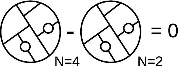
Let us begin at ${\cal O}(g^{2})$. The only diagram is a single gauge-field or scalar exchange. It is clear that the hypermultiplets play no rôle. Therefore the difference at this order in perturbation theory is identically zero. We can generalize this logic in the following way. Since the ‘‘source’’ fields, i.e. those coupled in the Wilson loop are common between the two theories, all diagrams which do not contain loops vanish identically in the difference³³ 3 This is because the couplings are at least quadratic in the hypermultiplet fields, see (26), (27)., see figure 1.

Now let us consider the diagrams at ${\cal O}(g^{4})$. There are three: the two-rung diagram, the trivalent graph consisting of a single cubic vertex with all three fields attached to the Wilson loop, and the one-loop-corrected one-rung diagram. By the logic just expounded upon, only the last diagram has a chance of surviving the difference. As we will now show, it too cancels-out. The colour factor in the one-loop correction to the gauge field $A_{\mu}$ (or real scalar $\Phi_{I}$) propagator stemming from a loop of one adjoint field, or $2N$ fundamental fields is the same

$$\begin{split}&\text{1 adjoint field}\to i^{2}f^{qik}f^{kjq}=N\delta^{ij}\\ &\text{$2N$ fundamental fields}\to 2N\mathop{\mathrm{Tr}}(T^{i}T^{j})=N\delta^{ij}.\end{split}$$

(14)

Thus we are also free to decorate the diagrams of figure 1 with one-loop-corrected propagators, see figure 2.

It is worth underscoring at this point that we have now found agreement with the matrix model results presented in section 2 at the first two consecutive orders of perturbation theory, without evaluating a single Feynman diagram. At the next order, ${\cal O}(g^{6})$, we will have to do more work. Applying the rules depicted in figures 1 and 2, the only diagrams remaining are bona fide two-loop matter⁴⁴ 4 By “matter” we mean the fields in the hypermultiplet, whether they are in the adjoint or fundamental representation. corrections to the gauge/scalar propagator and bona fide one-loop matter corrections to the triple vertex, see figure 3.

Let us concentrate on the former. We can reduce this class of diagram even further. Introducing a fat graph notation, where fundamental fields are represented by single lines, and adjoint ones by double lines, we find that the following topology of diagram cancels between the ${\cal N}=4$ and ${\cal N}=2$ theories

$\sim 2N\,if^{qik}\mathop{\mathrm{Tr}}(T^{k}T^{j}T^{q})=\frac{N^{2}}{2}\delta^{ij}$

It turns out that $\zeta(3)$ is very hard to come by in these Feynman diagrams. In fact, the only time it appears is from the well-known integral

$${\cal I}=\int\frac{d^{4}k}{(2\pi)^{4}}\int\frac{d^{4}q}{(2\pi)^{4}}\frac{1}{k^{2}q^{2}(k-p)^{2}(q-p)^{2}(k-q)^{2}}=\frac{1}{(4\pi)^{4}p^{2}}\,6\,\zeta(3),$$

(16)

arising solely from the topology:

which typically also contains other terms (owing to numerators), however these other terms do not contain $\zeta(3)$. The general structure of these diagrams is as follows

$$\frac{(p^{2})^{1-2\epsilon}}{(4\pi)^{4-2\epsilon}}\left[A_{1}\left(\frac{1}{\epsilon^{2}}-\zeta(2)\right)+\frac{A_{2}}{\epsilon}+A_{3}+A_{4}\,\zeta(3)+{\cal O}(\epsilon)\right],$$

(17)

where $p$ is the external momentum, and where the $A_{i}$ are rational numbers⁵⁵ 5 The Euler-gamma terms have been removed through the usual $e^{2\epsilon\gamma}$ factor.. This structure is also found for all the other two-loop matter correction diagrams, albeit with $A_{4}=0$. In summing the contributions from all diagrams we find that the coefficients $A_{1}$, $A_{2}$, and $A_{3}$ sum to zero, and so all divergences and non-$\zeta(3)$ terms cancel entirely. The details of the calculation are collected in appendix A.

The diagrams responsible for the $\zeta(3)$ terms are shown below, where the solid (dashed) lines in the loop indicate the scalar (fermion) fields of the hypermultiplet. The external lines represent the adjoint gauge field (wiggly) or real scalar field (straight)⁶⁶ 6 Note that for fermion loops the real scalar field is also exchanged in the loop. For convenience we have let the vertical wiggly line represent both gauge and scalar exchange in this instance.. Let us begin by calculating the colour factor associated with these diagrams. We are interested in the difference between taking the matter in the adjoint and $2N$ times in the fundamental, the result being

$$\begin{split}&i^{4}f^{qik}f^{klr}f^{rjm}f^{mlq}-2N\mathop{\mathrm{Tr}}[T^{i}T^{k}T^{j}T^{k}]=\frac{N^{2}}{2}\delta^{ij}-2N\frac{-\delta^{ij}}{4N}=\frac{N^{2}+1}{2}\delta^{ij}.\end{split}$$

(18)

Since in the perturbative expansion of the Wilson loop to second order, i.e. two fields emanating from the loop, one gains a factor of $\mathop{\mathrm{Tr}}(T^{i}T^{i})/N\sim(N^{2}-1)/N$, one can already verify that the correct colour factor has emerged for a match to (11). Explicitly we find that the colour-stripped diagram-differences yield the following results

	$\displaystyle\parbox{91.04881pt}{\begin{fmfgraph*}{3}0,20) \fmffixed{(0,43)}{v2,v4} \end{fmfgraph*}}-\parbox{91.04881pt}{\begin{fmfgraph*}{3}0,20) \fmffixed{(0,43)}{v2,v4} \end{fmfgraph*}}$	$\displaystyle=\frac{4}{3}\,p^{4}\,\left(\delta^{\mu\nu}-\frac{p^{\mu}p^{\nu}}{p^{2}}\right)\,{\cal I}+\text{non-$\zeta(3)$}$
	$\displaystyle\parbox{91.04881pt}{\begin{fmfgraph*}{3}0,20) \fmffixed{(0,43)}{v2,v4} \end{fmfgraph*}}-\parbox{91.04881pt}{\begin{fmfgraph*}{3}0,20) \fmffixed{(0,43)}{v2,v4} \end{fmfgraph*}}$	$\displaystyle=\frac{8}{3}\,p^{4}\,\left(\delta^{\mu\nu}-\frac{p^{\mu}p^{\nu}}{p^{2}}\right)\,{\cal I}+\text{non-$\zeta(3)$}$
	$\displaystyle\parbox{91.04881pt}{\begin{fmfgraph*}{3}0,20) \fmffixed{(0,43)}{v2,v4} \end{fmfgraph*}}-\parbox{91.04881pt}{\begin{fmfgraph*}{3}0,20) \fmffixed{(0,43)}{v2,v4} \end{fmfgraph*}}$	$\displaystyle=4\,p^{4}\,\delta^{IJ}\,{\cal I}+\text{non-$\zeta(3)$}$

where ${\cal I}$ is the expression given in (16), and the “non-$\zeta(3)$” terms are the divergences and constant terms shown schematically in (17), and which cancel identically against the rest of the diagrams, which have no $\zeta(3)$ contribution. It is clear that the gauge field and real scalar field propagator contributions are equal, as they are in the celebrated one-loop calculation for the ${\cal N}=4$ theory presented in [3]. Adding the external propagators to these amputated diagrams also reveals that the result is proportional to the bare propagators⁷⁷ 7 Up to the extra $p^{\mu}p^{\nu}/p^{2}$ factors, which may be removed by a gauge transformation. $\delta^{\mu\nu}/p^{2}$ and $\delta^{IJ}/p^{2}$, for the gauge, and real scalar fields respectively. Fourier transforming back to position space and evaluating the expectation value of the Wilson loop, one obtains (2). Plugging in the circular contour $x^{\mu}=(\cos\tau,\sin\tau,0,0)$, and $\Theta^{I}(\tau)=\delta^{I1}$, one obtains

$$\frac{|\dot{x}_{1}||\dot{x}_{2}|-\dot{x}_{1}\cdot\dot{x}_{2}}{4\pi^{2}(x_{1}-x_{2})^{2}}=\frac{1}{4\pi^{2}}\frac{1}{2}.$$

(19)

The result is that (2) is exactly the expression given in (11), namely

$$\frac{3\,\zeta(3)}{512\pi^{4}}\frac{(N^{2}-1)(N^{2}+1)}{N},$$

(20)

and so we have recovered the matrix model result from perturbation theory.

As stressed in the introduction, the difference between the Wilson loop in ${\cal N}=4$ and superconformal ${\cal N}=2$ SYM appears as a term proportional to the bare gauge field (and associated real scalar) propagator. This fact is independent of the shape of the Wilson loop, although we were primarily interested in the circle for obvious reasons. In this section we would like to point-out a couple of implications of this result.

We would like to thank Jan Plefka, Johannes Henn, and Filippo Passerini for discussions. This work is supported by the Volkswagen Foundation.

References

- [1] J. M. Maldacena, “Wilson loops in large N field theories,” Phys.Rev.Lett. 80 (1998) 4859–4862, arXiv:hep-th/9803002 [hep-th].
- [2] S.-J. Rey, S. Theisen, and J.-T. Yee, “Wilson-Polyakov loop at finite temperature in large N gauge theory and anti-de Sitter supergravity,” Nucl.Phys. B527 (1998) 171–186, arXiv:hep-th/9803135 [hep-th].
- [3] J. Erickson, G. Semenoff, and K. Zarembo, “Wilson loops in N=4 supersymmetric Yang-Mills theory,” Nucl.Phys. B582 (2000) 155–175, arXiv:hep-th/0003055 [hep-th].
- [4] N. Drukker and D. J. Gross, “An Exact prediction of N=4 SUSYM theory for string theory,” J.Math.Phys. 42 (2001) 2896–2914, arXiv:hep-th/0010274 [hep-th].
- [5] V. Pestun, “Localization of gauge theory on a four-sphere and supersymmetric Wilson loops,” arXiv:arXiv:0712.2824 [hep-th].
- [6] F. Passerini, “Gauge Theory Wilson Loops and Conformal Toda Field Theory,” JHEP 1003 (2010) 125, arXiv:arXiv:1003.1151 [hep-th].
- [7] N. Drukker, D. R. Morrison, and T. Okuda, “Loop operators and S-duality from curves on Riemann surfaces,” JHEP 0909 (2009) 031, arXiv:arXiv:0907.2593 [hep-th].
- [8] N. Drukker, J. Gomis, T. Okuda, and J. Teschner, “Gauge Theory Loop Operators and Liouville Theory,” JHEP 1002 (2010) 057, arXiv:arXiv:0909.1105 [hep-th].
- [9] N. Drukker, D. Gaiotto, and J. Gomis, “The Virtue of Defects in 4D Gauge Theories and 2D CFTs,” arXiv:arXiv:1003.1112 [hep-th]. * Temporary entry *.
- [10] L. F. Alday, D. Gaiotto, S. Gukov, Y. Tachikawa, and H. Verlinde, “Loop and surface operators in N=2 gauge theory and Liouville modular geometry,” JHEP 1001 (2010) 113, arXiv:arXiv:0909.0945 [hep-th].
- [11] K. Zarembo, “Supersymmetric Wilson loops,” Nucl.Phys. B643 (2002) 157–171, arXiv:hep-th/0205160 [hep-th].
- [12] N. Drukker, S. Giombi, R. Ricci, and D. Trancanelli, “Supersymmetric Wilson loops on S**3,” JHEP 0805 (2008) 017, arXiv:arXiv:0711.3226 [hep-th].
- [13] S.-J. Rey and T. Suyama, “Exact Results and Holography of Wilson Loops in N=2 Superconformal (Quiver) Gauge Theories,” arXiv:arXiv:1001.0016 [hep-th].
- [14] A. Agarwal and D. Young, “Supersymmetric Wilson Loops in Diverse Dimensions,” JHEP 0906 (2009) 063, arXiv:arXiv:0904.0455 [hep-th].
- [15] Z. Guralnik and B. Kulik, “Properties of chiral Wilson loops,” JHEP 0401 (2004) 065, arXiv:hep-th/0309118 [hep-th].
- [16] Z. Guralnik, S. Kovacs, and B. Kulik, “Less is more: Non-renormalization theorems from lower dimensional superspace,” Int.J.Mod.Phys. A20 (2005) 4546–4553, arXiv:hep-th/0409091 [hep-th].
- [17] N. Drukker, S. Giombi, R. Ricci, and D. Trancanelli, “More supersymmetric Wilson loops,” Phys.Rev. D76 (2007) 107703, arXiv:arXiv:0704.2237 [hep-th].
- [18] N. Drukker, S. Giombi, R. Ricci, and D. Trancanelli, “Wilson loops: From four-dimensional SYM to two-dimensional YM,” Phys.Rev. D77 (2008) 047901, arXiv:arXiv:0707.2699 [hep-th].
- [19] A. Bassetto, L. Griguolo, F. Pucci, and D. Seminara, “Supersymmetric Wilson loops at two loops,” JHEP 06 (2008) 083, arXiv:0804.3973 [hep-th].
- [20] D. Young, “BPS Wilson Loops on S**2 at Higher Loops,” JHEP 0805 (2008) 077, arXiv:arXiv:0804.4098 [hep-th].
- [21] A. Bassetto, L. Griguolo, F. Pucci, D. Seminara, S. Thambyahpillai, et al., “Correlators of supersymmetric Wilson-loops, protected operators and matrix models in N=4 SYM,” JHEP 0908 (2009) 061, arXiv:arXiv:0905.1943 [hep-th].
- [22] A. Bassetto, L. Griguolo, F. Pucci, D. Seminara, S. Thambyahpillai, et al., “Correlators of supersymmetric Wilson loops at weak and strong coupling,” JHEP 1003 (2010) 038, arXiv:arXiv:0912.5440 [hep-th].
- [23] S. Giombi, V. Pestun, and R. Ricci, “Notes on supersymmetric Wilson loops on a two-sphere,” arXiv:arXiv:0905.0665 [hep-th].
- [24] S. Giombi and V. Pestun, “Correlators of local operators and 1/8 BPS Wilson loops on S**2 from 2d YM and matrix models,” arXiv:arXiv:0906.1572 [hep-th].
- [25] V. Pestun, “Localization of the four-dimensional N=4 SYM to a two-sphere and 1/8 BPS Wilson loops,” arXiv:arXiv:0906.0638 [hep-th].
- [26] J. Drummond, J. Henn, G. Korchemsky, and E. Sokatchev, “On planar gluon amplitudes/Wilson loops duality,” Nucl.Phys. B795 (2008) 52–68, arXiv:arXiv:0709.2368 [hep-th].
- [27] E. Glover, V. V. Khoze, and C. Williams, “Component MHV amplitudes in N=2 SQCD and in N=4 SYM at one loop,” JHEP 0808 (2008) 033, arXiv:arXiv:0805.4190 [hep-th].
- [28] S. Lal and S. Raju, “The Next-to-Simplest Quantum Field Theories,” Phys. Rev. D81 (2010) 105002, arXiv:0910.0930 [hep-th].
- [29] A. Gadde, E. Pomoni, and L. Rastelli, “Spin Chains in N=2 Superconformal Theories: From the Quiver to Superconformal QCD,” arXiv:arXiv:1006.0015 [hep-th].
- [30] A. Gadde, E. Pomoni, and L. Rastelli, “The Veneziano Limit of N = 2 Superconformal QCD: Towards the String Dual of N = 2 SU(N(c)) SYM with N(f) = 2 N(c),” arXiv:arXiv:0912.4918 [hep-th].
- [31] A. Grozin, “Lectures on QED and QCD,” arXiv:hep-ph/0508242 [hep-ph].