Collective dynamics in optomechanical arrays

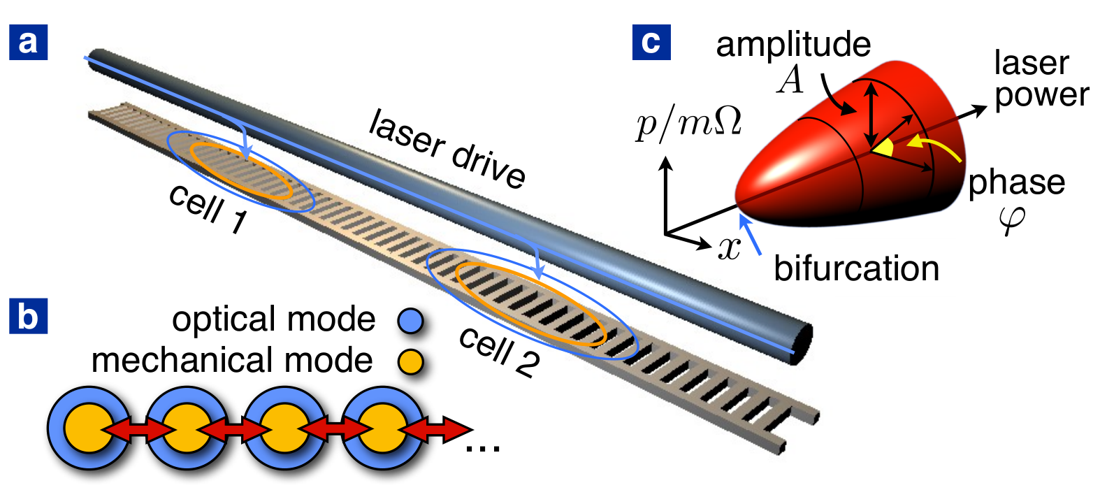
The emerging field of optomechanics seeks to explore the interaction between nanomechanics and light (see [1] for a recent review). Rapid progress in laser cooling of nanomechanical oscillators [2, 3] promises new fundamental tests of quantum mechanics [4], while applications benefit from ultrasensitive detection of displacements, masses and forces [5, 6, 7]. Recently, the exciting concept of optomechanical crystals has been introduced [8, 9, 10], where defects in photonic crystal structures are used to generate both localized optical and mechanical modes that interact with each other. For instance, this opens the prospect of integrated optomechanical circuits combining several functions on a single chip (see also [11, 12]). Here we start exploring the collective dynamics of arrays consisting of many coupled optomechanical cells (Fig. 1a,b). We show that such “optomechanical arrays” can display synchronization and that they can be described by a modified Kuramoto model that allows to explain and predict most of the features that will be observable in future experiments.

The crucial ingredient of any optomechanical system is an optical mode (OM) whose frequency shifts in response to a mechanical displacement: $\delta\omega_{{\rm opt}}=-Gx$. This coupling, vice versa, gives rise to a radiation force, $F=\hbar G|\alpha|^{2}$, where $|\alpha|^{2}$ is the number of photons circulating inside the laser-driven OM. For a laser red-detuned from the OM ($\Delta=\omega_{{\rm Laser}}-\omega_{{\rm opt}}<0)$, dynamical back-action effects induced by the finite photon decay time $\kappa^{-1}$ lead to cooling of the mechanical motion. In contrast, for blue detuning ($\Delta>0$), anti-damping results. Once this overcomes the internal mechanical friction, a Hopf bifurcation towards a regime of self-induced mechanical oscillations takes place (Fig. 1c) [14, 15, 16, 17, 13, 18]. While the mechanical amplitude $A$ is fixed, the oscillation phase $\varphi$ is undetermined. Therefore, it is susceptible to external perturbations. In particular, as we will see, it may lock to external forces or to other optomechanical oscillators.

Synchronization has first been discovered by Huygens and is now recognized as an important feature of collective nonequilibrium behavior in fields ranging from physics over chemistry to biology and neuroscience [19], with applications in signal processing and stabilization of oscillations. A paradigmatic, widely studied model for synchronization was introduced by Kuramoto [20]. For two oscillators, his phase evolution equation reads $\dot{\varphi}_{1}=\Omega_{1}+K\sin(\varphi_{2}-\varphi_{1})$, and likewise $\dot{\varphi}_{2}$. One finds synchronization ($\dot{\varphi}_{1}=\dot{\varphi}_{2}$) if the coupling $K$ exceeds the threshold $K_{c}=|\Omega_{2}-\Omega_{1}|/2$, and the phase lag $\delta\varphi=\varphi_{2}-\varphi_{1}$ vanishes for large $K$ according to $\sin(\delta\varphi)=(\Omega_{2}-\Omega_{1})/2K$. For the globally coupled, mean-field type version of infinitely many oscillators, there is a phase transition towards synchronization beyond some threshold $K_{c}$ that depends on the frequency distribution [21]. In many examples the Kuramoto model is found as a generic, reduced description of the phase dynamics. Nevertheless, for any specific system, it remains to be seen whether this model (or possibly a structurally similar variant thereof) applies at all, and how the coupling $K$ is connected to microscopic parameters [22, 23, 24]. We now turn to this question in the case of optomechanical oscillators.

A single optomechanical cell consists of a mechanical mode (displacement $x$) coupled to a laser-driven OM (light amplitude $\alpha$):

Here $\Omega$ is the mechanical frequency, $\Gamma$ the intrinsic damping, $G$ the optomechanical frequency pull per displacement, and $\alpha_{{\rm max}}$ is the maximum light-field amplitude achieved at resonance (set by the laser drive).

Near the Hopf bifurcation (Fig. 1c), we can capture the essential dynamics by eliminating the light field [16] and switching to the phase- and amplitude-dynamics of the resulting Hopf oscillator:

Here $\bar{A}$ is the steady-state amplitude, and $\gamma$ is the rate at which perturbations will relax back to $\bar{A}$. Both depend on the microscopic optomechanical parameters, such as laser detuning and laser drive power, and both vanish at the bifurcation threshold (see methods section). Moreover, we have introduced an external force $F(t)$ (as added to Eq. (2))

We start our discussion by considering phase-locking to an external force $F(t)=F_{0}\sin(\omega_{F}t)$. To this end we time-average Eq. (3), keeping only the slow dynamics, under the assumption $\omega_{F}\approx\Omega$. This results in

where $\delta\varphi=\varphi(t)+\omega_{F}t$, $\delta\Omega=\Omega-\omega_{F}$, and $K_{F}=F_{0}/2m\Omega\bar{A}$. Eq. (5) is a special case of the Kuramoto equation. Direct numerical simulation confirms the good agreement between the microscopic optomechanical dynamics and the simplified descriptions via Eqs. (3,4) and (5). In Fig. 2 we show $\sin\delta\varphi(t)$ and its time-average $\left\langle\sin\delta\varphi(t)\right\rangle$, with the phase $\varphi$ being extracted from the complex amplitude of motion, $\beta\equiv x+i\dot{x}/\Omega$. Phase-locking sets in when $\delta\dot{\varphi}=0$ has a solution, i.e. for $|\delta\Omega|\leq K_{F}$, resulting in an “Arnold tongue” (see Fig. 2d).

We now turn to the dynamics of coupled cells, each of which is described by Eqs. (1, 2). To these equations, we add a mechanical coupling, set by a spring constant $k$: $m\ddot{x}_{1}=\ldots+k(x_{2}-x_{1})$. In the Hopf model, this yields a force $F_{1}=kA_{2}\cos(\varphi_{2})$ on the first oscillator (and vice versa). The case of optical coupling will be mentioned further below.

In order to arrive at the time-averaged dynamics for the phase difference, $\delta\varphi=\varphi_{2}-\varphi_{1}$, it is necessary to go further than before, keeping $A(t)=\bar{A}+\delta A(t)$ in the phase equation, and eliminating the amplitude dynamics to lowest order (see methods for the derivation; and [25, 26] for further examples where the amplitude dynamics is crucial). Then, we arrive at an effective Kuramoto-type model for coupled optomechanical Hopf oscillators:

In contrast to the standard Kuramoto model, $2\delta\varphi$ appears, which will lead to both in-phase and anti-phase synchronization. This corresponds to two distinct minima in the effective potential that can be used to rewrite Eq. (6): $\delta\dot{\varphi}=-U^{\prime}(\delta\varphi)$. The coupling $K=k^{2}/2m^{2}\Omega^{2}\gamma$ diverges near the bifurcation, where $\gamma\rightarrow 0$. In the following we focus on the case of nearly identical cells where the coupling $C$ can be neglected; $C/\delta\Omega=k/2m\Omega^{2}\ll 1$.

To test whether these features are observed in the full optomechanical system, we directly simulate the motion and increase the coupling $k$ for a fixed frequency difference $\delta\Omega=\Omega_{2}-\Omega_{1}$. The results are displayed in Fig. 3(a-c). Beyond a threshold $k_{c}$, the frequencies and the phases lock, indicated by a kink in $\left\langle\sin\delta\varphi\right\rangle$. As the coupling increases further, the phases are pulled towards each other even more, so $\left|\delta\varphi\right|$ decreases. Thus, coupled optomechanical systems do indeed exhibit synchronization. As predicted, there is both synchronization towards $\delta\varphi\rightarrow 0$ and $\delta\varphi\rightarrow\pi$.

The dependence of the threshold $k_{c}$ on the frequency difference $\delta\Omega$ is shown in Fig. 3d. The observed behavior $k_{c}\sim\sqrt{\delta\Omega}$ at small $\delta\Omega$ is correctly reproduced by the generalized Kuramoto model, Eq. (6). For $\delta\Omega>\gamma$ deviations occur via terms of higher order in $\delta\Omega/\gamma$, starting with $-(\delta\Omega/\gamma)K\cos(2\delta\varphi)$ in Eq. (6). These produce a linear slope $k_{c}\propto\delta\Omega$, see Fig. 3d.

In terms of experimental realization, optomechanical crystals [8, 9] offer a novel promising way to build arrays of optomechanical cells. They are fabricated as free-standing photonic crystal beams (Fig. 1a). Variations of the $\mu m$-scale lattice spacing produce both localized optical and vibrational modes. The strong confinement leads to extremely large optomechanical couplings, on the order of $G\sim 100\,{\rm GHz/nm}$. Typical parameters, that we use in our simulations for experimentally realistic results, are $G=\text{100 GHz/nm}$, mechanical frequency $\Omega=\text{1 GHz}$, mass $m=\text{100 fg}$, mechanical quality factor $Q_{M}=\Omega/\Gamma=100$, cavity decay rate $\kappa=\text{1 GHz}$ and laser input powers such that the circulating photon number $|\alpha_{\text{max}}|^{2}\gtrsim 100$.

To consider optomechanical arrays like in Fig. 1a, we use finite element methods (FEM) to simulate two identical cells arranged on the same beam (Fig. 4a,b). The optical and vibrational couplings mediated by the beam can be deduced from the splitting between the resulting symmetric/antisymmetric modes. The results shown in Fig. 4c,d validate the parameters considered above and indicate mechanical couplings $k/m\Omega^{2}\lesssim 0.01$. Due to the relatively strong optical coupling ($\sim\text{THz}$), distinct OMs in the individual cells can only be achieved by patterning them to have frequencies sufficiently different to prevent hybridization (Fig, 4e). This requires different laser colors to address each cell.

In experiments, a convenient observable would be the RF frequency spectrum of the light intensity emanating from the cells, $\left|\alpha\right|^{2}(\omega)$. We first show the spectrum as a function of frequency difference $\delta\Omega$ for two mechanically coupled cells, driven independently (Fig. 5a). Frequency locking is observed in an interval around $\delta\Omega=0$. Experimentally, the mechanical frequencies can be tuned via the “optical spring effect” [8].

The most easily tunable parameter is the laser drive power ($\propto\alpha_{{\rm max}}^{2}$). Synchronization sets in right at the Hopf bifurcation. For two cells (Fig. 5c), we recover the regimes of in-phase and anti-phase synchronization. They differ in the synchronization frequency, $\bar{\Omega}(\pi)-\bar{\Omega}(0)=k/m\Omega$. At higher drive, we find a transition towards de-synchronization. This remarkable behavior can be explained from our analytical results. We know that $\gamma$ increases away from the Hopf bifurcation (i.e. for higher drive), leading to a concomitant decrease in the effective Kuramoto coupling $K\propto 1/\gamma$, and finally a loss of synchronization. Near the transition, the frequencies fan out (as $\delta\Omega_{{\rm eff}}\propto\sqrt{\alpha_{{\rm max}}-\alpha_{c}}$). The multitude of peaks is produced due to nonlinear mixing. In some regimes, the Kuramoto model fails (Fig. 5d).

For large arrays, it will be most practical to have identical OMs that combine into extended ’molecular’ modes, one of which is then driven by a single laser via an evanescently coupled tapered fibre (Fig. 1a, Fig. 4e). For efficient excitation of self-induced oscillations, one has to ensure that the detuning $\Delta$ is equal to all the mechanical frequencies $\Omega_{j}$ in the array, to within $\left|\Delta-\Omega_{j}\right|<\kappa$. For arrays of reasonable size, the splittings between adjacent optical molecular modes will be more than $10^{2}$ times larger than $\kappa$, such that we can ignore all but one OM. This setup then leads to a global coupling of many nanoresonators to a single OM, such that

and the force on each resonator is given by $-\hbar G_{j}|\alpha|^{2}$. This setup comes close to realizing the all-to-all coupling most often investigated in the literature on the Kuramoto model.

For illustration, we chose $N=5$ cells (Fig. 5e). As before, we find synchronization regimes. In addition, at higher drive, a transition into chaos takes place. Analyzing the time-evolution in more detail, we observe transient fluctuations in amplitude and phase, with a strong sensitivity on changes in initial conditions (Fig. 5f). Note that in a single optomechanical cell one may also find chaotic behavior [14], but for far larger driving strengths.

Optomechanical arrays open up a new domain to study collective oscillator dynamics, with room-temperature operation in integrated nanofabricated circuits and with novel possibilities for readout and control, complementing existing research on Josephson arrays [22], laser arrays [23] and other nanomechanical structures [24, 27]. Recent experiments on 2D optomechanical crystals [28] could form the basis for investigating collective dynamics in 2D settings with various coupling schemes. Applications in signal processing may benefit from phase noise suppression via synchronization [29]. Variations of the optomechanical arrays investigated here may also be realized in other designs based on existing setups, like multiple membranes in an optical cavity [30] or arrays of toroidal microcavities [2, 5].

References

- [1] Marquardt, F. & Girvin, S. M. Optomechanics. Physics 2, 40 (2009).
- [2] Schliesser, A., Arcizet, O., Riviere, R., Anetsberger, G. & Kippenberg, T. J. Resolved-sideband cooling and position measurement of a micromechanical oscillator close to the Heisenberg uncertainty limit. Nat. Phys. 5, 509–514 (2009).
- [3] Gröblacher, S. et al. Demonstration of an ultracold micro-optomechanical oscillator in a cryogenic cavity. Nat. Phys. 5, 485–488 (2009).
- [4] Marshall, W., Simon, C., Penrose, R. & Bouwmeester, D. Towards quantum superpositions of a mirror. Phys. Rev. Lett. 91, 130401 (2003).
- [5] Anetsberger, G. et al. Near-field cavity optomechanics with nanomechanical oscillators. Nat. Phys. 5, 909–914 (2009).
- [6] Verlot, P., Tavernarakis, A., Briant, T., Cohadon, P.-F. & Heidmann, A. Scheme to probe optomechanical correlations between two optical beams down to the quantum level. Phys. Rev. Lett. 102, 103601 (2009).
- [7] Teufel, J. D., Donner, T., Castellanos-Beltran, M. A., Harlow, J. W. & Lehnert, K. W. Nanomechanical motion measured with an imprecision below that at the standard quantum limit. Nat. Nano. 4, 820–823 (2009).
- [8] Eichenfield, M., Camacho, R., Chan, J., Vahala, K. J. & Painter, O. A picogram- and nanometre-scale photonic-crystal optomechanical cavity. Nature 459, 550–555 (2009).
- [9] Eichenfield, M., Chan, J., Camacho, R. M., Vahala, K. J. & Painter, O. Optomechanical crystals. Nature 462, 78–82 (2009).
- [10] Chang, D., Safavi-Naeini, A. H., Hafezi, M. & Painter, O. Slowing and stopping light using an optomechanical crystal array. arXiv: eprint 1006.3829 (2010).
- [11] Li, M. et al. Harnessing optical forces in integrated photonic circuits. Nature 456, 480–484 (2008).
- [12] Li, M., Pernice, W. H. P. & Tang, H. X. Tunable bipolar optical interactions between guided lightwaves. Nat. Photon. 3, 464–468 (2009).
- [13] Höhberger, C. & Karrai, K. Self-oscillation of micromechanical resonators. Nanotechnology 2004, Proceedings of the 4th IEEE conference on nanotechnology 419 (2004).
- [14] Carmon, T., Rokhsari, H., Yang, L., Kippenberg, T. J. & Vahala, K. J. Temporal behavior of radiation-pressure-induced vibrations of an optical microcavity phonon mode. Phys. Rev. Lett. 94, 223902 (2005).
- [15] Kippenberg, T. J., Rokhsari, H., Carmon, T., Scherer, A. & Vahala, K. J. Analysis of radiation-pressure induced mechanical oscillation of an optical microcavity. Phys. Rev. Lett. 95, 033901 (2005).
- [16] Marquardt, F., Harris, J. G. E. & Girvin, S. M. Dynamical multistability induced by radiation pressure in high-finesse micromechanical optical cavities. Phys. Rev. Lett. 96, 103901 (2006).
- [17] Ludwig, M., Kubala, B. & Marquardt, F. The optomechanical instability in the quantum regime. New J. Phys. 10, 095013 (2008).
- [18] Metzger, C. et al. Self-induced oscillations in an optomechanical system driven by bolometric backaction. Phys. Rev. Lett. 101, 133903 (2008).
- [19] Pikovsky, A., Rosenblum, M. & Kurths, J. Synchronization: A Universal Concept in Nonlinear Sciences (Cambridge University Press, 2001).
- [20] Kuramoto, Y. Self-entrainment of a population of coupled nonlinear oscillators. In International Symposium on Mathematical Problems in Theoretical Physics, vol. 39, 420–422 (Springer, 1975).
- [21] Acebrón, J. A., Bonilla, L. L., Pérez Vicente, C. J., Ritort, F. & Spigler, R. The Kuramoto model: A simple paradigm for synchronization phenomena. Rev. Mod. Phys. 77, 137–185 (2005).
- [22] Wiesenfeld, K., Colet, P. & Strogatz, S. H. Synchronization transitions in a disordered Josephson series array. Phys. Rev. Lett. 76, 404–407 (1996).
- [23] Kozyreff, G., Vladimirov, A. G. & Mandel, P. Global coupling with time delay in an array of semiconductor lasers. Phys. Rev. Lett. 85, 3809–3812 (2000).
- [24] Cross, M. C., Zumdieck, A., Lifshitz, R. & Rogers, J. L. Synchronization by nonlinear frequency pulling. Phys. Rev. Lett. 93, 224101 (2004).
- [25] Aronson, D., Ermentrout, G. & Kopell, N. Amplitude response of coupled oscillators. Physica D 41, 403 – 449 (1990).
- [26] Matthews, P. C., Mirollo, R. E. & Strogatz, S. H. Dynamics of a large system of coupled nonlinear oscillators. Physica D 52, 293 – 331 (1991).
- [27] Zalalutdinov, M. et al. Frequency entrainment for micromechanical oscillator. Appl. Phys. Lett. 83, 3281–3283 (2003).
- [28] Safavi-Naeini, A. H., Mayer Alegre, T. P., Winger, M. & Painter, O. Optomechanics in an ultrahigh-Q slotted 2D photonic crystal cavity. arXiv: eprint 1006.3964 (2010).
- [29] Tallur, S., Sridaran, S., Bhave, S. A. & Carmon, T. Phase noise modeling of optomechanical oscillators arXiv: eprint 1006.3805 (2010).
- [30] Thompson, J. D. et al. Strong dispersive coupling of a high-finesse cavity to a micromechanical membrane. Nature 452, 72–75 (2008).