Investigating different structures for the $X(3872)$

Journal: Nuc. Phys. (Proc. Suppl.)

Stephan Narison Email: snarison@yahoo.fr Address: Laboratoire de Physique Théorique et Astroparticules, CNRS-IN2P3 & Université de Montpellier II,
Case 070, Place Eugène Bataillon, 34095 - Montpellier Cedex 05, France. Fernando S. Navarra Email: navarra@if.usp.br Address: Instituto de Física, Universidade de São Paulo, C.P. 66318, 05389-970 São Paulo, SP, Brazil Marina Nielsen Email: mnielsen@if.usp.br Corresponding author: Speaker Address: Instituto de Física, Universidade de São Paulo, C.P. 66318, 05389-970 São Paulo, SP, Brazil

Abstract

Using the QCD spectral sum rule approach we investigate different currents with $J^{PC}=1^{++}$ , which could be associated with the $X(3872)$ meson. Our results indicate that, with a four-quark or molecular structure, it is very difficult to explain the narrow width of the state unless the quarks have a special color configuration.

1 Introduction

In the last years, several new observations on hadron states came from a variety of facilities. These include, in particular, low-lying excitations of the charmonium states, like the $X(3872)$ [1], the $Y(4260)$ [2], the $Y(3940)$ [3] the $Z(3930)$ [4] the $X((3940)$ [5] and many others with higher masses. Among these new hadron states, some of them are good candidates for exotic structures like: hybrid mesons, four-quark states, cusp, glueball or meson-meson molecules [6]. In this work we use QCD spectral sum rules (QSSR/QCDSR) (the Borel/Laplace Sum Rules [7, 8, 9]) to study the two-point functions of the axial vector meson, $X(3872)$ , assumed to be a four-quark state. Experimental information about the $X(3872)$ and previous uses of the QCDSR to study the $X(3872)$ meson can be found in [10].

The idea of mesons as four-quark states is not new. Indeed, even Gell-Mann in his first work about quarks had mentioned that mesons could be made out of $(q\bar{q}),~(qq\bar{q}\bar{q})$ , … [11]. The well known example of applying the idea of four-quark states for mesons is for the light scalar mesons (the isoscalars $\sigma(500),~f_{0}(980)$ , the isodublet $\kappa(800)$ and the isovector $a_{0}(980)$ ) [12, 13]. In the four-quark scenario, mesons can be considered as states of diquark-antidiquark pairs, or molecular (two-meson) bound states. The idea of diquarks is almost as old as QCD [14] and have been the subject of intense study by many theorists [15]. As pointed out in [16], diquarks can form bound states, which can be used as degrees of freedom in parallel with quarks themselves. For a diquark-antidiquark state, the color singlet can be obtained with the diquark-antidiquark pairs in a $\bar{3}-3$ or $6-\bar{6}$ color configuration. In previous calculations some of us have considered the $X(3872)$ as being a tetraquark state in the $\bar{3}-3$ color configuration [17] and in a molecular $D^{*}D$ configuration [18]. The currents used in these studies were

	$\displaystyle j_{\mu}^{(3)}$	$\displaystyle=$	$\displaystyle{i\epsilon_{abc}\epsilon_{dec}\over\sqrt{2}}[(q_{a}^{T}C\gamma_{5}c_{b})(\bar{q}_{d}\gamma_{\mu}C\bar{c}_{e}^{T})$		(1)
		$\displaystyle+$	$\displaystyle(q_{a}^{T}C\gamma_{\mu}c_{b})(\bar{q}_{d}\gamma_{5}C\bar{c}_{e}^{T})]\;,$		(1)

for the tetraquark state in the $\bar{3}-3$ color configuration and

	$\displaystyle j^{mol}_{\mu}(x)$	$\displaystyle=$	$\displaystyle{1\over\sqrt{2}}\Big[\left(\bar{q}_{a}(x)\gamma_{5}c_{a}(x)\bar{c}_{b}(x)\gamma_{\mu}q_{b}(x)\right)$		(2)
			$\displaystyle-\left(\bar{q}_{a}(x)\gamma_{\mu}c_{a}(x)\bar{c}_{b}(x)\gamma_{5}q_{b}(x)\right)\Big],$		(2)

for the molecular $D^{*}D$ configuration. In the above equations $a,~b,~c,~...$ are color indices, $C$ is the charge conjugation matrix and $q$ denotes a $u$ or $d$ quark.

The results obtained with these two currents are very similar and the deviations between the two QCDSR results in the allowed Borel window are smaller than 0.01% [10].

Another possible current with $J^{PC}=1^{++}$ and the diquark-antidiquark in the color sextet configuration is

	$\displaystyle j_{\mu}^{(6)}$	$\displaystyle=$	$\displaystyle{i\over\sqrt{2}}[(q_{a}^{T}C\gamma_{5}\lambda^{S}_{ab}c_{b})(\bar{q}_{d}\gamma_{\mu}C\lambda^{S}_{de}\bar{c}_{e}^{T})~+$		(3)
		$\displaystyle+$	$\displaystyle(q_{a}^{T}C\gamma_{\mu}\lambda^{S}_{ab}c_{b})(\bar{q}_{d}\gamma_{5}C\lambda^{S}_{de}\bar{c}_{e}^{T})]\;,$		(3)

where $\lambda^{S}$ stands for the six symmetric Gell-Mann matrices $\lambda^{S}=\left(\lambda_{0},~\lambda_{1},~\lambda_{3},~\lambda_{4},~\lambda_{6},~\lambda_{8}\right)$ .

In the QCDSR approach, the mass of the particle can be determined by considering the two-point correlation function

\Pi_{\mu\nu}(q)=i\int d^{4}x~e^{iq.x}\langle 0|T[j_{\mu}(x)j^{\dagger}_{\nu}(0)]|0\rangle.

(4)

In the phenomenological side, Eq. (4) can be written as

\Pi^{phen}_{\mu\nu}(q^{2})={\lambda^{2}\over m_{X}^{2}-q^{2}}\left(-g_{\mu\nu}+{q_{\mu}q_{\nu}\over m_{X}^{2}}\right)+\cdots\;,

(5)

for the $X$ meson represented by the currents in Eqs. (1), (2) and (3). In Eq. (5), the dots denote higher resonance contributions that will be parametrized, as usual, through the introduction of the continuum threshold parameter $t_{c}$ , and where we have introduced the meson-current coupling, $\lambda$ , through the parametrization $\langle 0|j_{\mu}^{q}|X(q)\rangle=\lambda\epsilon_{\mu}(q)$ .

In the OPE side, we work at leading order and consider condensates up to dimension six. We can write the correlation function in the OPE side in terms of a dispersion relation. Generically, we have

\Pi^{OPE}(q^{2})=\int_{4m_{c}^{2}}^{\infty}ds{\rho(s)\over s-q^{2}}\;,

(6)

where the spectral density is given by the imaginary part of the correlation function: $\rho(s)={1\over\pi}\mbox{Im}[\Pi^{OPE}(s)]$ .

After making an inverse-Laplace (or Borel) transform on both sides, and transferring the continuum contribution to the OPE side, the sum rule can be written as

\lambda^{2}e^{-(m_{X}^{(N)})^{2}\tau}=\int_{4m_{c}^{2}}^{t_{c}}ds~e^{-s\tau}~\rho^{(N)}(s)\;,

(7)

where $N=3,mol,6$ are related with the currents in Eqs. (1), (2) and (3) respectively, and the complete expressions for $\rho^{(3)}(s)$ , $\rho^{(mol)}(s)$ and $\rho^{(6)}(s)$ are given in refs. [17, 18, 19].

Using the QCDSR method, one usually estimates the hadron mass from the ratio

{\cal R}_{N}={\int_{4m_{c}^{2}}^{t_{c}}ds~e^{-s\tau}~s~\rho^{(N)}(s)\over\int_{4m_{c}^{2}}^{t_{c}}ds~e^{-s\tau}~\rho^{(N)}(s)}\sim(m_{X}^{(N)})^{2}\;.

(8)

However, in this work, instead of evaluating the meson mass through Eq. (8), we will consider the double ratios (DR) of the sum rules (DRSR) [19]

r_{6/3}=\sqrt{{\cal R}_{6}\over{\cal R}_{3}}\simeq{m_{X}^{(6)}\over m_{X}^{(3)}},

(9)

and

r_{mol/3}=\sqrt{{\cal R}_{mol}\over{\cal R}_{3}}\simeq{m_{X}^{(mol)}\over m_{X}^{(3)}},

(10)

This quantity has the advantage to be less sensitive to the perturbative radiative corrections and continuum contributions than the single ratio in Eq. (8). Therefore, we expect that our results obtained to leading order in $\alpha_{s}$ will be quite accurate.

2 QCDSR Results

Refer to caption — Figure 1: The double ratio $r_{6/3}$ (solid line) and $r_{mol/3}$ (dashed line) as a function of $\tau$ for $\sqrt{t_{c}}=4.15~\penalty\,\mbox{GeV}$ .

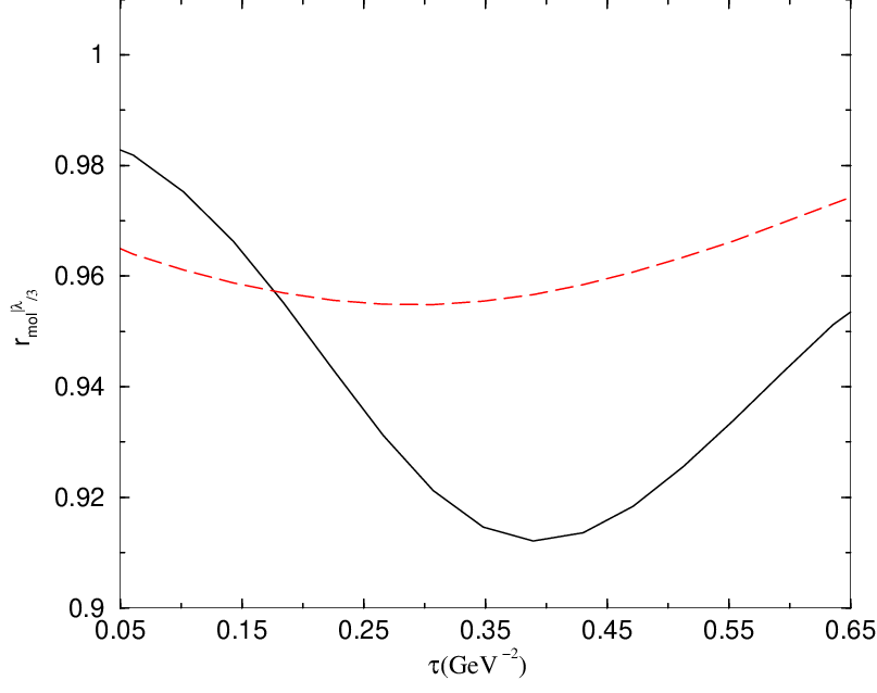
Fixing $\sqrt{t_{c}}=4.15~\penalty\,\mbox{GeV}$ , the value obtained in ref. [17], we show in Fig. 1 the $\tau$ -behaviour of $r_{6/3}$ (continuous line) and $r_{mol/3}$ (dashed line), using the QCD parameters presented in Table 1 [19].

Table 1: QCD input parameters.

Parameters	Values
$\Lambda(n_{f}=4)$	$(324\pm 15)$ MeV
$\hat{\mu}_{d}$	$(263\pm 7)$ MeV
$m_{0}^{2}$	$(0.8\pm 0.1)$ GeV²
$\langle\alpha_{s}G^{2}\rangle$	$(6\pm 1)\times 10^{-2}$ GeV⁴
$\rho\alpha_{s}\langle\bar{d}d\rangle^{2}$	$(4.5\pm 0.3)\times 10^{-4}$ GeV⁶
$m_{c}$	$(1.26\sim 1.47)$ GeV

From Fig. 1 one can notice that the results are very stable against the $\tau$ -variation in a large range for $\tau\leq 0.8$ GeV^-2 . We deduce

r_{6(mol)/3}=1.00,

(11)

with a negligible error, which shows that, from a QCD spectral sum rules approach, the $X(3872)$ can be equally described by the currents in Eqs. (1), (2) and (3).

The problem with these three currents is that a QCDSR study of the decay width of the decays $X\to J/\psi+3\pi$ and $X\to J/\psi+2\pi$ [19, 20], gives

\Gamma(X\to J/\psi+n\pi)|_{3,6,mol}\approx 50~{\rm MeV}~,

(12)

which is too big compared with the data upper limit [1]

\Gamma(X\to{\rm all})\leq 2.3~{\rm MeV}~.

(13)

The QCDSR study of the $X-\psi-V$ couplings, where the $2\pi$ and $3\pi$ can be assumed to come from the vector mesons $\rho$ and $\omega$ , is based on the three-point function

	$\displaystyle\Pi^{\mu\nu\alpha}(p,p^{\prime},q)$	$\displaystyle=$	$\displaystyle\int d^{4}x~d^{4}y~e^{i(p^{\prime}x+qy)}\times$		(14)
			$\displaystyle\langle 0\|{\cal T}J_{\psi}^{\mu}(x)J_{V}^{\nu}(y)J_{X}^{\alpha\dagger}(0)\|0\rangle$		(14)

associated to the $J/\psi$ -meson $J_{\psi}^{\mu}$ , vector mesons $J_{V}^{\nu}$ and to the $X$ -meson $J_{X}$ .

In the case of the three $X$ -currents ( $\bar{3}-3$ , $6-6$ tetraquarks and molecule) discussed above, the lowest order and lowest dimension contributing QCD diagrams are shown in Fig. 2.

As a matter of fact, a large partial decay width for the decay $X\to J/\psi V$ should be expected in this case. The initial state already contains all the four quarks needed for the decay, and there is no selection rules prohibiting the decay. Therefore, the decay is super-allowed through the fall-apart mechanism represented by the diagrams in Fig. 2. To avoid such fall-apart mechanism, the leading order contribution to the three-point function should be due to one gluon exchange, as shown in Fig. 3.

A possible current, for which the leading order contribution to the three-point function is due to one gluon exchange, as in Fig. 3, is the $\lambda$ -molecule $J/\psi-\pi$ -like current

j_{\mu}^{{mol}|^{\lambda}}=\left(\bar{c}\lambda^{a}\gamma_{\mu}c\right)\left(\bar{q}\lambda_{a}\gamma_{5}q\right)

(15)

where $\lambda_{a}$ is the colour matrix.

The corresponding spectral functions for this current are also given in Ref. [19]. In Fig. 4, we show the ratio of the $\lambda$ -molecule over the tetraquark $3-\bar{3}$ one.

In this case we get

r_{{mol|^{\lambda}}/3}=0.96\pm 0.03,

(16)

where the errors come from the stability regions and $m_{c}=1.26$ to 1.47 GeV (running MS and pole mass). This result suggests that the $X(3872)$ can have a large $\lambda$ -molecule component rather than a $6-6$ , $\bar{3}-3$ tetraquark or an (usual) $D-D^{(*)}$ molecule one. If this is the case, one expects, from Eq. (16), that the tetraquarks and $D-D^{(*)}$ molecule states are in the range of 3910-4160 MeV and with broader widths.

3 Conclusions

In conclusion, we have studied the mass of the $X(3872)$ using double ratios of sum rules. We found that the different proposed substructures ( $\bar{3}-3$ and $6-6$ tetraquarks and molecules) lead to the same mass predictions within the accuracy of the method [see Eq. (11)], indicating that the predictions of the $X$ meson mass is not sufficient for revealing its nature.

Among these different proposals, the only eventual possibility which can lead to a narrow width X(3872) is the choice of $\lambda$ -molecule- $J/\psi$ -like current given in Eq. (15). If this is the case, then the tetraquarks and $D-D^{(*)}$ molecule states are in the range of 3910-4160 MeV and with broader widths. Some further tests of this proposal are welcome.

Acknowledgements

M. Nielsen would like to thank the LPTA-Montpellier for the hospitality where this work has been initiated. This work has been partly supported by the CNRS-FAPESP within the QCD program, by CNPq-Brazil and by the IN2P3-CNRS within QCD program in Hadron Physics.

References

[1] Belle Coll., S.-L. Choi et al., Phys. Rev. Lett. 91, 262001 (2003).
[2] BABAR Coll., B. Aubert et al., Phys. Rev. Lett. 95, 142001 (2005).
[3] Belle Coll., S.-K. Choi et al., hep-ex/0505037, Phys. Rev. Lett. 94, 182002 (2005).
[4] Belle Coll., S. Uehara et al., Phys. Rev. Lett. 96, 082003 (2006).
[5] Belle Coll., K. Abe et al., hep-ex/0507019.
[6] for a review see E. S. Swanson, Phys. Rept. 429, 243 (2006).
[7] M.A. Shifman, A.I. and Vainshtein and V.I. Zakharov, Nucl. Phys. B147, 385 (1979).
[8] L.J. Reinders, H. Rubinstein and S. Yazaki, Phys. Rept. 127, 1 (1985).
[9] For a review and references to original works, see e.g., S. Narison, QCD as a theory of hadrons, Camb. Monogr. Part. Phys. Nucl. Phys. Cosmol. 17, 1-778 (2002) [hep-h/0205006]; QCD spectral sum rules , World Sci. Lect. Notes Phys. 26, 1-527 (1989); Acta Phys. Pol. B26 (1995) 687; Riv. Nuov. Cim. 10 (1987) 1; Phys. Rept. 84, 263 (1982).
[10] M. Nielsen, F.S. Navarra, S.H. Lee, arXiv:0911.1958.
[11] M. Gell-Mann, Phys. Lett. 8, 214 (1964).
[12] R.L. Jaffe, Phys. Rev. D15, 267, 281 (1977); D17, 1444 (1978).
[13] For a review see F.E. Close and N.A. Törnqvist, J. Phys. G28, R249 (2002).
[14] M. Ida and R. Kobayashi, Prog. Theor. Phys. 36, 846 (1966).
[15] For a review see, e.g., R.L. Jaffe, Phys. Rept. 409, 1 (2005).
[16] F. Wilczek, hep-ph/0409168.
[17] R.D. Matheus, S. Narison, M. Nielsen, J.M. Richard, Phys. Rev. D75, 014005 (2007).
[18] R. D. Matheus, F. S. Navarra, M. Nielsen, C. M. Zanetti, Phys. Rev. D80, 056002 (2009).
[19] S. Narison, F.S. Navarra, M. Nielsen, arXiv:1006.4802,
[20] F. Navarra and M. Nielsen, Phys. Lett. B639,272 (2006).

Investigating different structures for the X⁡(3872)X(3872)