Spin Path Integrals, Berry phase, and the Quantum Phase Transition in the sub-Ohmic Spin-boson Model

A quantum critical point (QCP) separates thermodynamic phases of matter at zero temperature and occurs when the order vanishes continuously as the zero-temperature phase transition is approached from the ordered side^{29, 21}. Quantum criticality has attracted considerable attention in recent years. This is not only due to the fact that quantum critical fluctuations are important in a broad temperature range around a QCP but has largely been fueled by the realization that not all continuous zero-temperature phase transitions may be described in terms of an order-parameter functional in elevated dimension^{37, 32, 2, 31}. The clearest experimental indication for such unconventional quantum criticality has so far come from anti-ferromagnetic heavy fermion metals⁷. The magnetic energy scales in these systems are small enough to tune the system from an itinerant anti-ferromagnet to a paramagnetic metal as an external tuning parameter is varied. In the traditional approach to the QCP in itinerant anti-ferromagnets, universal properties are described in terms of a Ginzburg-Landau-Wilson functional of the order parameter and its fluctuations resulting in a $\phi^{4}$-theory in $D+z$ dimensions, where $z=2$ is the dynamical exponent and $D$ is the spatial dimension of the system^{10, 22}. In contrast, a number of compounds which can be tuned through a zero-temperature transition do not follow the predictions of such a spin-density wave (SDW) theory^{1, 30, 25, 6}. This has led to the understanding that the concomitant destruction of the Kondo screening of the f-moments may result in an altered critical fluctuation spectrum^{2, 32}. One scenario, characterized by critical Kondo screening at the zero-temperature phase transition that is able to explain the experimental findings that are at variance with the conventional SDW picture has been termed ’local quantum criticality’^{32, 33}. A microscopic approach to the problem which preserves the dynamic competition between Kondo screening and magnetic correlations and consequently can capture the critical Kondo destruction is given by the Extended Dynamical Mean Field Theory (EDMFT)^{32, 34}. Within EDMFT, the Kondo lattice is mapped onto a quantum impurity model where a local moment is coupled to a fermionic and a bosonic bath and augmented with self-consistency requirements³³. This quantum impurity model is called the Bose-Fermi Kondo model (BFKM). The BFKM is, however, not only of interest in the context of the EDMFT approach to quantum critical heavy fermion compounds. The BFKM is also the effective low-energy model of single-electron transistors with ferromagnetic leads^{18, 15} and of Coulomb-blockaded noisy quantum dots¹¹. An interesting and important question is, under which conditions the QCP in the BFKM may be unconventional. After all, the EDMFT approach to the Kondo lattice preserves the dynamic competition between the local Kondo screening at each f-moment site and the magnetic fluctuations among different f-moments.
So far, this question has been addressed in the spin-isotropic and the easy-axis BFKM and the spin-boson model^{42, 8, 17, 39, 41, 40}. Based on a dynamical large-N limit, it was shown that the QCP in the spin-isotropic BFKM is in general not described in terms of a local $\phi^{4}$-theory⁴². This is in contrast to the critical behavior of a classical spin chain in $0+1$ dimension with a long-ranged interaction that is compatible with the retarded spin-spin interaction of the BFKM generated by the coupling to the fermionic and bosonic degrees of freedom^{4, 36}. As it turns out, the difference between the critical properties of the spin-isotropic BFKM and the classical spin chain is not spoiled by 1/N-corrections but can be traced back to the presence of a Berry phase term in the spin path integral representation of the quantum problem^{16, 14}. The quantum-to-classical mapping of quantum criticality that links a quantum-critical system to a $D+z$-dimensional classical critical system, therefore does not hold for the spin-isotropic BFKM ¹⁴.
The situation is at present less clear for the (spin-anisotropic) easy-axis BFKM and the spin-boson problem. While the two models are expected to belong to the same universality class, it is not clear whether the critical theory of the two models is identical to those of a local $\phi^{4}$-theory^{17, 41}. Numerical Renormalization Group (NRG) calculations point to a critical theory that is different from a local $\phi^{4}$-theory ^{39, 8, 9, 17}. The validity of such NRG calculations for critical systems involving bosons has however been called into question ^{41, 40, 38}. A recent continuous time Monte Carlo study ⁴¹ addresses the dissipative spin-boson model based on a Monte Carlo algorithm that explicitly takes the limit of vanishing lattice constant of a one-dimensional classical Ising chain ²⁸. In reference ¹⁷, it was pointed out that the continuum limit of the classical Monte Carlo misses the effects associated with properly regularizing the spin-flip terms. These topological excitations can be viewed as the analogue in the Ising case of the Berry phase effect in the spin-symmetric problem. This raises the question of the proper path integral of the spin-boson model and related Ising-anisotropic models in the continuum limit.
In what follows, I point out the role of the Berry phase in the path integral representation of the spin-boson model.

The sub-Ohmic spin-boson model is defined by

where $\sigma^{x}$ and $\sigma^{z}$ are generators of the su(2) algebra and $a_{q}$ and $a^{\dagger}_{q}$ follow bosonic commutation relations. For a sub-Ohmic spectral density of the bosons,

with $0<\eta<1$, the system undergoes a continuous quantum phase transition at a critical coupling $g_{c}$ that separates a localized from a delocalized phase. It is well established that the associated critical exponents obey hyperscaling for $\eta<1/2$. The situation for $1/2<\eta<1$ is less clear and has been discussed controversially ^{9, 17, 39, 41, 40}. This is so, because no reliable numerical method exists that allows to address Eq. (1) directly, despite the apparent simplicity of the spin-1/2 spin-boson model. The NRG method e.g. relies on a truncation of the bosonic Hilbert space. The starting point of a recent Monte Carlo study is an effective action description for the spin degrees of freedom. This relies on a particular functional integral representation of the spin-boson partition function and the applicability of an integral transformation

for Gaussian integrals within the path integral representation in order to integrate out the bosons ⁴¹.
A central question is, whether the effective action that results from integrating out the bosonic and fermionic degrees of freedom does assume the form of an order parameter or Ginzburg-Landau-Wilson (GLW) functional. Such a GLW functional then serves as the starting point for a proper RG analysis. For the spin-boson problem, the expectation value of the local spin operator $\sigma^{z}$ can be used as an order parameter. Ignoring any subtleties that arise when integrating out the bosons, one may conclude that the effective action is of the form

where $\phi_{n}$ is the Fourier component of the order parameter at the $n$th Matsubara frequency $\omega_{n}$. The term $|\omega_{n}|^{1-\eta}$ arises from a retarded long-ranged interaction $\sim|\tau|^{\eta-2}$, while $r_{0}$ measures the distance from the critical point and the term $\beta|\omega_{n}|^{2}$ represents a short-range interaction. Assuming the validity of the quantum-to-classical mapping, this last term is identified with $\Gamma\sigma^{x}$. The action Eq. (4) is equivalent to a one-dimensional spin-chain with long-range interaction $\sim r^{\eta-2}$ and its critical properties are well studied ^{4, 36}. In particular, consider a RG rescaling that transforms $\omega_{n}^{\prime}=b\omega_{n}$. Keeping the $\alpha$ term fixed implies $\phi_{n}^{\prime}=b^{(\eta-1)/2}\phi_{n}$. Therefore, $\beta$ changes as $b^{-1-\eta}$ and $u$ scales as $b^{1-2\eta}$. This implies that for $\eta>1/2$, $u$ scales to zero and the RG flow is governed by the Gaussian fixed point. As a result, hyperscaling breaks down for $\eta>1/2$. This is demonstrated in Figure 1 for $\eta=0.65$, where one finds $\chi_{c}(T=0,\omega_{n})\sim|\omega_{n}|^{\eta-1}$ and $\chi_{c}(T,\omega_{n}=0)\sim T^{-1/2}$ following reference ¹⁷. The fact, that $\eta-1\neq-1/2$ is a manifestation of the breakdown of hyperscaling.

In the following, some of the difficulties associated with the derivation of an effective local action are discussed and the need for spin coherent states in order to obtain a well-defined continuum limit is pointed out. A basic introduction into spin coherent states is provided. The central result of this article is that the effective action of the spin-boson model does not assume a form similar to Eq. (4) due to the presence of a corresponding Berry phase term. The considerations above, based on Eq. (4), therefore do not readily apply to the spin-boson model. In fact, a Berry phase term has been shown to change the critical behavior for $\eta>1/2$ in closely related models ¹⁶.

Path integrals have become a versatile tool in all areas of physics soon after their introduction into quantum mechanics by Feynman in 1948. In semiclassical calculations e.g. one can bring to bear its relation with the action of classical mechanics. For a problem involving spin this relation is less obvious and functional integral methods for spin systems are far less popular. Nonetheless, a number of distinct functional integral representations for spin Hamiltonians can be found in the literature ^{27, 3, 12, 24, 35, 28, 20}. For the spin-boson problem and in particular for constructing its effective action in the reduced Hilbert space of spin states not all functional integral representations are equally well suited. Fahri and Gutmann e.g. derived a functional integral directly from the Hamiltonian based on an orthogonal, countable basis of the Hilbert space on which the Hamiltonian operates ³. The spectrum of Eq. (1) is continuous so that the Fahri-Gutmann representation does not apply to the sub-Ohmic spin-boson problem. Furthermore, since paths are constructed as continuous Markov chains in the orthogonal basis, the resulting measure is in general non-Gaussian for the bosonic modes and the integral transformation, Eq.(3) is therefore not readily applicable. It therefore is far from obvious if or how an effective action could be obtained from the Fahri-Gutmann functional integral. To ensure the applicability of Eq. (3), the bosonic operators appearing in the functional integral of the spin-boson model, Eq. (1), will be represented by bosonic coherent states that diagonalize the bosonic annihilation operator $a|\phi\rangle=\phi|\phi\rangle$; where $\phi$ is a complex number, $\phi\,\in\,\mathbb{C}$. It can be shown that the overlap between bosonic coherent states is

for properly normalized coherent states such that $\langle\tilde{\phi}|\tilde{\phi}\rangle=1$. The resolution of unity in the single mode Hilbert space ${\mathcal{H}}_{B}$ in terms of the $|\phi\rangle$ becomes

For brevity, we will in this section only consider the Hamiltonian

since the extension to the full sub-Ohmic spin-boson problem will not pose any additional difficulties. The Hilbert space of the spin part of Eq. (7), ${\mathcal{H}}_{S}$, is spanned by the eigenstates of $\sigma^{z}$: $|S,m\rangle,~m\varepsilon\{-S,-S+1,\ldots,S\}$. For a spin-1/2 system, $S=1/2$, the resolution of unity in ${\mathcal{H}}_{S}$ becomes

and the matrix elements of $\sigma^{x}$ follow from $\sigma^{x}|\uparrow\rangle=|\downarrow\rangle,~\sigma^{x}|\downarrow\rangle=|\uparrow\rangle$. A basis of the Hilbert space of $H_{SB}$, ${\mathcal{H}}_{B}\otimes{\mathcal{H}}_{S}$, is therefore given by $|\phi\sigma\rangle=|\phi\rangle|\sigma\rangle$, where $\phi$ is an arbitrary complex number and $\sigma$ is either $\uparrow$ or $\downarrow$. The partition function $\mathcal{Z}$ of $H_{SB}$ therefore can be written as

where $A$ is a constant and $\epsilon=\beta/M$. Since $\epsilon\ll 1$, each of the matrix elements $\langle\sigma_{i}\phi_{i}|e^{-\epsilon H}|\sigma_{i+1}\phi_{i+1}\rangle$ appearing in Eq. (9) can be further simplified:

The spin basis is orthonormal, $\langle\sigma_{i}|\sigma_{i+1}\rangle=\delta_{\sigma_{i},\sigma_{i+1}}$. Therefore, the matrix element can be rewritten as

where $|\overline{\sigma}_{i+1}\rangle=|\uparrow\rangle$ if $|\sigma_{i+1}\rangle=|\downarrow\rangle$ or $|\overline{\sigma}_{i+1}\rangle=|\downarrow\rangle$ if $|\sigma_{i+1}\rangle=|\uparrow\rangle$ and $\sigma^{z}_{i+1}=\pm 1$ depending on the spin state $|\sigma_{i+1}\rangle$. In the final form of the matrix element, Eq. (11), no operators appear on the right hand side. As a consequence of the orthonormal spin basis, Eq. (11) assumes the form of a matrix exponential:

where matrix ${\bm{P}}^{i,i+1}=\exp(-\epsilon\mathbf{K}^{i,i+1})$ is defined for later use and ${\bm{K}}^{i,i+1}$ is the matrix

Note, the Pauli matrices appearing in Eq. (2) do not carry a time label and the $i$- and $(i+1)$-dependence of $\mathbf{K}^{i,i+1}$ is entirely due to the imaginary time dependence of the $\phi$ variable characterizing the boson state that enters the prefactors of $\bm{1}$ and ${\bm{\sigma}}^{z}$ of Eq. (18). The change in spin state during the time interval from $i$ to $i+1$ is determined by choosing one of the four matrix elements in Eq. (2). The structure of the matrix is the same for each of the $M$ time intervals but the diagonal elements depend on the time label $i$ through the boson. Inserting Eq. (2) into Eq. (9), the continuum limit $\epsilon\rightarrow 0$ cannot easily be performed, since one deals with matrix exponentials of non-commuting matrices. As a consequence, this representation does not allow to globally integrate out the bosonic degrees of freedom in a straightforward manner. Simply ignoring the complications that arise from the non-commuting matrices and taking $\epsilon\rightarrow 0$ and applying Eq. (3) would lead to terms of the form ${\bm{\sigma}}^{z}{\bm{\sigma}}^{z}=\bm{1}$, since the Pauli matrices do not carry a time label. If the coupling to the bosonic degrees of freedom vanishes, $g=0$, the matrix $\bm{K}$ at different times commutes and the continuum limit can be performed.
An apparent alternative seems to be to rewrite the matrix elements of $\bm{P}$ in Eq. (12) as the exponential of some function $F(S_{i},S_{i+1})$ with $S_{i}=\pm 1$:

This leads to

Eq. (19) can be inserted in Eq. (9) for the partition function. As is clear from e.g. the terms coupling to $S_{i}S_{i+1}$, the continuum limit $\epsilon\rightarrow 0$ can again not easily be taken. In particular, the bosonic field couples to the nearest neighbor coupling term $S_{i}S_{i+1}$ through $c$ of Eq. (19), that otherwise would give rise to a short-range coupling as in Eq. (4). The difficulties encountered in the path integral representation above are related to the orthogonality of the spin basis in ${\mathcal{H}}_{S}$ while the basis in ${\mathcal{H}}_{B}$ has the property $\langle\phi|\phi^{\prime}\rangle\neq 0$. If the coupling to the bosons vanishes ($g=0$), Eq. (19) reduces to the standard transfer-matrix of a quantum spin in a transverse field $\Gamma$ and standard methods apply ¹⁹.
As noted above, a strategy of choosing orthonormal bases for both ${\mathcal{H}}_{S}$ and ${\mathcal{H}}_{B}$ is problematic because Eq. (3) would no longer be applicable. A more viable option lies in the construction of an overcomplete basis in ${\mathcal{H}}_{S}$ in close analogy to the bosonic coherent states. These states are therefore called spin coherent states.

Spin coherent states were first introduced by J. Radcliffe in 1971 ²⁷ and are discussed e.g. in ^{12, 26, 20, 5}. Let us start considering the spin-1/2 problem. The physical state of such a two-level system is specified by a state vector

up to a phase; the Hilbert space is spanned by the two basis states $|\downarrow\rangle,~|\uparrow\rangle$ with $\langle\uparrow|\downarrow\rangle=0$. Thus, the one-dimensional projector

with $\mbox{Tr}({\mathcal{P}}_{\Psi})=1$ completely specifies the state of the two-level system. Here, ${\bm{\sigma}}^{x},~{\bm{\sigma}}^{y},~{\bm{\sigma}}^{z}$ are the Pauli matrices and ${\bm{1}}$ is the $2\times 2$ unit matrix. It follows that $n_{x}^{2}+n_{y}^{2}+n_{z}^{2}=1$ and ${\mathcal{P}}_{\Psi}$ is mapped onto a point $P=(n_{x},n_{y},n_{z})$ on a sphere of radius $1$, while the orthogonal state vector ${\mathcal{Q}}_{\Psi}=1-{\mathcal{P}}_{\Psi}$ corresponds to the point $Q=(-n_{x},-n_{y},-n_{z})=-P$ of the Bloch sphere. Any point $P^{\prime}=(n_{x}^{\prime},n_{y}^{\prime},n_{z}^{\prime})$ on the sphere can be mapped onto any other point $P=(n_{x},n_{y},n_{z})$ via a similarity transform,

where ${\bm{V}}$ is a member of the group SU(2). The dynamics of the two-level system are described by paths on the Bloch sphere generated by the time evolution operator associated with a particular Hamiltonian. The spin part of such a Hamiltonian is an element of the su(2) algebra and generates a mapping into SU(2) via the exponential map. Apparently, ${\bm{V}}={\bm{1}}$ and ${\bm{V}}=-{\bm{1}}$ leave ${\mathcal{P}}_{\Psi}$ invariant. This is a manifestation of the adjoint representation of SU(2) on which the mapping onto the Bloch sphere builds.

In order to define spin-coherent states, it is useful to note that if the $|\downarrow\rangle$-state, corresponding to the south pole of the sphere, is chosen as a reference state, only the north pole has a vanishing overlap with the reference state. Any other point on the sphere will correspond to a state that has a non-vanishing overlap with $|\downarrow\rangle$. This suggests, to define a spin-coherent state $|z\rangle$ via^{27, 12}.

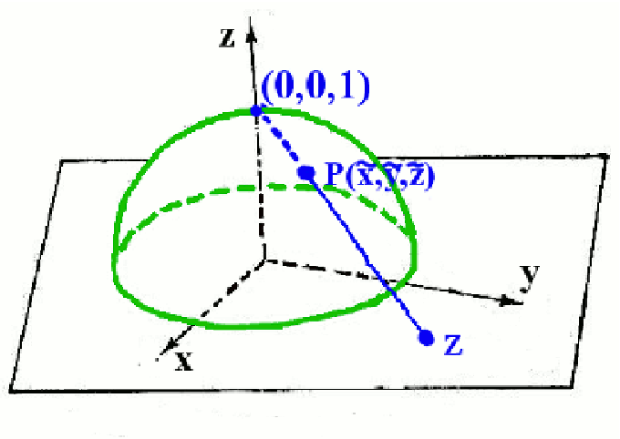
in close analogy to the definition of bosonic coherent states. where $z\in\mathbb{C}$ is a complex number and $c=(1+|z|^{2})^{-1/2}$ follows from $\langle z|z\rangle=1$ and $J^{+}|\uparrow\rangle=0$. Consequently, the state $|z\rangle=|x+iy\rangle$ is represented by a point $(x,y)$ in the complex plane as well as by its image $P=(n_{x},n_{y},n_{z})$ on the Bloch sphere (also called $S^{2}$). The relation between $z$ in the complex plane and $P$ on $S^{2}$ follows from Eq. (3) and Eq. (25) and is just the stereographic projection, see Figure 2:

In the remainder of this section, the formulae necessary to set up the spin path integral are valid for a general representation $S$ of SU(2).

Recall, that for any irreducible representation $|S,m\rangle$ of SU(2),

In accordance with Eq. (25), the definition of the spin coherent state for general $S$ is

where Eq.(27) was used. From the orthogonality of the spin states, the normalization factor $c$ follows as $c=(1+|z|^{2})^{-S}$ and the expansion coefficient of $|z\rangle$ in terms of the $|S,m\rangle$ becomes

The resolution of unity for spin coherent states is given by

The proof of this equation is analogous to the one for boson coherent states²³. Using Eq. (30) and with the help of

Eq. (32) is shown to be equivalent to Eq. (29). Alternatively, one can make use of Schur’s first lemma according to which an operator must be a constant if this operator commutes with every element of an irreducible representation of SU(2) ²³. Hence, this operator must be proportional to the unit operator. For general $S>1/2$, the pure state space is not the Bloch sphere $S^{2}$. Nonetheless, since $S^{2}$ is the coset space of $SU(2)$, it will turn out that the spin path integral can be either formulated in the complex plane, using Eq. (32), or on $S^{2}$. From Eq. (32) and the stereographic projection, the measure

can be interpreted as the area element of the unit sphere $S^{2}$. This measure is the invariant measure over SU(2).

As mentioned above, spin coherent states are overcomplete and the overlap between spin coherent states $|z_{1}\rangle$ and $|z_{2}\rangle$ is

this follows directly from Eq. (25). The matrix elements of the spin operators $J^{x}$, $J^{y}$, and $J^{z}$ in the spin coherent state representation can be calculated from Eq. (25):

For the diagonal part, one therefore obtains

where $\vec{n}=(n_{x},n_{y},n_{z})$ is the point $P$ on the unit sphere $S^{2}$ onto which $z$ is mapped by the stereographic projection. The definition of the spin coherent state for general spin representation $S$ suggests, that a close relation might exist with bosonic coherent states for the case, where the series in Eq.(30) does not truncate, e.g. for $S\rightarrow\infty$. This limit of large S for the quantum critical point of the sub-Ohmic Bose-Fermi Kondo and spin-Boson models has been explored in ^{14, 13}.

Note, we did not assume any particular symmetry property of a spin Hamiltonian. All the properties discussed in this section are consequences of the various basis states for the Hilbert space of a quantum spin and will be valid for any spin Hamiltonian, spin-isotropic or not.

This section contains the derivation of the functional integral representation of the sub-Ohmic spin-boson model in terms of bosonic and spin coherent states and a short discussion of the so-called Berry phase of the spin path integral. We start again with

The resolution of unity in terms of boson and spin coherent states in the respective sub-spaces are

and

respectively. A basis of the full Hilbert space is given by $|\phi z\rangle$ where $\phi$ and $z$ are complex numbers, $\phi,z\,\in\,\mathbb{C}$ . Repeating the steps above in the derivation of the partition function in terms of a path integral in imaginary time yields:

Inserting $(M-1)$ times the resolution of unity ${\bm{1}}_{\phi}\otimes{\bm{1}}_{\sigma}$ in the product space yields

where $\tilde{A}=\Big(\frac{2S+1}{4\pi^{2}i}\Big)^{M}$ and $\epsilon=\beta/M$, with $M\gg\beta$. Each of the matrix elements $\langle z_{i}\phi_{i}|e^{-\epsilon H}|z_{i+1}\phi_{i+1}\rangle$ can then be cast into

Note the difference between the short-time propagators in Eqn. (10) and (47). This is a consequence of the overcompleteness of the $|z\rangle$ basis versus the orthogonality of the $|\sigma\rangle$ basis. From Eqs. (36)-(38), the matrix elements of the spin operators between coherent states become

and together with Eq. (35), the short-time matrix element can be rewritten as

According to the rules of thumb of path integration, it is only necessary to keep terms of order $\epsilon$ in the short time matrix elements. If one considers paths that obey $z_{i+1}-z_{i}=O(\epsilon)$ one obtains

The overlap between spin coherent states for $z_{i+1}-z_{i}\equiv x=O(\epsilon)$ can be cast into²⁰

where the $\doteq$ implies equality up to order $z_{i+1}-z_{i}=x=O(\epsilon)$. This suggests, that the overlap $\langle z_{i}|z_{i+1}\rangle$ can be related to the image of $z_{i}$ on $S^{2}$, provided $z_{i}$ and $z_{i+1}$ are close enough to each other ($\epsilon\rightarrow 0$). The short-time matrix element together with the normalizing factor $\exp[-\phi^{*}\phi]$ for the bosonic coherent state becomes