Exploration of the phase diagram of 5D anisotropic SU(2) gauge theory

In our simulations we used the Kennedy-Pendleton heat bath algorithm for the updating of the gauge field [15]. A sketch of the phase diagram was produced from simulations on a lattice volume $V=8^{5}$. However the identification of the various phases was done using much larger volumes. The critical points in the ($\beta^{{}^{\prime}}$,$\beta$) plane correspond to the peak of the relevant (space-like or transverse-like) susceptibility. For the study of the order of the transitions between the phases of the model we used volumes up to $16^{5}$ with high statistics runs. For the errors the jack-knife method has been used.

In the following we present first the phase diagram of the theory with a short description of the various phases and continue with a more detailed study of the model for different values of the gauge couplings $\beta$ and $\beta^{{}^{\prime}}$.

The phase diagram that we present in Fig. 1 has been produced using a number of measurements ranging from $10^{4}$ to $10^{5}$ (after thermalization) on $V=8^{5}$ volumes. The phase diagram consists of three phases. For pure gauge theories analytical predictions regarding the value of the plaquette in the strong and weak coupling regime are useful for the characterization of the various phases. We know that for the isotropic SU(2) model defined in D dimensions the plaquette in the strong coupling limit ($\beta_{g}\ll 1$) is given by the relation

while in the weak coupling ($\beta_{g}\gg 1$) we have

where $\beta_{g}$ denotes the (unique) gauge coupling.
The five dimensional isotropic pure SU(2) model is known to undergo a first order phase transition at approximately $\beta_{g}\simeq 1.63$ from a strong coupling confining phase $\mathbb{S}$, where the plaquette behaves as $\frac{\beta_{g}}{4}$, to a Coulomb phase $\mathbb{C_{5}}$ where the plaquettes asymptotically behave as $1-\frac{3}{5\beta_{g}}$, bold line $C$ in the phase diagram [16, 17]. The phase diagram of the anisotropic SU(2) model, with couplings ($\beta$, $\beta^{{}^{\prime}}$), consists of the two aforementioned phases, strong confining phase $\mathbb{S}$ (for small values of $\beta$, $\beta^{{}^{\prime}}$) and Coulomb 5D phase $\mathbb{C_{5}}$ (for large values of $\beta$, $\beta^{{}^{\prime}}$), plus a new phase $\mathbb{W}$ for large $\beta$ and small values of $\beta^{{}^{\prime}}$ ¹¹ 1 The so called ”Layer” phase in the anisotropic 5d pure U(1) case [9].. The phase $\mathbb{W}$ is the continuation of the weak coupling phase of the four dimensional SU(2), for non zero $\beta^{{}^{\prime}}$. In this phase the transverse-like plaquette $P_{5}$ behaves like $\frac{\beta^{{}^{\prime}}}{4}$ and the space-like plaquette $P_{S}$ takes the values $1-\frac{3}{4\beta}$ indicating a four dimensional space time.
In the rest of this paper we will try to determine the nature of the transitions between the three possible phases of the model.

We begin with the passage from the strong coupling confining phase $\mathbb{S}$ to the ‘‘Layer’’ one ²² 2 For the case of the “Layer” phase we use the term loosely., denoted by $\mathbb{W}$, horizontal shadow thick line in the phase diagram. From the perspective of the transverse plaquette the transition goes unnoticed since both phases exhibit confinement along the transverse direction. Thus it comes as no surprise that $P_{5}$ remains fixed at the strong coupling limit value $\frac{\beta^{{}^{\prime}}}{4}$ throughout the transition. As described above the mean value of the space plaquette $P_{S}$ for $\beta^{{}^{\prime}}\neq 0$ has the same value with the plaquette for the 4d SU(2) in the same coupling $\beta$. The space plaquette retains its value for a wide range of $\beta^{{}^{\prime}}$ with no volume dependence. 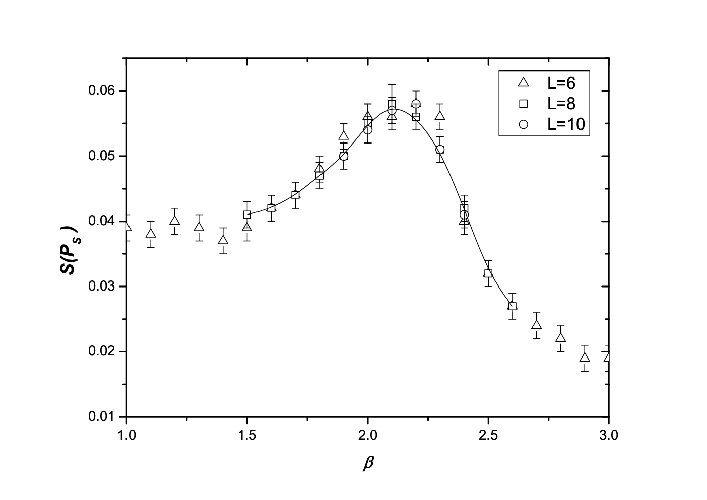In Fig. 2 we show the $\beta$-dependence of the susceptibility for the space plaquette at the point $\mathbb{A}$ in Fig. 1, corresponding to $\beta^{{}^{\prime}}=0.60$, for three different volumes (L=6,8 and 10). The peak of the space plaquette susceptibility $S(\hat{P}_{S})$ has the same value for the various volumes, so this transition is not really a phase transition. This line corresponds to a crossover from the strong coupling phase $\mathbb{S}$ to the weak coupling phase $\mathbb{W}$. Both regions describe the same physics with confinement at large distances and asymptotic freedom at small distances. The $\mathbb{W}$ region is a continuation of $\beta^{{}^{\prime}}=0$ behavior to $\beta^{{}^{\prime}}\neq 0$.

The next step involves the study of the Strong-Coulomb transition, $\mathbb{S}$ to $\mathbb{C_{5}}$, represented by the bold line $\mathbb{C}$ in the phase diagram of Fig. 1. Information on the transition is contained in both the space and transverse plaquettes. We study the transition along lines of constant $\beta$ and also along constant $\beta^{{}^{\prime}}$.
We present in Fig. 3(a) the histograms for the distribution $N(\hat{P}_{5})$ of the transverse plaquette $\hat{P}_{5}$ at the value $\beta=2.10$ which is located just below the Strong-Weak coupling phase boundary. As it is immediately apparent we are faced with a first order phase transition. In fact from the moment that we go from L=4 to L=6 the system, for the pseudo-critical value $\beta_{c}^{{}^{\prime}}$, spends its time in one or the other phase with no passages between the two. The same results are obtained for bigger values of $\beta^{{}^{\prime}}$ on the bold phase line $\mathbb{C}$ in Fig. 1, indicating a strong first order bulk phase transition which separates the phases $\mathbb{S}$, $\mathbb{C_{5}}$. As we move to bigger values of $\beta^{{}^{\prime}}$ on the phase line $\mathbb{C}$ the required volume to see signal for a first order bulk phase transition is increased [14, 18]. Note that the transition weakens as we move in the phase diagram to the left for smaller values of $\beta^{{}^{\prime}}$, bigger values of $\beta$.
In Fig. 3(b) we present the histogram for the transverse plaquette for the point $\mathbb{T}$, $\beta=2.50$, in the phase diagram. The lattice volume used is $16^{5}$ and $\beta^{{}^{\prime}}=0.8695$ on the maximum of transverse plaquette susceptibility, see Fig. 4(a). The two states in the histogram of Fig. 3(b) are barely distinguishable. As the transition weakens the two states come closer. This in turn results in a smaller barrier required by the system to overcome, in order to go from one state to the other, and consequently it does not spend a substantial amount of time in either one of them but rather goes back and forth between them for a small volume. Furthermore, the range of a distribution is proportional to the inverse of the square root of the volume of the system under study. For the particular volume the gap is of the same order of magnitude as the distributions range resulting in overlapping histograms for the two distinct phases.

For the point $\mathbb{T}$, $\beta=2.50$, we present also in Fig. 4 the transverse plaquette susceptibility $S(\hat{P}_{5})$ for various lattices $(L=10,12,14\textnormal{ and }16)$ as a function of $\beta^{{}^{\prime}}$ Fig. 4(a), and the maximum, $S_{max}$, of the transverse plaquette susceptibility versus $L$ in Fig. 4(b). For the smaller volumes under study (up to L=14) the system appears to undergo a continuous phase transition. The values of the plaquette change smoothly with $\beta^{{}^{\prime}}$ and the maximum of the susceptibility grows with a much smaller rate than one would expect from a first order transition. It is only at L=16 that the first indications of a first order transition appear. A faint two peak signal in the distribution of the transverse plaquette (Fig. 3(b)) accompanied by an abrupt change in the values of the susceptibility (Fig. 4). For a first order phase transition one expects the susceptibility to scale with the lattice volume. We observe indeed that the volume ratio is $(\frac{16}{14})^{5}\simeq 2$ and the obtained value for the transverse susceptibility gives $\frac{S_{max}(L=16)}{S_{max}(L=14)}\simeq 3$. We expect that this tendency for increasing the susceptibility in proportion to the lattice volume will persist for even bigger lattices. Compared to the smaller volumes under study the susceptibility for L=16 resembles more a delta function clear signal of a first order phase transition.

Define the transverse plaquette gap $G_{5}$ as the difference for the mean values for the transverse plaquette in the Coulomb phase $\mathbb{C_{5}}$ and the confining phase $\mathbb{S}$, $G_{5}=P_{5}(\mathbb{C_{5}})-P_{5}(\mathbb{S})$. We calculate the gap $G_{5}$ on the first order phase line $\mathbb{C}$ in the phase diagram (Fig. 1). The gap $G_{5}$ is presented in Fig. 5 versus $\beta$ for various lattice volumes. Each point in Fig. 5 represents a couple $(\beta^{{}^{\prime}},\beta)$ on this first order line. Various volumes were used in order to acquire a signal for a first order transition. For the cases where a clear two state signal is present in the distribution of the transverse plaquette the gap was calculated using independent Gaussian fits involving a close range of values around the two peaks. When a two peak signal could not be found we used extensive runs originating from the two different phases, with different initial values for the fields. As a result, for the same values of the parameters ($\beta^{{}^{\prime}}$,$\beta$), the system was found in one or the other phase depending on the initial conditions, providing us with an estimate for the gap. The behavior of the plaquette gap versus $\beta$ is quite interesting. It appears to increase in value until a plateau is reached in the region close to $\beta\simeq\beta^{{}^{\prime}}$. Afterwards, and as $\beta$ is increased further, its value is decreased rather rapidly, possibly reaching zero for values of $\beta\simeq 2.60$.

Of particular interest is the transition between the weak coupling phase $\mathbb{W}$ and the Coulomb (or deconfined) phase $\mathbb{C_{5}}$. It has been suggested in [12] that there is a line of second order phase transitions on the phase boundary. Our findings support the claim for a phase transition of second order or higher. We study in detail up to lattice volume $16^{5}$ two values of $\beta$. First point $\mathbb{B_{1}}$ with $\beta=3.00$ deep inside the weak coupling region of SU(2) and second, point $\mathbb{B_{2}}$ with $\beta=2.60$ near the expected, from our results, end of the first order phase transition.

For the first point $\mathbb{B_{1}}$ of the phase diagram, at $\beta=3.00$ the relevant observables are the transverse plaquette $P_{5}$ which should experience the passage from a confining behavior to a Coulomb one, and the transverse plaquette susceptibility $S(\hat{P}_{5})$. For our study we used six volumes (L=6, 8, 10, 12, 14 and 16) with the number of measurements ranging from $10^{5}$ to $2\times 10^{5}$ especially near the critical region. Our results for the transverse susceptibility $S(\hat{P}_{5})$ are summarized in Fig. 6. The plaquette $P_{5}$ itself has a weak volume dependence in the critical region and the plaquette distributions at the critical points lack a two peak signal, so a first order phase transition is excluded at least up to this lattice volume.
In the sequel we investigate if our results are compatible with a second order transition. For a second order phase transition we expect that near the critical point the correlation length is given by the relation

We assume that the pseudo-critical value of the transverse gauge coupling scales with the lattice length according to the expression [9]:

or equivalently:

The asymptotic scaling law for the susceptibility peak takes the form

The susceptibility $S(\hat{P}_{5})$ as a function of the five dimensional volume is depicted in Fig. 6. The susceptibility peaks display a weak scaling with the volume. The pseudocritical $\beta^{{}^{\prime}}_{c}$ and the maxima of the susceptibility, $S_{\textnormal{max}}(\hat{P}_{5})$, for each lattice volume have been estimated using the multihistogram method for all the points around the critical value and are given in Table 1.

Using Eq. (7) and Table 1 we obtain (Fig. 7(a)) the following values :

for the infinite volume value of $\beta^{{}^{\prime}}$ and the critical exponent $\nu$ with $\chi^{2}=1.27$.

An estimate for the other critical exponent $\gamma$ is given by :

In Ref.[12, 13], see also [18], the authors conclude that the second order phase transition may belong to the trivial 4d Ising universality class. Under this assumption we modify the relevant equations to include a logarithmic adjustment:

The above equation, which is valid for the 4D Ising model (Ref.[19, 20]), incorporates logarithmic corrections as opposed to the “naive” power-law behavior of Eq. (7). From Eq. (10) and Table 1 we have:

with $\chi^{2}=1.27$, no significant change in the quality of the fit is observed and the results are comparable with the previous values for $\nu$ and $\beta^{{}^{\prime}}$.
The scaling of the susceptibility is also modified accordingly:

Using the previous value of $\nu$ and Table 1 we have:

The values that we obtain are very far from those of the 4D Ising model ³³ 3 In the 4d Ising model $\nu=0.50$ and $\frac{\gamma}{\nu}=2.00$.. Both methods give a rough estimate $\frac{\gamma}{\nu}\sim 0.45$, indicating that the susceptibility scales with the lattice volume like a square root. If we do fix the value of $\frac{\gamma}{\nu}$ to the 4d Ising model value and repeat the fit for the maxima of the transverse susceptibility $S_{\textnormal{max}}(\hat{P}_{5})$, the result is bad with a big chi-square. We estimate that we need more statistics and bigger lattice volumes to be able to have a definite answer for the universality class of this phase transition.

Next we set the value of the space coupling to $\beta=2.60$ while we allow $\beta^{{}^{\prime}}$ to vary, point $\mathbb{B_{2}}$ in the phase diagram. We repeat the previous analysis for the new value of $\beta$ and the results are presented in Table 2.

From Table 2 and equations (7) and (9) we have:

with $\chi^{2}=0.25$ and $\chi^{2}=0.51$ respectively and the ratio $\frac{\gamma}{\nu}=2.54(53)$.
If we use Eqs. (10) and (11) we have for the critical exponents and the infinite volume limit of $\beta^{{}^{\prime}}$:

with $\chi^{2}=0.25$ and $\chi^{2}=0.52$ respectively and the ratio $\frac{\gamma}{\nu}=2.26(47)$. The above results are obtained after the exclusion of the point L=6 from the analysis. The ratio $\frac{\gamma}{\nu}$, from the two methods, is comparable within errors. We observe from our results that up to L=16 the scaling of the susceptibility gives no indication for the presence of a first order phase transition.

References

- [1] Th.Kaluza,Sitzungsber.d.Preuss.Akad.d.Wiss. (1921) 996; O.Klein,Zeitschrift f. Phys. (1926) 895.
- [2]
I. Antoniadis, Phys. Lett. (1990) 377;
Nima Arkani-Hamed, S.Dimopoulos, G.R.Dvali, Phys.Rev.:086004,1999;
Nima Arkani-Hamed, S.Dimopoulos, G.R.Dvali, Phys.Lett.:263-272,1998;
K.R. Dienes, E. Dudas and T. Gherghetta, Nucl. Phys. (1999), [hep-ph/9806292]. - [3]
L.Randall and R.Sundrum, Phys. Rev. Lett. 83 (1999) 4690, [hep-th/9906064];
Phys. Rev. Lett.83(1999)3370, [hep-ph/9905221]. - [4]
K. Farakos, P. Pasipoularides, Phys.Lett.:224-232,2005 [hep-th/0504014];
K. Farakos, P. Pasipoularides, Phys.Rev.:084012,2006 [hep-th/0602200];
K. Ohta and N. Sakai, Prog.Theor.Phys. 124 (2010) 71-93 [arXiv:1004.4078 [hep-th]];
Y. X. Liu, J. Yang, Z. H. Zhao, C. E. Fu and Y. S. Duan, Phys. Rev. D 80 (2009) 065019 [arXiv:0904.1785 [hep-th]];
Y. X. Liu, C. E. Fu, L. Zhao and Y. S. Duan, Phys. Rev. D 80 (2009) 065020 [arXiv:0907.0910 [hep-th]]. - [5]
Y.K. Fu and H.B. Nielsen, Nucl.Phys. , 167 (1984);
Y.K. Fu and H.B. Nielsen, Nucl.Phys. :127 (1985). - [6] K. Farakos, S. Vrentzos, Phys.Rev.:094511, (2008) [hep-lat/08013722].
- [7]
C.P. Korthals-Altes, S. Nicolis and J. Prades, Phys. Lett. 339 (1993) [hep-lat/9306017];
A. Hulsebos, C.P. Korthals-Altes and S. Nicolis, Nucl.Phys. 437 (1995) [hep-th/9406003]. - [8] P. Dimopoulos, K. Farakos, A. Kehagias, G. Koutsoumbas, Nucl.Phys. :237-252 (2001) [hep-th/0007079].
- [9] P. Dimopoulos, K. Farakos, S. Vrentzos, Phys.Rev.:094506 (2006) [hep-lat/0607033].
- [10]
P. Dimopoulos, K. Farakos, G. Koutsoumbas, Phys.Rev. :074505 (2001) [hep-lat/0111047];
P. Dimopoulos, K. Farakos, Phys.Rev. :045005 (2004) [hep-ph/0404288]. - [11] K. Farakos, S. Vrentzos, Phys.Rev.:114502 (2008) [hep-lat/08073463].
- [12]
N. Irges, F. Knechtli, Phys.Lett.:86-94,(2009) [hep-lat/09105427];
N. Irges, F. Knechtli, Nucl. Phys. B 822 (2009) 1 [arXiv:0905.2757 [hep-lat]]. - [13]
A. Kurkela, Ph. de Forcrand, M. Panero, Published in PoS LAT2009 (2009) 050 [arXiv:0911.3609 [hep-lat]];
Philippe de Forcrand, Aleksi Kurkela, Marco Panero, JHEP 1006 (2010) 050 [arXiv:1003.4643 [hep-lat]]. - [14] F.Knechtli, Magdalena Luz, Antonio Rago Nucl.Phys:7494 (2012) [hep-lat/1110420].
- [15] A. Kennedy and B. Pendleton, Phys. Lett. (1985) 393.
- [16] M. Creutz, Phys. Rev. Lett. (1979) 553.
- [17] K. Farakos, P. de Forcrand, C.P. Korthals Altes, M. Laine , M. Vettorazzo :170-184, (2003) [hep-ph/0207343].
- [18]
S.Ejiri, J.Kubo, M.Murata, Phys. Rev. :105025 (2000) [hep-ph/0006217];
S.Ejiri, S.Fujimoto, J.Kubo, Phys. Rev. :036002 (2002) [hep-lat/0204022]. - [19] E. Bittner, W. Janke, H. Markum, Phys.Rev.:024008, (2002) [hep-lat/0205023].
- [20] P.H. Lundow, K. Markström, Phys.Rev.:031104 (2009).